1 Introduction

The expansion of relativistic quantum field theory developed over 50 years ago by Feynman and Schwinger is still the basis for all perturbative calculations. However, analytical evaluations of graphs have become increasingly sophisticated, and digital computers make it possible to calculate graphs numerically. Since the accuracy of experiments in fundamental particle physics is continually improving, obtaining theoretical predictions whose precision matches that of the data requires the evaluation of ever larger numbers of more complex graphs. Moreover, non-Abelian and effective field theories also increase the variety of diagrams that must be considered. Thus the evaluation of Feynman diagrams remains an active area of research.

Many Feynman diagrams can be partially, or completely, evaluated with purely analytical methods. When a diagram cannot be reduced to a closed form, the remaining integrals must be tackled numerically. Since these integrals may be multi-dimensional, Monte Carlo integration is usually the only practical numerical algorithm [1, 2]. While conceptually simple, Monte Carlo methods converge slowly and accurate calculations of non-trivial graphs can be extremely time consuming. However, this combination of analytical and numerical techniques is extremely powerful and, for instance, makes it possible to evaluate all the eighth order graphs in QED which contribute to the electron magnetic moment [3]. In addition, computer algebra methods can be used to tackle the analytical categorization and simplification of diagrams, as summarized in the recent review [4].

In this paper, our immediate goal is to present a new approach to the numerical evaluation of Feynman diagrams. Its principal advantages are that it applies to arbitrary topologies, involves a minimal amount of analytic overhead, and has the potential to be much faster than Monte Carlo methods, especially when a result with more than one or two significant figures is required. The numerical method we develop is based on a novel representation of the Feynman integrals themselves, which allows us to approximate an arbitrary Feynman integral with a multi-dimensional infinite sum.

The basis of our approach is an approximation to the spacetime propagator, derived using the theory of generalized Sinc functions and expressed as an infinite sum. The approximation is governed by a small parameter, $h$, and converges rapidly to the exact result as $h\rightarrow 0$. For our purposes, the crucial feature of the approximate propagator is that its spatial (or momentum) dependence appears in terms like $\exp{(-(x-y)^{2})}$. When the propagators inside a Feynman integral are replaced with this approximate form, integrals over vertex locations or internal momenta required by the Feynman rules all reduce to Gaussian integrals, which can all be performed explicitly for any diagram. Once the Gaussian integrals have been performed, the result is an $N$-dimensional infinite sum, where $N$ is the number of propagators in the diagram. We refer to this infinite sum as the Sinc function representation of the Feynman integral.

An immediate advantage of the Sinc function representation is that sums are much easier to compute numerically than integrals, since sums are intrinsically discrete. More importantly, the general term in the sum decays exponentially, which greatly facilitates its numerical evaluation. We show that the effort needed to evaluate the $N$ dimensional Sinc function representation of a Feynman integral increases linearly with the desired number of significant figures, although for a complicated topology the constant of proportionality can be large. This is in contrast to Monte Carlo methods where each successive significant figure is generally more costly to obtain than the last, even when the convergence is improved through the use of adaptive sampling.

This paper introduces the Sinc function representation, and demonstrates its use in several explicit examples. We also present an approach to regularizing divergent diagrams and discuss the extraction of renormalization independent quantities in the context of the Sinc function representation. We focus our attention on scalar field theories in Euclidean spacetime, and will address the extension of Sinc function methods to more complicated theories in future work.

Finally, while the Sinc function representation applies to perturbative quantum field theory, the approximate propagator is also a key ingredient of a new approach to “exact” numerical quantum field theory, the ‘source Galerkin’ method [5, 6, 7, 8, 9]. The source Galerkin method also eschews the use of Monte Carlo calculations. In addition to improving its computational efficiency, by avoiding Monte Carlo techniques the source Galerkin method sidesteps many of the problems faced by other numerical approaches to non-perturbative quantum field theory, particularly in models with fermions. While the physical bases of the Sinc function representation and the source Galerkin method are very different, there is some intriguing evidence that insights gained while constructing the Sinc function representation may also allow us to improve the performance of the source Galerkin method.

The structure of this paper is as follows: In Section 2 we define the generalized sinc functions, and review their relevant properties. The Sinc function representation of the propagator is described in Section 3. In Section 4 we show this form of the propagator leads to a new representation for Feynman integrals, and derive the “Sinc function Feynman rules” for scalar field theory. We then apply these rules to the two loop “sunset” contribution to the $\lambda\phi^{4}$ two-point function, and compare our results to a conventional analytic calculation. In Section 5 we discuss techniques for efficiently evaluating the multi-dimensional sums obtained from the Sinc function Feynman rules. We then evaluate the sums derived for representative third and fourth order diagrams, and compare these calculations to direct integrations with VEGAS. Finally, in Section 6, we summarize our results and identify questions which we will pursue in future work.

2 Generalized Sinc Functions

We begin by describing a generalized Sinc function, which is defined by

$$S_{k}(h,x)=\frac{\sin{\left[\pi(x-kh)/h\right]}}{\pi(x-kh)/h}.$$ (1)

This is an obvious extension of the usual sinc function, $\mbox{sinc}(x)=\sin(x)/x$. Stenger [10] gives a thorough discussion of these functions, while a more introductory account is provided by Higgins [11]. We follow Stenger in using the capitalized “Sinc” to distinguish the generalized version, although our notation for $S_{k}(h,x)$ differs from his.

The Sinc function has the integral representation,

$$S_{k}(h,x)=\frac{h}{2\pi}\int_{-\pi/h}^{\pi/h}{e^{\pm i(x-kh)t}\,dt},$$ (2)

which is trivial to prove. We recognize equation (2) as the Fourier transform of a finite wavetrain, which is non-zero only in the interval $[-\pi/h,\pi/h]$. Using the integral representation, we can establish the orthonormality of the Sinc functions,

$$\int_{-\infty}^{\infty}{dx\,S_{k}(h,x)} = h,$$ (3)

$$\int_{-\infty}^{\infty}{dx\,S_{k}(h,x)S_{l}(h,x)} = h\delta_{kl}.$$ (4)

Any function $f(z)$, which is analytic on a rectangular strip of the complex plane, that is centered on the real axis with width $2d$, is approximated by

$$f(z)\approx\sum_{k=-\infty}^{\infty}f(kh)S_{k}(h,z).$$ (5)

The approximation improves as $h$ decreases, and this relationship is quantified below. Equation (5) is referred to as the “Sinc expansion” or “Sinc approximation” of $f(z)$. The Sinc expansion is exact for Paley-Weiner, or band-limited, functions, which corresponds to $f(z)$ be representable in the following way:

$$f(z)=\int_{-\pi/h}^{\pi/h}{g(u)e^{izu}\,du},\qquad g\in L^{2}(-\pi/h,\pi/h).$$ (6)

This states that $f$ is a function whose Fourier transform, $g$, has compact support on the interval $[-\pi/h,\pi/h]$ or, alternatively, that $f$ has no frequency outside the “band”, $[-\pi/h,\pi/h]$. Sinc functions are used in a wide variety of areas, and Stenger gives a number of examples from applied mathematics and classical physics. They are also at the basis of Shannon’s Sampling Theorem and are frequently encountered in communications theory.

For our purposes the most important property of the Sinc function is that if $f$ is approximated by its Sinc expansion, equation (5), we can quickly derive a related approximation for the definite integral,

$$\int_{-\infty}^{\infty}{f(z)\,dz} \approx \sum_{k=-\infty}^{\infty}\int_{-\infty}^{\infty}{dz\,f(kh)S_{k}(h,z)}$$ (7)

$$= h\sum_{k=-\infty}^{\infty}f(kh)$$

where the last equality follows from the normalization, equation (3). In the following section we use this relationship to approximate the propagator as an infinite sum.

From Theorem 3.1.2 of Stenger, the error in the Sinc approximation to a function $f(z)$ which is analytic in an infinite strip of the complex plane, centered upon the real axis with width $2d$, is

$$\delta f(h,z) = f(z)-\sum_{k=-\infty}^{\infty}f(kh)S_{k}(h,z)$$ (9)

$$= \frac{\sin{\frac{\pi z}{h}}}{2\pi i}\int_{-\infty}^{\infty}\left\{\frac{f(t-id)}{(t-z-id)\sin\left[\frac{\pi}{h}(t-id)\right]}\right.$$

$$\qquad+\left.\frac{f(t+id)}{(t-z+id)\sin\left[\frac{\pi}{h}(t+id)\right]}\right\}\,dt.$$

The discrepancy between $\int_{-\infty}^{\infty}f$ and its Sinc approximation is

$$\Delta f(h)=\int_{-\infty}^{\infty}{dz\,f(z)}-h\sum_{k=-\infty}^{\infty}f(kh).$$ (10)

Clearly, $\Delta f(h)$ is the result of integrating $\delta f(h,z)$ between $\pm\infty$, and Theorem (3.2.1) of Stenger allows us to deduce that

$$|\Delta f(h)|\leq C\frac{e^{-\pi d/h}}{2\sinh{\pi d/h}}$$ (11)

where $C$ is a real number which is independent of $h$. When $h<d$ we see that $|\Delta f(h)|$ drops exponentially as $h$ decreases linearly.

3 The Scalar Field Propagator

3.1 The Spacetime Propagator

Feynman diagrams are conventionally computed in momentum space, since the propagators are algebraically simpler, and the momentum conservation constraint at each vertex reduces the number of integrals that would otherwise need to be performed. However, we will find it more convenient to perform most of our work in coordinate space.

The spacetime propagator for a scalar field theory is the Fourier transform of the momentum space propagator,

$$G(p)=\frac{1}{p^{2}+m^{2}}$$ (12)

namely

$$G(x-y)=\int{\frac{d_{E}^{4}p}{(2\pi)^{4}}\frac{e^{ip(x-y)}}{p^{2}+m^{2}}},$$ (13)

where $x$, $y$ and $p$ are Lorentz four-vectors, and we are working in Euclidean space. Redefining $x-y$ as $x$ and adding a cut-off in anticipation of divergent diagrams, we can write

$$G_{\Lambda}(x)=\int{\frac{d_{E}^{4}p}{(2\pi)^{4}}\,\frac{e^{ipx}}{p^{2}+m^{2}}e^{-p^{2}/\Lambda^{2}}}.$$ (14)

Exponentiating the denominator gives

$$G_{\Lambda}(x)=\int{\frac{d_{E}^{4}p}{(2\pi)^{4}}\,e^{ipx-p^{2}/\Lambda^{2}}\int_{0}^{\infty}{dse^{-s(p^{2}+m^{2})}}}.$$ (15)

A rationale for this regulated form was given by Hahn [8]; in particular, formulating the cut-off in this way preserves the Gaussian form of the integrals (as would a dimensionally-regulated formulation). Reversing the order of integration, completing the square, performing the Gaussian integrals, and finally shifting from $s$ to $s/m^{2}$ yields

$$G_{\Lambda}(x)=\frac{m^{2}}{(4\pi)^{2}}\int_{0}^{\infty}{ds\,\frac{1}{(s+\frac{m^{2}}{\Lambda^{2}})^{2}}\exp{\left[-s-\frac{m^{2}x^{2}}{4(s+\frac{m^{2}}{\Lambda^{2}})}\right]}}.$$ (16)

Making a further change of variable to, $s=e^{z}$, we obtain

$$G_{\Lambda}(x) = \frac{m^{2}}{(4\pi)^{2}}\int_{-\infty}^{\infty}dz\,\frac{e^{z}}{(e^{z}+\frac{m^{2}}{\Lambda^{2}})^{2}}$$ (17)

$$\qquad\times\exp{\left[-e^{z}-\frac{m^{2}x^{2}}{4(e^{z}+\frac{m^{2}}{\Lambda^{2}})}\right]}.$$

The crucial step is to approximate $G_{\Lambda}(x)$ as an integral over a Sinc expansion [8] of the form given by equation (7),

$$G_{{\Lambda h}}(x) \approx \frac{m^{2}}{(4\pi)^{2}}\int_{-\infty}^{+\infty}dz\,\sum_{k=-\infty}^{\infty}{\frac{e^{kh}}{(e^{kh}+\frac{m^{2}}{\Lambda^{2}})^{2}}}$$ (18)

$$\qquad\times\exp{\left[-e^{kh}-\frac{m^{2}x^{2}}{4(e^{kh}+\frac{m^{2}}{\Lambda^{2}})}\right]}S_{k}(h,z)$$

$$= \frac{m^{2}h}{(4\pi)^{2}}\sum_{k=-\infty}^{\infty}\frac{e^{kh}}{(e^{kh}+\frac{m^{2}}{\Lambda^{2}})^{2}}$$

$$\qquad\times\exp{\left[-e^{kh}-\frac{m^{2}x^{2}}{4(e^{kh}+\frac{m^{2}}{\Lambda^{2}})}\right]}.$$

When $\Lambda\rightarrow\infty$ the coordinate space propagator, $G(x)$, can be expressed as a modified Bessel function of the second kind,

$$G(x)=\frac{m^{2}}{4\pi^{2}}\frac{K_{1}(m|x|)}{m|x|}.$$ (19)

In this limit, the Sinc approximation to $G_{\Lambda}$ also simplifies,

$$G_{{h}}(x)=\frac{m^{2}h}{(4\pi)^{2}}\sum_{k=-\infty}^{\infty}{\exp{\left[-kh-e^{kh}-\frac{m^{2}x^{2}}{4e^{kh}}\right]}}.$$ (20)

Finally, it will be convenient to introduce a more concise representation for the various factors that appear in the general term of sum,

$$G_{{\Lambda h}}(a-b)=\frac{m^{2}h}{(4\pi)^{2}}\sum_{k=-\infty}^{\infty}{p(k)\exp{\left[-\frac{m^{2}(a-b)^{2}}{4c(k)}\right]}}$$ (21)

where

$$c(k) = e^{kh}+\frac{m^{2}}{\Lambda^{2}},$$ (22)

$$p(k) = \frac{e^{kh}\exp{(-e^{kh})}}{(e^{kh}+\frac{m^{2}}{\Lambda^{2}})^{2}}=\frac{\exp{(kh-e^{kh})}}{c(k)^{2}}.$$ (23)

We now have four different versions of the propagator, which are related as follows. Firstly, the exact propagator, $G(x)$, is given by equation (19), while equation (16) defines the cut-off propagator, $G_{\Lambda}(x)$. These expressions are approximated by $G_{{h}}(x)$ and $G_{{\Lambda h}}(x)$ respectively, which are defined by equations (20) and (18). As we shall see, the approximations rapidly approach the exact values as $h$ becomes small.

Both the cut-off propagator, $G_{\Lambda}(a-b)$, and its approximation, $G_{{\Lambda h}}(a-b)$, depend only on the combination $(a-b)^{2}$, and thus neither the introduction of $\Lambda$ nor the Sinc function approximation has violated Poincaré invariance. Moreover, by Fourier transforming $G_{{\Lambda h}}(x)$ we could obtain a Sinc function approximation for the momentum-space propagator, equation (12), in the presence of the cut-off. In Section 4, we develop the Sinc function Feynman rules in coordinate space, but the momentum space rules could be obtained using an almost identical argument.

Figure 1: The relative error of the approximation $G_{{h}}$ is shown, by plotting $|\Delta G_{{h}}/G|$ as a function of $h$ for $m=x=1$ and $\Lambda\rightarrow\infty$.

Figure 2: The relative error of the approximation $G_{{h}}$ is shown, by plotting $|\Delta G_{{h}}/G|$ as a function of $x$ for $m=1$, $h=0.4$ and $\Lambda\rightarrow\infty$.

3.2 Accuracy of the Approximation

Our next task is to assess the accuracy of the approximation involved in writing $G_{{h}}(x)$ and $G_{{\Lambda h}}(x)$. We define

$$\Delta G_{{\Lambda h}}(x)=G_{\Lambda}(x)-G_{{\Lambda h}}(x).$$ (24)

The Sinc function approximation to the propagator is derived from equation (7), so the $h$ dependence of the error is governed by equation (11). The form of $f(z)$ which appears in the left hand side of equation (11) is our integrand,

$$f(z)=\frac{e^{z}}{(e^{z}+\frac{m^{2}}{\Lambda^{2}})^{2}}\exp{\left[-e^{z}-\frac{m^{2}x^{2}}{4(e^{z}+\frac{m^{2}}{\Lambda^{2}})}\right]}$$ (25)

where $x$, $m$ and $\Lambda$ are simply parameters. Since $f(z)$ is infinite when $e^{z}+m^{2}/\Lambda^{2}$ =0, or when $z=2\log(m/\Lambda)\pm i\pi$, it follows that $d$, the width of the strip of the complex plane which appears in equation (9), can take any value in the open interval $(0,\pi)$. Using the maximal possible value of $d$, we derive the following bound on the accuracy of the approximation,

$$|\Delta G_{{\Lambda h}}|\sim e^{-2\pi/h},\qquad h\rightarrow 0.$$ (26)

Thus as $h$ approaches zero, $\Delta f(h,z)$ decreases exponentially. Looking at the general form of the Sinc expansion, we see that the magnitude of the general term in the sum decreases (at least) exponentially with increasing $k$. Since any numerical evaluation of these sums must be cut off at finite $|k|$, it follows that while $G_{{\Lambda h}}$ will approach $G_{\Lambda}$ exponentially quickly as $h$ goes to zero, the number of terms that need be considered when computing the sum grows (at worst) linearly with $1/h$. This impressive convergence facilitates the numerical evaluation of the approximate propagators and, consequently, the Sinc function representations of the Feynman integrals.

Having discussed the abstract convergence properties of the Sinc approximation to the scalar field propagator, we now present some specific numerical results. Fig (1) shows $\Delta G_{{h}}(1)/G(1)$ as a function of $h$. These results were obtained using arbitrary precision arithmetic. When $h=0.1$, the two expressions differ by less than 1 part in $10^{-40}$, and if $h$ is even slightly less than unity the accuracy of the approximation is phenomenally impressive. As a specific example, choosing $h=0.5$ gives an accuracy of 1 part in $10^{8}$, while $h=0.25$ yields an agreement better than 1 part in $10^{16}$. On most computers, double precision real numbers contain 16 decimal digits, so if $h\lesssim 0.25$, $G_{{h}}(x)$ and $G(x)$ will be numerically indistinguishable. In fig. (2) we show that for fixed $h$, the accuracy of the approximation is essentially independent of $x$.

In figs (1) and (2) we have taken $\Lambda\rightarrow\infty$ for convenience, since this allows us to use the exact expression for the propagator, equation (19). However, using a finite value of $\Lambda$ makes no significant difference to these conclusions.

Figure 3: The number of significant terms in the series for $G_{{h}}(1)$, with $m=1$ is displayed. When the double infinite series for $G_{{h}}(x)$ is truncated at $k=-N$ and $k=N$, the result is accurate to within approximately 1 part in $10^{14}$. between

Our next concern is to determine how many terms in the series representation of $G_{{h}}$ contribute significantly to the final result when it is evaluated numerically. Fig (3) shows the number of terms in the series for $G_{{h}}$ which contribute more than 1 part in $10^{14}$ of the final result. If $h=0.25$, we need to include terms for which $|k|<21$. Note that this measures the convergence to $G_{{h}}$ rather than $G$, but for $h\lesssim 0.25$ the difference is less than the truncation error in the numerical calculation of $G_{{h}}(x)$. Also, if we do not need a highly accurate calculation, we can increase the value of $h$ and thus reduce the number of terms that contribute to the sum.

4 Evaluating Feynman Diagrams

4.1 The Sinc Function Representation

Having developed the Sinc function approximation to the propagator, we now turn to the evaluation of Feynman diagrams. In coordinate space the Feynman rules specify that we construct the product of the propagators corresponding to the $N$ internal lines of the diagram, and then integrate over each of the $M$ internal vertices. If the external lines are attached at the points $x_{1},x_{2},\cdots,x_{A}$ and the internal vertices are labeled by $y_{1},y_{2},\cdots,y_{M}$ we are therefore integrating over all spacetime for each of the $y_{j}$. Up to overall prefactors consisting of powers of the coupling constants and the topological weight of the diagram, these integrals take the form

$$I_{\Lambda} = \int d^{4}y_{1}\cdots d^{4}y_{M}G_{\Lambda}(x_{1}-y_{1})\cdots$$ (27)

$$\quad G_{\Lambda}(x_{A}-y_{j})\cdots G_{\Lambda}(y_{k}-y_{M}).$$

In general, the $I_{\Lambda}$ cannot be reduced to a closed, analytic form. We now use the Sinc expanded propagator, $G_{{\Lambda h}}$, to derive the Sinc function representation, $I_{{\Lambda h}}$, of a Feynman integral, $I_{\Lambda}$.

Firstly, $G_{\Lambda}(x)=G_{{\Lambda h}}(x)+\Delta G_{{\Lambda h}}(x)$. For given $\Lambda$ and $h$, there exists a number $c$, such that $\Delta G_{{\Lambda h}}(x)\lesssim cG_{\Lambda}(x)$, and $c\ll 1$ if $h$ is sufficiently small. We therefore obtain

$$I_{\Lambda} = \int d^{4}y_{1}\cdots d^{4}y_{M}\left[\right.(G_{{\Lambda h}}(x_{1}-y_{1})+$$ (29)

$$\qquad\Delta G_{{\Lambda h}}(x_{1}-y_{1}))\cdots$$

$$\quad\left.(G_{{\Lambda h}}(y_{k}-y_{M})+\Delta G_{{\Lambda h}}(y_{k}-y_{M}))\right]$$

$$\approx \int d^{4}y_{1}\cdots d^{4}y_{M}G_{{\Lambda h}}(x_{1}-y_{1})\cdots G_{{\Lambda h}}(y_{k}-y_{M})$$

$$\qquad{}+M\int d^{4}y_{1}\cdots d^{4}y_{M}\left[\Delta G_{{\Lambda h}}(x_{1}-y_{1})\cdots\right.$$

$$\qquad\left.G_{{\Lambda h}}(y_{k}-y_{M})\right],$$

where we have assumed that $h$ is small enough to make $\Delta G_{{\Lambda h}}(x)\ll G_{{\Lambda h}}(x)$, so we can drop terms that are second order in the $\Delta G_{{\Lambda h}}(x)$. Consequently, we can use the definition of $c$ to write

$$I_{\Lambda} \approx \int d^{4}y_{1}\cdots d^{4}y_{M}G_{{\Lambda h}}(x_{1}-y_{1})\cdots G_{{\Lambda h}}(y_{k}-y_{M})$$

$$+cM\int d^{4}y_{1}\cdots d^{4}y_{M}G_{{\Lambda h}}(x_{1}-y_{1})\cdots$$

$$\qquad G_{{\Lambda h}}(y_{k}-y_{M})$$

$$\approx I_{{\Lambda h}}$$ (31)

where

$$I_{{\Lambda h}}=\int d^{4}y_{1}\cdots d^{4}y_{M}\,G_{{\Lambda h}}(x_{1}-y_{1})\cdots G_{{\Lambda h}}(y_{k}-y_{M}).$$ (32)

We see that the Sinc function representation, $I_{{\Lambda h}}$, differs from $I_{\Lambda}$ by ${\cal O}(c)$. Since $c\rightarrow 0$ as $h\rightarrow 0$, $I_{{\Lambda h}}$ is an arbitrarily accurate approximation to $I_{\Lambda}$.

The spatial dependence of $G_{{\Lambda h}}(y_{1}-y_{2})$ occurs only in terms like $\exp{(-(y_{1}-y_{2})^{2})}$. Thus the integrals over the internal vertices in equation (32) are all reduced to Gaussians, which can be performed analytically, no matter how complicated the diagram. Thus the Sinc function representation is an $N$ dimensional infinite sum, where $N$ is the number of internal lines in the diagram. In general, this sum has the form

$$I_{{\Lambda h}}=h^{N}\sum_{k}f(k_{1},\cdots,k_{N},x_{1},\cdots,x_{M},h),$$ (33)

where the $\sum_{k}{}$ stands for the $N$ individual summations between $\pm\infty$, corresponding to each of the $k_{i}$. Referring back to equation (21), we see that the $k_{i}$ only appear in $f$ inside the $c(k_{i})$ and $p(k_{i})$ of the original propagators. From the form of $G_{{\Lambda h}}$ and the properties of Gaussian integrals, it follows that that the spatial dependence of $f$ is restricted to terms with the form $\exp{(-(x_{a}-x_{b})^{2})}$. Consequently, like $G_{{\Lambda h}}(x)$ the $I_{{\Lambda h}}(x)$ are also manifestly covariant.

For reference, a Gaussian integral in four (Euclidean) spacetime dimensions has the general form

$$\int{d^{4}x\,\exp{\left(-a+2b_{\mu}x^{\mu}-dx_{\mu}x^{\mu}\right)}}=\frac{\pi^{2}e^{-a}}{d^{2}}\exp{\left(\frac{b_{\mu}b^{\mu}}{d}\right)},$$ (34)

and we have actually already used this result to derive $G_{\Lambda}(x)$. Furthermore, the Fourier transform of a Gaussian,

$$\int{d^{4}x\,e^{-ipx}e^{-dx^{2}}}=\frac{\pi^{2}}{d^{2}}\exp{\left(-\frac{p^{2}}{4d}\right)},$$ (35)

is simply a special case of equation (34). Using this result, it is easy to transform $I_{{\Lambda h}}(x)$, and obtain the corresponding momentum space representation.

Before we discuss the convergence properties and evaluation of these sums, we note that the spatial integrations in $I_{\Lambda}$ can also be performed if we work with integral representation of the cut-off propagator, equation (16). Consider equation (27),

$$I_{\Lambda} = \left(\frac{m}{4\pi}\right)^{2N}\int_{0}^{\infty}{s_{1}\cdots s_{N}}\prod_{i=1}^{N}{\frac{e^{-s_{i}}}{(s_{i}+\frac{m^{2}}{\Lambda^{2}})^{2}}}\times$$ (36)

$$\quad\int{d^{y}_{1}\cdots d^{y}_{M}\exp{\left(-\frac{m^{2}(x_{1}-y_{1})^{2}}{4(s_{1}+\frac{m^{2}}{\Lambda^{2}})}\right)}}\cdots$$

$$\qquad\exp{\left(-\frac{m^{2}(y_{k}-y_{M})^{2}}{4(s_{N}+\frac{m^{2}}{\Lambda^{2}})}\right)}.$$

Combining the Gaussians, we obtain an $N$-dimensional integral over the parameters, $s_{i}$. It is this integral which is directly approximated by the Sinc function representation, $I_{{\Lambda h}}$.

Writing an $N$-dimensional integral as an $N$ dimensional sum is not necessarily an improvement, since the sums still have to be numerically evaluated. Moreover, while $I_{{\Lambda h}}$ is an $N$-dimensional sum, other approaches express to the Feynman integrals with less than $N$ dimensions. For instance, if we had integrated over the exact form of the scalar propagator in $4-\epsilon$ dimensions the result would still be finite, but we only need to perform $M$ integrals over the internal vertices. Obviously, $M$ is always less than $N$, and the Euclidean integrals can typically each be expressed as a single integral over a radial variable, even though they are not Gaussians. Likewise, in momentum space the dimension of the integral is determined by the number of independent momenta, which must be also be smaller than the number of propagators. However, it will turn out that the Sinc approximations to Feynman integrals inherit the rapid convergence properties possessed by $G_{{\Lambda h}}$, and even complicated diagrams are computationally tractable.

At this point it is useful to consider a naïve estimate of the computational cost of evaluating $I_{\Lambda}$ using the infinite sum derived from $I_{{\Lambda h}}$. If the diagram contains $N$ propagators, and we truncate the individual sums at $|k_{i}|\sim n$, we would expect to evaluate $\sim n^{N}$ terms. A complicated diagram can have $N\sim 10$, and in this case modest values of $n$ will still make $n^{N}$ exorbitantly high, even when we are evaluating millions of terms a second. However, in the next sections we show that this simple calculation is actually far too pessimistic. Firstly, the number of significant terms grows more slowly with $N$ than the volume of an $N$-dimensional hypercube, and a sensible numerical algorithm will focus on these terms. More radically, we also consider approaches which reduce the overall “power” of the problem to a number less than $N$.

Even at this point, though, we can probe the relationship between the accuracy of the approximation to $I_{\Lambda}$ and the number of terms that must be evaluated in $I_{{\Lambda h}}$. Recall that $\Delta G_{{\Lambda h}}$ decreases exponentially with $h^{-1}$, while the number of terms significant terms in the sum increases linearly. Since the number $c$ that appears in the derivation of equation (31) is effectively the maximum value of $\Delta G_{{\Lambda h}}(x)$ for $0\leq x^{2}<\infty$, $I_{{\Lambda h}}$ inherits the convergence properties of $G_{{\Lambda h}}(x)$. Consequently, to double the number of significant digits of $I_{\Lambda}$ given by $I_{{\Lambda h}}$, we must halve the value of $h$. Roughly speaking, this increases the number of terms which contribute to $I_{{\Lambda h}}$ by a factor of $\sim 2^{N}$. This $2^{N}$ may seem a little daunting, but the important point is that the number of significant terms still grows linearly with the desired accuracy.

It is this relationship between $h$ and the number of significant terms in $I_{{\Lambda h}}$ that holds out the promise of a dramatic improvement over Monte Carlo methods. For comparison, while adaptive Monte Carlo routines such as VEGAS focus on the most important parts of the overall volume, obtaining high accuracy is inherently difficult because of the statistical nature of the method. At worst, the accuracy of the Monte Carlo algorithm scales as $1/\sqrt{n}$ where $n$ is the number of points to be evaluated. Since each decimal place in the result increases the accuracy by a factor of 10, the CPU time needed for each successive significant figure can be as much as 100 times greater than that required for its predecessor. Thus the time required by a Monte Carlo integration can rise exponentially with the desired accuracy, in contrast with the linear increase that applies to the Sinc function method.

4.2 Renormalization and Sinc
Function Methods

The next issue we discuss is regularization and renormalization when using the Sinc function representation. Firstly, we wish to remove a possible source of confusion by clarifying the two different limits implied by $I_{{\Lambda h}}$, namely $\Lambda\rightarrow\infty$ and $h\rightarrow 0$. In the limit $h\rightarrow 0$, the error implicit in the Sinc function representation drops to zero. However, when we use the Sinc function representation as the basis of a numerical calculation, we do not (and cannot) evaluate this limit exactly. Rather, we choose a finite value of $h$ that is small enough to ensure that the error induced by the Sinc expansion is less than the accuracy we require from our computation. Beyond this, the value of $h$ has no physical significance.

In contrast, when $\Lambda\rightarrow\infty$ most non-trivial integrals diverge, and the corresponding infinities must be removed. Also, recall that while Feynman integrals can be regularized (rendered finite) in many different ways, renormalized quantities cannot contain any residual dependence on the regularization scheme.

In this initial paper we focus on diagrams which contribute to the propagator. The possible divergences of a diagram with no sub-divergences scale as $p^{0}$ and $p^{2}$, so for a given $\Sigma(p)$ which contributes to the propagator we can form a renormalized quantity,

$$\tilde{\Sigma}(p)=\lim_{\Lambda\rightarrow\infty}{\left[\Sigma(p)-\Sigma(0)-p^{2}\left.\frac{d\Sigma(p)}{d(p^{2})}\right|_{p=0}\right]},$$ (37)

where the two terms that have been dropped are simply the first two contributions to the Taylor expansion of the regularized diagram, $\Sigma(p^{2})$. We can see no a priori reason not to use dimensional regularization, but in practice we have found the covariant, $\Lambda$-dependent cut-off to be convenient. However, any cut-off scheme which did not ensure that the integrals over the internal vertices are always Gaussians would undermine the Sinc function representation, since there would be no guarantee that the spatial integrals in an arbitrary diagram could all be performed.

A given $\Sigma(p)$ which contributes to the propagator has a Sinc function representation with the generic form

$$\Sigma(p)\sim\sum_{k}A\exp(-p^{2}B)$$ (38)

where $A$ and $B$ are functions of the $k_{i}$, $\Lambda$, $h$, and $m$, but independent of $p$. In principle, we could evaluate the corresponding $\tilde{\Sigma}(p)$ by computing the terms on the right hand side of equation (37) at a large (but still finite) value of $\Lambda$, and then performing the subtractions. Unfortunately, this naïve approach is foolish since the individual terms in equation (37) are dominated by the divergences and combining them would lead to a drastic loss of numerical precision.

We resolve this problem by writing the right hand side of equation (37) as a single multi-dimensional sum,

$$\tilde{\Sigma}(p)\sim\sum_{k}\left[\lim_{\Lambda\rightarrow\infty}A(\exp(-p^{2}B)-1+p^{2}B)\right].$$ (39)

Mathematically this is not objectionable, since by combining the individual terms while keeping $\Lambda$ finite we never manipulate formally divergent sums. We take the limit $\Lambda\rightarrow\infty$ in equation (39) analytically, before we compute the multi-dimensional sum. Not only does this avoid the loss of precision inherent in the naïve evaluation of equation (37), it yields an analytical, renormalized, cut-off independent expression for $\tilde{\Sigma}(p)$.

The numerical task we face is to evaluate the sum that results from taking the limit in equation (39). In general, this is no more difficult than evaluating the cut-off dependent expression, equation (38). The one caveat is that if $p^{2}B\ll 1$ the individual terms in the summand of equation (39) have very similar magnitudes, and combining them directly would lead to a loss of numerical precision. However, when $p^{2}B\ll 1$ the combination we need can be computed accurately by replacing the exponential with the first few terms of its Taylor series, which converges very quickly.

We give a specific example which illustrates this approach to renormalization when we compute the sunset diagram from $\lambda\phi^{4}$. Moreover, we believe that this argument can be generalized to diagrams with sub-divergences, but we will reserve a detailed discussion of this problem for a future publication.

4.3 Sinc Function Feynman Rules

We are now in a position to write down the analog of the conventional Feynman rules that specify how to obtain the Sinc function representation for an arbitrary diagram in scalar field theory:

1. Write down the integral to be evaluated, using the usual coordinate space Feynman rules and propagators.

2. Replace the propagators with $G_{{\Lambda h}}(x)$, the Sinc expansion of the cut-off propagator.

3. The spatial integrals are now reduced to Gaussians, which are performed analytically.

4. Once the Gaussian integrals have been performed, Fourier transform the result into momentum space (if desired).

5. Extract the regularization independent quantities (if desired).

6. Evaluate the resulting multi-dimensional sum numerically.

Before proceeding, we make two observations. Firstly, the Gaussian integrals can easily be performed using computer algebra packages, and the result expressed in the syntax of compiled languages such as Fortran or C. This suggests that the derivation and evaluation of the Sinc function representation for a given group of diagrams will be easy to automate. Secondly, while the general term in the sum will grow more complicated as the number of internal vertices is increased, the integrals that must be performed are always Gaussians. Consequently, extracting the Sinc function representation is not intrinsically more difficult for higher order diagrams than it is for simple diagrams.

sunsetfile (150,50) thick i1 fermion,label=$p$i1,v1 fermion,label=$p$v2,o1 vanillav1,v2 vanilla,left,tension=.1v1,v2,v1 o1 v2

Figure 4: The sunset diagram contribution to the $\lambda\phi^{4}$ propagator, with momentum, $p$.

Figure 5: The contribution of the sunset diagram to $\tilde{\sigma}$ is plotted. The data shown here was obtained from the Sinc approximation with $h=0.4$, but is indistinguishable from the exact result. The initial factor of $m^{2}/(4\pi)^{4}$ in $\tilde{\Sigma}(p)$ has been omitted from these results.

4.3.1 Case Study I: The Sunset Diagram

To give a specific example of our method, we evaluate the sunset diagram which contributes to the propagator of $\lambda\phi^{4}$ scalar field theory, and which is depicted in fig. (4). This diagram is a useful test subject, since its overlapping divergences ensure that it is has non-trivial structure, but it is still simple to enough to be treated analytically. Consequently, we can use it to to test the Sinc function method to an arbitrary level of precision.

In coordinate space the diagram has a particularly simple form, since there are no internal vertices to integrate across. Consequently, we have

$$\Sigma_{{\Lambda h}}(x-y)=G_{{\Lambda h}}(x-y)^{3}$$ (40)

which is just the product of three propagators. We use the same convention here as we do with $G_{{\Lambda h}}$ and $I_{{\Lambda h}}$, where the cut-off dependent Sinc approximation is denoted by the subscripts $\Lambda$ and $h$. We have suppressed the prefactor consisting of $\lambda^{2}$ and the topological weight, since it plays no part in the analysis. Working through the prescription given above,

$$\Sigma_{{\Lambda h}}(x-y) = \frac{m^{6}h^{3}}{(4\pi)^{6}}\sum_{k}p(k_{1})p(k_{2})p(k_{3})\times$$ (41)

$$\quad\exp\left[-\frac{m^{2}(x-y)^{2}}{4}\right.$$

$$\qquad\left.\left(\frac{1}{c(k_{1})}+\frac{1}{c(k_{2})}+\frac{1}{c(k_{3})}\right)\right],$$

After carrying out the Fourier transform, we obtain

$$\Sigma_{{\Lambda h}}(p) = \frac{m^{2}h^{3}}{(4\pi)^{4}}\sum_{k}\frac{p(k_{1})p(k_{2})p(k_{3})}{\left(\frac{1}{c(k_{1})}+\frac{1}{c(k_{2})}+\frac{1}{c(k_{3})}\right)^{2}}\times$$ (42)

$$\quad\exp\left[-\frac{p^{2}}{m^{2}}\frac{1}{\frac{1}{c(k_{1})}+\frac{1}{c(k_{2})}+\frac{1}{c(k_{3})}}\right].$$

We have now turned the integral represented by the sunset diagram into an infinite sum over all possible $\{k_{1},k_{2},k_{3}\}$. Starting from equations (16) and (36), we can derive the triple integral to which $\Sigma_{{\Lambda h}}$ is the approximation,

$$\Sigma_{\Lambda}(p) = \frac{m^{2}}{(4\pi)^{4}}\int_{0}^{\infty}ds_{1}ds_{2}ds_{3}\prod_{i=1}^{3}\left(\frac{1}{\tilde{s}_{i}^{2}}e^{-s_{i}}\right)\times$$ (43)

$$\quad\frac{1}{\left(\tilde{s}_{1}^{-1}+\tilde{s}_{2}^{-1}+\tilde{s}_{3}^{-1}\right)^{2}}\times$$

$$\qquad\exp{\left(-\frac{p^{2}}{m^{2}}\frac{1}{\tilde{s}_{1}^{-1}+\tilde{s}_{2}^{-1}+\tilde{s}_{3}^{-1}}\right)},$$

where $\tilde{s}_{i}$ stands for $s_{i}+m^{2}/\Lambda^{2}$. The parallel between $\Sigma_{{\Lambda h}}$ and $\Sigma_{\Lambda}$ is clear.

Figure 6: The relative error in the Sinc function calculation of the finite part of the sunset diagram, $\tilde{\Sigma}$, is shown, compared to obtained from the analytical result, equation (45), with $h=0.4$.

Figure 7: The relative error in the Sinc function representation of the sunset diagrams is plotted as a function of $h$, with a fixed $p$ of 1.4. Even when $h\sim 1$, the Sinc function method returns several significant figures of the exact result, while the nested sum can be evaluated in a fraction of a second.

A little analysis establishes that both $\Sigma_{\Lambda}$ and $\Sigma_{{\Lambda h}}$ are finite, but that they diverge as $\Lambda\rightarrow\infty$, which is precisely what we expect, since this diagram contains an (overlapping) divergence. Analyzing the general term in the sum, we see that the divergence is “worst” when we sum along the line $k_{1}=k_{2}=k_{3}$, $k_{1}<0$. Applying the renormalization prescription given by equation (39) we form

$$\tilde{\Sigma}_{h}(p) = \frac{m^{2}h^{3}}{(4\pi)^{4}}\sum_{k}\frac{p(k_{1})p(k_{2})p(k_{3})}{\left(\frac{1}{c(k_{1})}+\frac{1}{c(k_{2})}+\frac{1}{c(k_{3})}\right)^{2}}\times$$ (44)

$$\quad\left(\exp\left[-\frac{p^{2}}{m^{2}}\frac{1}{\frac{1}{c(k_{1})}+\frac{1}{c(k_{2})}+\frac{1}{c(k_{3})}}\right]\right.$$

$$\qquad\left.-1+\frac{p^{2}}{m^{2}}\frac{1}{\frac{1}{c(k_{1})}+\frac{1}{c(k_{2})}+\frac{1}{c(k_{3})}}\right).$$

The result of evaluating equation (44) is plotted in fig. (5).

We now compare this result to a standard analytic computation. Rather than tackle the evaluation of $\Sigma_{\Lambda}$ directly, we use the results of Ramond [12], who works in $4-2\epsilon$ dimensions to compute that

$$\Sigma(p)=\frac{-1}{1-2\epsilon}(\mu^{2})^{2\epsilon}\left(3m^{2}K(p)+p^{\mu}K_{\mu}(p)\right)$$ (45)

where $\mu$ is the renormalization scale and the $K(p)$ and $p^{\mu}K_{\mu}(p)$ can be expanded as functions of $\epsilon$ to give

$$K(p) = \frac{\Gamma(2\epsilon)}{(4\pi)^{4-2\epsilon}}\frac{1}{\epsilon}\left[\rule{0.0pt}{18.0pt}1+\epsilon\left(1-2\log{m^{2}}\right)+\right.$$ (46)

$$\epsilon^{2}\left(3-\frac{\pi^{2}}{6}+2\log^{2}(m^{2})-4\log(m^{4})\right.$$

$$+2\int_{0}^{1}dx\int_{0}^{1}dy(1-y)\log(y)\frac{d\log(f)}{dy}$$

$$\left.\left.-2\int_{0}^{1}dx\int_{0}^{1}dy\log(f)\log(y)\right)\rule{0.0pt}{18.0pt}\right]$$

where

$$f=p^{2}y(1-y)+m^{2}\left(1-y-\frac{y}{x(1-x)}\right).$$ (47)

In the two unevaluated integrals, a single integration can be performed without too much difficulty, and the result expressed in terms of dilogarithms. In addition,

$$p^{\mu}K_{\mu}(p) = \frac{\Gamma(2\epsilon)}{(4\pi)^{4-2\epsilon}}\frac{1}{\epsilon}\left[\frac{1}{2}-\epsilon\left(\frac{1}{4}+\log{(m^{2})}\right.\right.$$ (48)

$$\left.\left.+2\int_{0}^{1}dy(1-y)\beta\log{\frac{\beta+1}{\beta-1}}\right)\right]$$

where

$$\beta=\frac{m^{2}y}{p^{2}(1-y)y+m^{2}(1-y)}.$$ (49)

Normally, infinities are eliminated from dimensionally regularized diagrams by dropping terms proportional to $1/\epsilon^{2}$ and $1/\epsilon$. However, if we drop the first two terms in the Taylor expansion with respect to $p^{2}$, and then take $\epsilon\rightarrow 0$ we remove the divergent terms, and also ensure that the result is (in theory) equivalent to equation (44), in the limit $h\rightarrow 0$. The agreement between the exact result and the Sinc function approximation is shown in figs (6) and (7). As predicted, we can obtain an arbitrarily good agreement with the exact result by lowering $h$, but we also find that discrepancy between the approximation and the exact result remains small even when $h$ is of order unity. Larger values of $h$ reduce the number of terms that contribute significantly to the sum, and if we only want a few significant figures we can set $h\sim 1$, which makes the diagrams very easy to evaluate numerically.

5 Numerical Implementation

5.1 A Simple Approach

So far, we have focused on the theoretical development of the Sinc function representation. In this section we turn our attention to the practical issues that arise when numerically evaluating the sums, and discuss the CPU time needed for typical calculations.

Naïvely, computing a sum is a much simpler process than evaluating an integral since a sum is inherently discrete, whereas an integral is a continuous object which must be discretized before being numerically evaluated. The one proviso is that we must truncate the sum carefully, to ensure that terms which do not contribute significantly to the final result are not needlessly calculated, and that terms which do not contribute are not accidentally ignored.

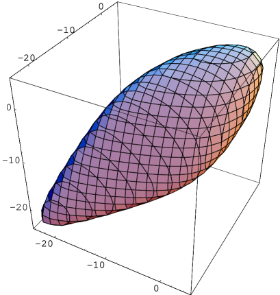
Figure 8: Terms which contribute to contribute to $\tilde{\Sigma}(p)$, with $h=0.4$ and $m=p=1$, by more than 1 part in $10^{10}$ are plotted. To evaluate the sum efficiently, we must focus on $\{k_{1},k_{2},k_{3}\}$ inside this volume.

In general, we are faced with the task of computing an $N$-dimensional infinite sum. For the case of diagrams which contribute to the propagator, the general term has the form of equation (38), and the overall sum can be written

$$I_{{\Lambda h}}(p) = \sum_{k}f(k_{1},\cdots,k_{n})$$ (50)

$$= \sum_{k_{1}}\left[\cdots\left[\sum_{k_{N}}f(k_{1},\cdots,k_{n})\right]\cdots\right],$$

where $f$ implicitly depends on $m$, $p$, $\Lambda$ and $h$. We have focused on the renormalized sunset diagram, but the following discussion is also applicable to the case with finite $\Lambda$. When computing the sums which represent Feynman integrals, it may not be practical to determine a priori which $\{k_{1},\cdots,k_{N}\}$ are significant. Consequently, we have developed a simple algorithm that evaluates $I_{{\Lambda h}}$ by dynamically tracking the size of the general term as a proportion of the “running total” for each of the $N$ nested sums in the overall sum. The precise criteria used to select the significant terms must be determined heuristically. The truncation error must be watched carefully, as all the terms in $I_{{\Lambda h}}$ are positive, and truncating the sum always underestimates $I_{{\Lambda h}}(p)$. The volume of $\{k_{1},k_{2},k_{3}\}$ space which contributes to $\tilde{\Sigma}(p)$ is shown in fig. (8).

The $k_{i}$ only appear in $f(k_{1},\cdots,k_{N})$ via the $c(k_{i})$ and $p(k_{i})$, defined in equations (22) and (23). Because $m^{2}$ (and $\Lambda^{2}$) does not change during the course of a given calculation, the $c(k)$ and $p(k)$ depend only on the integer values of the individual $k_{i}$. Thus we compute $c(k)$ and $p(k)$ for a range of $k_{i}$ and storing these results in arrays before starting on the evaluation of the sum itself. By using these stored values when the calculating the general term of the sum we avoid the need to recompute the exponentials in the $p(k)$ and $c(k)$ at every step.

We start each successive sum with an initial value of $k_{i}$ which maximized the general term for the previous sum. This is efficient since $k_{i-1}$ only differs by $\pm 1$ between the two cases, and the dependence of the general term on any of the $k_{i}$ is sufficiently weak to ensure that we are starting close to the maximal value. The one drawback to this approach is that when computing the final terms in the sum, we are adding small numbers to a large one (the “running total” for the overall sum), a circumstance that can lead to a loss of accuracy in fixed precision arithmetic. We have ensured we are not losing accuracy in this way by spot-checking our results with quadruple-precision arithmetic, but in a more sophisticated code this issue would be addressed more elegantly.

In the case of the sunset diagram, evaluating equation (44) with $h=0.4$ takes around 3 seconds of workstation CPU time, and the final result differs from the exact value determined from equation (45) by 1 part in $10^{10}$. For $h=0.6$, the accuracy drops to a few parts in $10^{8}$, and the execution time drops by around a factor of 3. For the specific case of the sunset diagram, considerable progress can be made with the analytic evaluation of the Feynman integral and this knowledge can be used to produce numerical values for $\tilde{\Sigma}(p)$. However, when compared to other methods for numerically evaluating integrals, the convergence properties and speed of the Sinc function method is impressive, involving as it does the direct numerical evaluation of a triple integral.

5.2 Improvements to Convergence

While simply adding up all the terms larger than a given minimum size is the most obvious way to evaluate an infinite sum, it is not necessarily the most efficient. In this initial paper we will give only a brief survey of techniques that could improve the convergence of the sums. In general, we foresee three broad classes of technique for improving convergence; analytical manipulations of the infinite sum’s general term (e.g. [13]), numerical extrapolations of successive partial sums (e.g. [14, 2]), and methods that effectively reduce the order of the $N$ dimensional sums generated by the Sinc function Feynman rules.

We will not attempt analytical rearrangements or evaluations of the sums we have derived. However, an interesting line of enquiry would be to consider whether known analytical treatments of Feynman integrals have analogous results which can be used to evaluate at least some of the infinite series in the $I_{{\Lambda h}}$. We do consider one example of the other two techniques - namely using extrapolation to speed the evaluation of the innermost sums, and generating a “dictionary” of pre-computed values from which the innermost sum can be accurately interpolated.

5.2.1 Aitken Extrapolation

For a general $I_{{\Lambda h}}$, if any one of the $k_{i}$ is becomes large and positive, the general term is dominated by factor like $\exp(-e^{k_{i}h})$. This expression decreases so precipitously that the transition between terms which are significant and those which are negligible is very sharp, and there is little to be gained from extrapolative techniques. However, for $k_{i}\ll 0$, the general term takes on a power-law behavior, whose regularity can be exploited by extrapolation. The general term of the sum is shown (for $k_{1}=k_{2}=k_{3}$) in fig. (9).

Figure 9: The general term of the Sinc integral form of the sunset diagram is shown, for $h=0.4$, $m=p=1$ and $k_{1}=k_{2}=k_{3}=k$. The general term decays like a power-law as $k$ becomes large and negative.

As a specific example of numerical extrapolation methods, consider the Aitken $\delta^{2}$ approach [2], which is applicable to infinite series whose general term behaves like $\sim x^{k}$ for large $k$, which is true of our problem when $k_{i}$ is decreasing. For a general infinite series with three successive partial sums $S_{n-1},S_{n},S_{n+1}$, Aitken’s $\delta^{2}$ method gives the improved estimate,

$$S^{\prime}=S_{n+1}-\frac{(S_{n+1}-S_{n})^{2}}{S_{n+1}-2S_{n}+S_{n-1}}.$$ (51)

If the general term of the series is $f(n)$, we can rewrite this as

$$S^{\prime}=S_{n+1}+\frac{f(n+1)^{2}}{f(n)-f(n+1)}.$$ (52)

Written in this form, we can recognize the general result for a sum of the type $\sum_{k=n}^{\infty}x^{n}$, with $f(n)=x^{n}$. For the specific case of the sunset diagram, using the Aitken $\delta^{2}$ extrapolation as $k_{3}$ becomes large and negative can improve the performance of the algorithm by at least $25\%$.

5.2.2 Reduction of Order

As we noted in the previous section, the Sinc function Feynman rules yield an $N$-dimensional infinite sum, where $N$ is the number of internal lines in the diagram. Consequently, if we can reduce the dimension of the infinite sum, we can expect a significant improvement in efficiency. By considering the general form of the sums derived from the Sinc function Feynman rules, we can see that while the overall sum is $N$-dimensional, the summand can typically be specified by fewer than $N$ independent parameters. In general, the sums take the form

$$I_{{\Lambda h}} = \sum_{k_{1}}\cdots\sum_{k_{j}}\sum_{k_{j+1}}\cdots\sum_{k_{N}}p(k_{1})\cdots p(k_{N})\times$$ (53)

$$\qquad f(d_{1},\cdots,d_{p},d_{p+1},\cdots,d_{q}).$$

Rearranging the $k_{i}$ so that $\{k_{j+1},\cdots,k_{N}\}$ only appear in a subset, $\{d_{p_{1}},\cdots,d_{q}\}$ of $\{d_{1},\cdots,d_{q}\}$, we can write the innermost $N-j$ sums as a function of $\{d_{1},\cdots,d_{p}\}$, $F(d_{1},\cdots,d_{p})$, where

$$F(d_{1},\cdots,d_{p}) = \sum_{k_{j}+1}\cdots\sum_{k_{N}}p(k_{j+1})\cdots p(k_{N})\times$$ (54)

$$\qquad f(d_{1},\cdots,d_{p},d_{p+1},\cdots,d_{q}).$$

Consequently, our sum is now

$$I_{{\Lambda h}}=\sum_{k_{1}}\cdots\sum_{k_{j}}p(k_{1})\cdots p(k_{j})F(d_{1},\cdots,d_{p}).$$ (55)

This may not seem like an improvement, since we still have to evaluate the $F(d_{1},\cdots,d_{p})$. However, by evaluating $F$ for a range of values of $\{d_{1},\cdots,d_{p}\}$ we can construct an interpolation table which will yield $F$ to some specified accuracy. Constructing the interpolation table will typically require $\exp{(c^{\prime}(N-j+q-p)}$ operations, while the evaluation of the remaining outermost sums will take a further $\exp{(c^{\prime\prime}j)}$ operations. Provided $N-j+p-q$ is less than $N$, the combined process will most likely be more efficient than evaluating the $N$ dimensional sum directly.

We now illustrate this process by the applying it to the increasingly familiar sunset diagram. If we focus on the renormalized quantity $\tilde{\Sigma}$, we can write equation (44) as

$$\tilde{\Sigma}_{h}(p)=\frac{m^{2}h^{3}}{(4\pi)^{4}}\sum_{k_{1},k_{2}}p(k_{1})p(k_{2})F(d)$$ (56)

where

$$F(d) = \sum_{k_{3}}\frac{p(k_{3})}{\left(d+1/c(k_{3})\right)^{2}}\ \left[\exp{\left(\frac{-p^{2}}{m^{2}}\frac{1}{d+1/c(k_{3})}\right)}\right.$$ (57)

$$\qquad\left.-1+\frac{p^{2}}{m^{2}}\frac{1}{d+1/c(k_{3})}\right],$$

$$d = \frac{1}{c(k_{1})}+\frac{1}{c(k_{2})}.$$ (58)

In practice, by computing $F(d)$ for several hundred values of $d$ we calculate $\tilde{\Sigma}(p)$ to within several parts in $10^{10}$ (with $h=0.4$) in less than 1/5th of the time needed for the direct evaluation of the three dimensional sum.

Another way to speed the evaluation of the diagrams would be to exploit the symmetry properties of the sums themselves, which reflects the structure of the underlying diagram. For instance, for a given $\{k_{1},k_{2},k_{3}\}$ the value of the general term in $\tilde{\Sigma}_{h}$ is not changed by permuting the $k_{i}$. By using this knowledge it would be possible to reduce the number of distinct sets of ${k_{1},k_{2},k_{3}}$ for which the general term in the sum had to be computed.

loop3 (150,75) thick i1 fermion,label=$p$i1,v1 fermion,label=$p$v3,o1 vanilla,left,tension=.4v1,v2,v1 vanilla,left,tension=.4v3,v2,v3 vanilla,left,tension=.2v1,v3 o1 v3

Figure 10: The three loop diagram that contributes to the $\lambda\phi^{4}$ propagator, with momentum, $p$.

Figure 11: We plot $\Sigma_{{\Lambda h}}^{(3)}(p)$ for $h=0.8$, $m=1$ and $\Lambda^{2}=16$. The prefactor of $m^{2}/(4\pi)^{6}$ in equation (60) has been removed from these numerical results.

5.3 Higher Order Diagrams

Until now, we have used the sunset diagram to illustrate the Sinc function approach to Feynman integrals. However, our aim is to develop a method which applies to arbitrary topologies. We now evaluate several specific higher order diagrams, although for convenience, we focus on contributions to the two-point function.

These diagrams typically contain sub-divergences, so we cannot regularize them using the prescription we employed with the sunset diagram. In order to focus on the Sinc function method itself, in this initial paper we use an explicit cut-off to render the higher order diagrams finite, and compare the Sinc function results to Monte Carlo integrations performed with the VEGAS algorithm [1, 2].

5.3.1 Case Study II: Third Order

Consider the following three loop graph,

$$\Sigma^{(3)}(x_{1}-x_{2})=\int d^{4}yG(x_{1}-y)^{2}G(x_{2}-y)^{2}G(x_{1}-x_{2}),$$ (59)

whose topology is illustrated in fig. (10). Applying the Sinc function Feynman rules gives:

$$\Sigma_{{\Lambda h}}^{(3)}(p) = \frac{m^{2}h^{5}}{(4\pi)^{6}}\sum_{k}\frac{p(k_{1})\cdots p(k_{5})}{\left(d_{1}d_{2}+(d_{1}+d_{2})/c(k_{1})\right)^{2}}\times$$ (60)

$$\exp{\left(-\frac{p^{2}}{m^{2}}\frac{d_{1}+d_{2}}{d_{1}d_{2}+(d_{1}+d_{2})/c(k_{1})}\right)},$$

where

$$d_{1}=\frac{1}{c(k_{2})}+\frac{1}{c(k_{3})},\qquad d_{2}=\frac{1}{c(k_{4})}+\frac{1}{c(k_{5})}.$$ (61)

As with the sunset diagram, $h$ can be taken close to unity without inducing a large difference between $\Sigma_{\Lambda}^{(3)}$ and $\Sigma_{{\Lambda h}}^{(3)}$, and $\Sigma_{\Lambda}^{(3)}(p)$ can be evaluated to six or seven significant figures in approximately twenty seconds. Since we have no independent estimate of $\Sigma_{\Lambda}^{(3)}(p)$, we heuristically determine the number of significant figures in our result by varying both $h$ and the size of the largest discarded terms in the multiple sum. Hopefully, a more careful analysis will give an a priori understanding of the truncation error in the evaluation of the series, and the $h$ dependence of the error in $I_{{\Lambda h}}$.

The results obtained from equation (60) can be independently checked by using VEGAS to evaluate the five dimensional integral representation of $\Sigma_{\Lambda}^{(3)}$. As well as confirming the Sinc function calculation, this also allows us to compare the time required to evaluate the Sinc function representation with the Monte Carlo algorithm. We find that to obtain four or five significant figures of $\Sigma^{(3)}$ using VEGAS takes around 50 times longer than it took us to find seven significant figures of $\Sigma^{(3)}$ from $I_{{\Lambda h}}$.

We do not place wish to place too much weight on this comparison. In practice, it is very unlikely that any $I_{\Lambda}$ would be evaluated directly, as it is almost always possible to perform some analytical simplifications. On the other side of the ledger, we have also not attempted make analytical improvements to $I_{{\Lambda h}}$. Moreover, VEGAS is a mature and well-tested algorithm. Conversely, we are using a very simple approach to evaluate the $I_{{\Lambda h}}$, and the previous results suggest that a more sophisticated algorithm would significantly reduce the time needed to evaluate the sums. Finally, the $I_{\Lambda}$ are, in general, cut-off dependent, whereas one usually wishes to calculate cut-off independent quantities. These can be combinations of different $I_{\Lambda}$ and their derivatives, in the limit that $\Lambda\rightarrow\infty$. This process of extracting cut-off independent quantities is presumably similar for the Sinc function and integral forms, but will generally lead to both integrands and summands which are more complicated that those which appear in the $I_{\Lambda}$ and $I_{{\Lambda h}}$.

However, while they are based on an artificial comparison, these results do suggest that Sinc function methods may lead to an useful approach for evaluating Feynman diagrams, which is intrinsically faster than one which relies on the use of Monte Carlo integration. Moreover, any advantage will become more pronounced when significant levels of numerical precision are required.

loop4 (150,80) thick i1 fermion,label=$p$i1,v1 fermion,label=$p$v2,o1 vanillav1,v3,v2 75,70v4 45,40v1 105,40v2 vanilla,right,tension=0v1,v2,v1 o1 vanilla,left,tension=0v3,v4,v3 v4

Figure 12: A four loop diagram that contributes to the $\lambda\phi^{4}$ propagator, with momentum, $p$.

Figure 13: We plot $\Sigma_{{\Lambda h}}^{(4)}(p)$ for $h=0.9$, $m=1$ and $\Lambda^{2}=16$. As is the case with the 3-loop example we consider, this quantity is explicitly cut-off dependent, and we have suppressed the $m^{2}/(4\pi)^{8}$ prefactor that appears in the Sinc function representation.

5.3.2 Case Study III: Fourth Order

The final diagram we consider here is the four loop contribution to the propagator, shown in fig. (12), which can be represented as the following integral over propagators,

$$\Sigma^{(4)}(x_{1}-x_{2}) = \int d^{4}y_{1}d^{4}y_{2}G(x_{1}-x_{2})G(y_{1}-y_{2})^{2}\times$$ (62)

$$\qquad G(x_{1}-y_{1})G(x_{1}-y_{2})\times$$

$$\qquad G(x_{2}-y_{1})G(x_{2}-y_{2}).$$

It is again straightforward to apply the Sinc function Feynman rules and take the Fourier transform to find $\Sigma_{{\Lambda h}}^{(4)}(p)$, and the results of evaluating it for a specific set of $\Lambda$, $m$ and $p$ are shown in fig. (13).

In this case, VEGAS takes around 20 minutes to find a result to within 1 part in $10^{4}$, whereas the Sinc function method returns a value accurate to 1 part in $10^{6}$ in approximately five minutes. Again, the Sinc function approach outperforms VEGAS by around two orders of magnitude, although the seven-dimensional sum is appreciably more expensive to evaluate than the previous five-dimensional example.

6 Conclusions and Discussion

In this paper we have developed the Sinc function representation, which associates arbitrary Feynman integrals with multi-dimensional, infinite sums. The basis of this representation is an approximation to the propagator, derived using the theory of generalized Sinc functions. We have used the Sinc function representation to develop a new approach to numerically evaluating Feynman integrals. This method is simple to implement and is potentially faster than Monte Carlo algorithms, which are currently used to evaluate most Feynman integrals that cannot be performed analytically.

We presented three “case studies” which illustrate the properties of the Sinc function representation. Firstly, we evaluated the two loop sunset diagram, and compared the Sinc function representation to explicit evaluations of the corresponding integral. We showed that we can easily compute results that are accurate to within a few parts in $10^{10}$, and that for diagrams with no sub-divergences it is straightforward to extract regularization independent quantities from the Sinc function representation. We then evaluated representative third and fourth order diagrams from the propagator expansion of $\lambda\phi^{4}$ field theory.

For the three and four loop diagrams we evaluated, we contrasted the Sinc function representation with direct calculations of the corresponding integrals with VEGAS, showing that the Sinc function representation is significantly more efficient than VEGAS. This advantage increases as the desired level of accuracy is raised, and can easily amount to several orders of magnitude in execution time. However, this direct comparison between Monte Carlo and Sinc function methods is somewhat artificial since the quantities computed are cut-off dependent, and we did not attempt to analytically simplify the integrals (or the sums) before evaluating them. Consequently, it remains to be seen whether the Sinc function representation will speed up realistic calculations.

In order to test the Sinc function representation in practical situations, we plan to investigate a number of topics. We have already used the Sinc function representation to evaluate the three-loop master diagrams whose analytical properties are discussed in detail by Broadhurst [15]. In the course of this work [16] we explicitly extended the Sinc function representation to diagrams with massless lines, and reproduced the analytical values of the master diagrams to better than 1 part in $10^{10}$. In addition to describing a renormalization procedure for the Sinc function representation of arbitrary diagrams, our immediate priority is to include fermion and vector fields, and thus to evaluate diagrams from QED and electroweak theory. We have calculated several simple QED diagrams with Sinc function techniques [17], and we are currently working on the systematic application of the Sinc function representation to arbitrary QED diagrams.

We have used a straightforward procedure to evaluate the multi-dimensional sums derived from the Sinc function Feynman rules. In Section 4 we discussed a variety of approaches to speeding up the computation of the sums, and it is possible that the numerical performance of the Sinc function representation can be significantly improved. Moreover, we have not yet attempted to analytically simplify Sinc function representations before evaluating then numerically. Consequently, the CPU time we currently need to evaluate the sum only provides an upper limit on what can be achieved.

Obtaining the Sinc function representation for a specific topology amounts to evaluating one or more Gaussian integrals, and the process is easily automated with any computer algebra package. If the Sinc function representation is useful in realistic situations, we expect it will be straightforward to integrate it with existing tools for automatically evaluating diagrams. Moreover, applying the Sinc function Feynman rules to diagrams which contain several fields with different masses is no more complicated than evaluating the same topology with identical lines. Diagrams with more than two external lines also present no new difficulties, although in this case more than one Fourier transform is needed to move from coordinate to momentum space, since an $n$-point diagram has $n-1$ independent external momenta.

Strictly speaking the Sinc function representation is not just a “better way to do integrals”, since when evaluated to arbitrary precision, the Sinc function representation converges to an approximation to the integral, rather than the integral itself. However, this approximation can be made arbitrarily accurate, so in practice evaluating the Sinc function representation is equivalent to a direct computation of the integral. Moreover, several other approaches lead to expressions for Feynman integrals that are written as infinite sums [18, 19, 20, 21]. However, these methods yield expressions for the exact integrals, and are therefore not equivalent to the Sinc function representation.

While many approaches to numerical integration outperform Monte Carlo techniques in one or two dimensions, their efficiency scales typically very poorly with the dimension of the integral. For the integrals derived from Feynman diagrams, the Sinc function representation provides an exception to this general rule. For example, the 4th order diagram we studied can be expressed as a seven dimensional integral, but a Monte Carlo integration with VEGAS takes much longer than the Sinc function representation to achieve the same level of accuracy. The task before us now is to harness the mathematical properties of the Sinc function representation, and apply them to solving physical problems.

Appendix A Numerical Details

The numerical results described in this paper we all obtained on the same Sun workstation, with 250MHz Ultrasparc II CPUs. We refrain from giving precise timings, since these depend strongly on the specific combination of hardware and software, and the timings we do give reflect the use of aggressive compiler optimization settings. The codes are implemented in Fortran 77. Sample codes (including those used to perform the calculations described in this paper) are available at the following URL:
http://www.het.brown.edu/people/easther/feynman

References

- [1] G. P. Lepage, J. Comput. Phys. 27, 192 (1978).
- [2] W. Press, S. Teukolsky, W. Vetterling, and B. Flannery, Numerical Recipes in Fortran, 2 ed. (Cambridge UP, Cambridge, 1992).
- [3] T. Kinoshita, in Quantum Electrodynamics, edited by T. Kinoshita (World Scientific, Singapore, 1980), pp. 218–321.
- [4] R. Harlander and M. Steinhauser, hep-ph/9812357 (1998).
- [5] S. García, G. S. Guralnik, and J. W. Lawson, Phys. Lett. B 333, 119 (1994).
- [6] S. García, Z. Guralnik, and G. S. Guralnik, hep-th/9612079 (1996).
- [7] J. W. Lawson and G. S. Guralnik, Nucl. Phys. B 459, 589 (1996).
- [8] S. C. Hahn, Ph.D. thesis, Brown University, 1998.
- [9] S. C. Hahn and G. S. Guralnik, hep-th/9901019 (1999).
- [10] F. Stenger, Numerical Methods Based on Sinc and Analytic Functions (Springer Verlag, New York, NY, 1993).
- [11] J. R. Higgins, Bull A. M. S. 12, 45 (1985).
- [12] P. Ramond, Field Theory: A Modern Primer, 2 ed. (Addison Wesley, Redwood City, CA, 1989).
- [13] G. Arfken, Mathematical Methods for Physicists, 3 ed. (Academic Press, Orlando, 1985).
- [14] Handbook of Mathematical Functions, edited by M. Abramowitz and I. Stegun (Dover, New York, NY, 1965).
- [15] D. Broadhurst, Eur. Phys. J. C8, 311 (1999).
-
[16]
R. Easther, G. Guralnik, and S. Hahn,
hep-ph/9912255 (1999). - [17] W.-M. Wang, Perturbative calculations in quantum field theory, ScB Thesis, Brown University, 1998.
- [18] E. Mendels, Nuovo Cimento 45A, 87 (1978).
- [19] K. G. Chetyrkin, A. L. Kataev, and F. V. Tkachov, Nuc. Phys. B 174, 345 (1980).
- [20] A. E. Terrano, Phys. Lett. B 93, 424 (1980).
- [21] D. J. Broadhurst and D. Kreimer, Int. J Mod. Phys. C 6, 519 (1995).