Asymptotic Calculation of Discrete Nonlinear Wave Interactions

Abstract

We illustrate how to compute asymptotic interactions between discrete solitary waves of dispersive equations, using the approach proposed by Manton [Nucl. Phys. B 150, 397 (1979)]. We also discuss the complications arising due to discreteness and showcase the application of the method in nonlinear Schrödinger, as well as in Klein-Gordon lattices, finding excellent agreement with direct numerical computations.

1 Introduction

Solitary wave interactions and collisions are among the signature characteristics of such nonlinear coherent structures and have been extensively studied in both integrable and non-integrable dispersive nonlinear models [2, 3, 4, 5, 6, 7]. The relevant physical contexts where such phenomena may arise range from the more traditional areas of fluid mechanics and plasma physics (discussed in the above references) or high-energy physics [8] to nonlinear optics [9, 10], and the recently emerging applications of Bose-Einstein condensates [11, 12].

On the other hand, in the past decade there has been an explosive parallel evolution of the theory and applications of discrete nonlinear waves, namely discrete solitons and discrete breathers, see, e.g. [13] for a number of review papers on the topic. In this case, the applications refer to nonlinear waveguide arrays [14] and photorefractive crystals [15], to Bose-Einstein condensates in deep optical lattices [16], to the local denaturation of the DNA double strand [17], and to micro-mechanical cantilever arrays [18] among many others.

Our aim in the present work is to illustrate a technique for computing solitary wave interactions in discrete systems. We should mention here that for continuum systems, there exists a large variety of methods for computing such interactions. These range from the perturbation theoretical works of [19], to the variational methods of [20, 21, 22], the Fredholm-alternative based technique of [23] or the more rigorous calculations of [24] based on Lin’s method. In a recent publication [25], we took an alternative route to these methods, by implementing an asymptotic calculation using the approach proposed by Manton [26] (which, in turn, was generalizing the earlier work of  [27]). Performing such calculations in discrete systems is, however, considerably less straightforward. One of the complications is that, aside from the tail-tail interaction of the waves, each wave may also reside on a periodic substrate potential, usually termed the Peierls-Nabarro barrier [13]. As a result, except for the (typically exponential in the wave separation) tail-induced potential, a local potential may arise due to discreteness, resulting in a washboard potential structure which can be captured by variational techniques [21, 22].

In what follows, we show how to compute discrete solitary wave interactions by means of Manton’s method. We bypass the issue of the Peierls-Nabarro barrier by working with problems whose static solutions do not encounter such a barrier (so that they can be placed anywhere on the lattice). We demonstrate this approach both for breathers in nonlinear Schrödinger lattices – namely in its famous Ablowitz-Ladik (ALNLS) variant [28] – and for kinks in Klein-Gordon lattices – namely in a discrete version of the $\phi^{4}$ model, proposed in [29, 30, 31]. While the former model is integrable, integrability is not a key ingredient in our calculation. Instead, the existence of a discrete analog of momentum conservation law (and also the absence of the Peierls-Nabarro barrier) are indispensable for being able to carry through the Manton calculation as we show in the following sections. We compare our analytical results with direct numerical computations, finding excellent agreement between the two during the time interval in which the waves interact without losing their individual character. Furthermore, our calculations also capture the correct continuum limit (known from the earlier works of [20, 26]; see also [25]), as the lattice spacing $h\rightarrow 0$.

Our presentation is organized as follows. In section 2, we illustrate the method for the breathing solitons of the Ablowitz-Ladik model. In section 3, we compute the interaction potential for kinks in a non-integrable, discrete $\phi^{4}$ model. Finally, in section 4 we summarize our results and present our conclusions and some interesting directions for future study.

2 Soliton Interactions in the Ablowitz-Ladik Model

Similarly to the corresponding continuum calculation (see, e.g., [25] for such calculations in different models), the key to performing a calculation for the discrete case using Manton’s method is the existence of a momentum as a conserved quantity. In the ALNLS model, such a momentum operator is one of the integrals of motion (that is why integrability is desirable for performing such a calculation, even though, as we will show below, it is not a necessary condition), and has the form (see, e.g.,  [3, 32] for details)

$$P=i\sum_{n=-\infty}^{\infty}\left(\psi_{n}\psi_{n+1}^{\star}-\psi_{n}^{\star}\psi_{n+1}\right),$$ (1)

where $\psi$ is the complex field, and the star is used to denote complex conjugation. We will focus here on the ALNLS equation in the form [32]

$$i\dot{\psi}_{n}+(\psi_{n+1}+\psi_{n-1})(1+|\psi_{n}|^{2})=0,$$ (2)

with the explicit stationary soliton solution

$$\psi_{n}=\sinh(\beta){\rm sech}\left(\beta(n-s)\right)\exp(i\sigma),$$ (3)

where $\dot{\sigma}=2\cosh(\beta)$. Here the overdot denotes time derivative, $\beta$ is the inverse width of the pulse soliton and $s$ is the arbitrary position of the center of the pulse. We commence by examining in-phase solitons, but we will also relax this constraint later. Note that Eq. (2) has the lattice spacing $h$ scaled out, but it is straightforward to incorporate it and we will see how to relate it to the relevant continuum limit of $h\rightarrow 0$ for our calculations.

In the spirit of [26], we now consider two solitons, one centered at $0$ and one centered at $s\gg 0$, i.e., two widely-separated solitons. We compute $dP/dt$ by performing the summation over $n$ not for the infinite lattice (when the result would be zero due to the relevant conservation law), but rather from $n=M$ to $n=N$, with $M\ll 0$, and $0\ll N\ll s$. The idea behind this calculation is that, in fact, the force in this interval is not going to be zero, but rather would be finite due to the soliton-soliton interaction. When summing on the infinite line, as a result of Newton’s third law, the action of the first soliton on the second and the equal and opposite reaction of the second on the first cancel each other, thus resulting in zero net momentum gain. However, for a finite interval encompassing only one soliton, the amount of momentum gain is finite, due to the fact that the one soliton experiences the pull (or push) of the other soliton at the boundary of the interval where we perform the calculation. In precise mathematical terms, we evaluate:

$$\frac{dP}{dt} = -2\sum_{n=M}^{N}\left(|\psi_{n+1}|^{2}-|\psi_{n}|^{2}\right)$$ (4)

$$+ \sum_{n=M}^{N}\left(\psi_{n}\psi_{n+2}^{\star}+\psi_{n}^{\star}\psi_{n+2}\right)\left(1+|\psi_{n+1}|^{2}\right)$$

$$- \sum_{n=M}^{N}\left(\psi_{n-1}\psi_{n+1}^{\star}+\psi_{n-1}^{\star}\psi_{n+1}\right)\left(1+|\psi_{n}|^{2}\right).$$

However, observing the telescopic nature of the sums in the right hand side (RHS) of Eq. (4), we infer that

$$\frac{dP}{dt} = -2\left(|\psi_{N+1}|^{2}-|\psi_{M}|^{2}\right)$$ (5)

$$+ \left(\psi_{N}\psi_{N+2}^{\star}+\psi_{N}^{\star}\psi_{N+2}\right)\left(1+|\psi_{N+1}|^{2}\right)$$

$$- \left(\psi_{M-1}\psi_{M+1}^{\star}+\psi_{M-1}^{\star}\psi_{M+1}\right)\left(1+|\psi_{M}|^{2}\right).$$

As usual in Manton’s method, and based on intuitive physical arguments, the main contribution in this asymptotic calculation stems from the boundary between the two solitons. Hence, we drop the terms with subscript $M$ and only consider the contributions with subscript $N$ in what follows.

We then invoke the soliton ansatz

$$\psi_{n}=\psi_{n}^{(1)}+\psi_{n}^{(2)}$$ (6)

with $\psi_{n}^{(1)}=\sinh(\beta){\rm sech(\beta n)}\exp(i\sigma)$ and $\psi_{n}^{(2)}=\sinh(\beta){\rm sech(\beta(n-s))}\exp(i\sigma)$ (i.e., two in-phase solitons). Since $0\ll N\ll s$, we can use the asymptotic form of the soliton tail at $n=N$, according to

$$\psi_{n}^{(1)}=2\sinh(\beta)\exp(-\beta N)\exp(i\sigma)\,,$$ (7)

$$\psi_{n}^{(2)}=2\sinh(\beta)\exp(\beta(N-s))\exp(i\sigma)\,.$$ (8)

Substituting the ansatz of Eq.  (6) and the expressions in Eqs. (7)-(8) into Eq. (5), and computing the terms arising from the soliton-soliton interaction, we obtain that

$$\frac{dP}{dt}\approx 32\sinh^{4}(\beta)\exp(-\beta s)\,.$$ (9)

We note a number of comments on this calculation.

• Equation of motion for $s(t)$: As explained in [25], in order to obtain the equation of motion for the inter-soliton separation $s(t)$, we can use Newton’s equation in the form

  $$M_{s}\ddot{s}=-2\frac{dP}{dt}\,,$$ (10)

  where $M_{s}$ is the mass of the soliton; the factor “$2$” comes from the fact that there is an equal and opposite pull (or push) on the second soliton, and hence their relative distance decreases by twice the contribution of $dP/dt$ to each of them; and finally the unfamiliar “–” sign originates from the fact that a positive boundary contribution to $dP/dt$ decreases the soliton distance, while the opposite is true for a negative $dP/dt$. In the present case, the soliton mass is given by  [32]

  $$M_{s}=\sum_{n=-\infty}^{\infty}{\rm ln}\left(1+|\psi_{n}|^{2}\right)=2\beta$$ (11)

  (once again, a direct benefit of integrability being the immediate accessibility of the relevant conservation law). Then one can straightforwardly infer the equation for $s(t)$ as

  $$\ddot{s}=-\frac{32}{\beta}\sinh^{4}(\beta)\exp(-\beta s)\,,$$ (12)

  while the relevant effective soliton interaction potential (for a unit mass particle) is

  $$V(s)=-\frac{32}{\beta^{2}}\sinh^{4}(\beta)\exp(-\beta s)\,.$$ (13)

  We have examined the validity of the pertinent calculation by studying numerically the two-soliton collisions in the ALNLS model. Typical results are illustrated in Fig. 1 for $\beta=2$ and two solitons initialized at a distance of $s(0)=10$ between them. The upper panel of the figure shows the numerical (solid line) versus theoretical (dashed line) prediction for the soliton separation as a function of time, $s(t)$, revealing excellent agreement for all times until about $t\approx 657$, when the separation becomes $s<3$ and the solitons can no longer be characterized as individual entities; hence, it is reasonable that our asymptotic calculations fail at that point. In fact, it appears that the analytical calculation gives a very good agreement with the numerics well past the point where we might have anticipated such agreement (on the basis of our expansion assumptions), and approximately even up to the collision point.

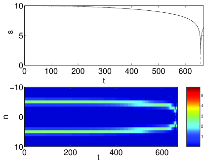
  Figure 1: The top panel shows the soliton-soliton separation as a function of time, $s(t)$, for the numerical integration of the ALNLS equation with two superposed solitons (at $n=-5$ and $n=5$) as the initial condition. The solid line yields the numerical result (calculated by obtaining independently the center of mass of the left and right pulse in the configuration, and subtracting the former from the latter), while the dashed line provides our asymptotic prediction of Eq. (12). Note the excellent agreement between the two, essentially up to the collision time, since the two curves cannot be distinguished, practically, up to that time. The bottom panel shows the space-time contour plot of the “local mass” $m_{n}={\rm ln}(1+|\psi_{n}|^{2})$, clearly illustrating the evolution towards the collision of the center of mass of the two solitons.

• Role of the soliton relative phase: In order to examine it, it is simple to impart to one of the ALNLS solitons a free phase $\exp(i\phi)$, with respect to the other soliton. In this case, the results of Eqs. (12)-(13) are retrieved, but with the RHS expression multiplied by $\cos(\phi)$. This is rather natural as in-phase ALNLS solitons are expected to attract each other, while out-of-phase ones are expected to experience mutual repulsion [20, 21, 22].

• Retrieving the continuum limit: In the continuum limit, one should recover the relevant expression of [33] (see also [25]). In reshaping our expression to match the latter, we observe that in the continuum limit the discrete spacing $s$ will appropriately renormalize to the continuum spacing, while $\sinh(\beta)\rightarrow\beta$ for the continuum soliton. Finally, our prefactor of $32$ in Eq. (9) will match the corresponding prefactor of $8$ in [25, 33], since the momentum is defined with a factor of $1/2$ (as in Eq. (11) of  [25]) and there is an extra factor of $1/2$ multiplying the RHS of Eq. (2) to match it with the (continuum limit of the) RHS of the equations used in [25, 33].

3 Kink Interactions in a Discrete $\phi^{4}$ Model

We consider now a rather different class of models, namely Klein-Gordon lattices. In particular, we focus on a discretization of the $\phi^{4}$ field theory of the form:

$$\ddot{u}_{n}=C\Delta_{2}u_{n}+2u_{n}-u_{n}^{2}(u_{n+1}+u_{n-1}),$$ (14)

where $C=1/h^{2}$ is the coupling parameter and $\Delta_{2}u_{n}=(u_{n+1}+u_{n-1}-2u_{n})$ stands for the discrete Laplacian. This type of discretization for the RHS was discussed in [29] (motivated by ODE examples), and independently rediscovered for the $\phi^{4}$ field theory in [30, 31]. An interesting feature of the model is that, while non-integrable, it possesses exact solitary wave solutions in the form

$$u_{n}=\tanh(\alpha(n-s)),$$ (15)

where $s$ denotes the center of the kink, $\alpha$ is the inverse width of the kink and $\cosh(2\alpha)=(1+h^{2})/(1-h^{2})$. This feature, while useful, is again not an indispensable one for the development of the Manton procedure. In fact, the only related property that is necessary for the calculation is the exponential tail of the solitary waves (which can, in fact, be derived by an appropriate exponential tail ansatz, even if it is not explicitly available in the form of an analytical solution).

Another property of this model, more crucial for our considerations, is that it possesses a discrete analog of the continuum momentum conservation law. In particular, as shown in [30], the relevant momentum is of the form:

$$P=-\frac{1}{2}\sum_{n=-\infty}^{\infty}\dot{u}_{n}\left(u_{n+1}-u_{n-1}\right)\,.$$ (16)

One can then perform a similar calculation of $dP/dt$ summing from $n=M$ to $n=N$, thus obtaining:

$$\frac{dP}{dt}=-\frac{1}{2}\sum_{n=M}^{N}\left[H(u_{n+1},u_{n})-H(u_{n},u_{n-1})+\dot{u}_{n}\dot{u}_{n+1}-\dot{u}_{n-1}\dot{u}_{n}\right],$$ (17)

where

$$H(u_{n+1},u_{n})=C\left(u_{n+1}-u_{n}\right)^{2}+2u_{n}u_{n+1}-u_{n}^{2}u_{n+1}^{2}\,.$$ (18)

Given the telescopic nature of the summation, we can easily infer that

$$\frac{dP}{dt}=-\frac{1}{2}\left[H(u_{N+1},u_{N})-H(u_{M},u_{M-1})+\dot{u}_{N}\dot{u}_{N+1}-\dot{u}_{M-1}\dot{u}_{M}\right]\,.$$ (19)

We now use the kink-antikink ansatz of the form (see also [25, 26])

$$u_{n}=u_{n}^{(1)}+u_{n}^{(2)}+r\,,$$ (20)

where $r$ is the value of the inhomogeneous background steady state on which the kinks exist. In the case of the $\phi^{4}$ model, it can be easily inferred that $r=\pm 1$. Without loss of generality we use $r=-1$ here. The asymptotic form of the kink profiles, using the expression of Eq. (15) at $n=N$, will be:

$$u_{N}^{(1)}=1-2\exp(-2\alpha N)\,,$$ (21)

$$u_{N}^{(2)}=1-2\exp\left(2\alpha(N-s)\right)\,.$$ (22)

Notice that in general the first term in the RHS of Eqs. (21)-(22) is $-r$.

Using the ansatz of Eq. (20) along with Eqs. (21)-(22) in the expression of Eq. (19), and isolating the contributions stemming from the tail-tail interaction (to leading order, once again coming solely from $n=N$), we obtain that

$$\frac{dP}{dt}\approx 16\exp(-2\alpha s)\left[C\sinh^{2}(\alpha)+\cosh^{2}(\alpha)\right]\,.$$ (23)

We again make a number of comments on the calculation.

• Equation of motion for $s(t)$: In this model, we do not have an immediately available definition of the soliton mass $M_{s}$. However, considering the momentum itself, we realize that using a time dependent center of mass $s(t)$ for the position of the center of one of the solitons, and substituting that along with Eq. (15) in Eq. (16), we obtain

  $$P=\alpha\dot{s}\sum_{n=-\infty}^{\infty}{\rm sech}^{2}(\alpha(n-s))\left[\tanh\left(\alpha(n+1-s)\right)-\tanh\left(\alpha(n-s)\right)\right]\,.$$ (24)

  Since $\alpha$ is an effective spacing parameter that will be used to renormalize the distance in the continuum limit (see below), we will consider the expression multiplying $\alpha\dot{s}$ in the above formula of the momentum as the mass of the kink $M_{k}$. $M_{k}$ and $\alpha$ have been computed numerically for various spacings $h$ in the interval $(0,1)$ and are shown in Fig. 2. It can be clearly observed that $M_{k}$ tends to its continuum limit of $4/3$ ($=\int_{-\infty}^{\infty}u_{x}^{2}dx=\int_{-\infty}^{\infty}{\rm\rm sech(x)}^{4}dx$), validating the usefulness of this definition. Note also in the same graph that the behavior of $\alpha$ is linear in $h$ for small enough $h$ (in fact, the relevant Taylor expansion is $\alpha\approx h+h^{3}/3+\dots$ for small $h$). Let us also mention that while the expression of Eq. (15) for the exact solution appears to be necessary for the computation of the kink mass from Eq. (24), this constraint can be relaxed as well. For instance, one can quite efficiently approximate the mass numerically (see also our numerical calculations below).

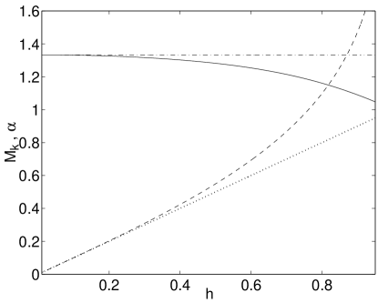
  Figure 2: The graph shows the dependence of the kink mass $M_{k}$ given by Eq. (24) (solid line) as a function of the lattice spacing $h$. The continuum limit corresponding to $M_{k}=4/3$ (see the main text) is shown by the dash-dotted line. The dashed line illustrates the dependence of the parameter $\alpha$ on the spacing $h$, while the dotted line shows the linear behavior for comparison.

  Equating the right hand side expression from the momentum of Eq. (23) [doubled and with a minus sign for reasons similar to those mentioned previously for Eq. (10)], with the expression stemming from the time derivative of $P=\alpha\dot{s}M_{k}$, we obtain the evolution dynamics

  $$\ddot{s}=-\frac{32\exp(-2\alpha s)}{M_{k}\alpha}\left[C\sinh^{2}(\alpha)+\cosh^{2}(\alpha)\right].$$ (25)

  The relevant effective tail-tail kink-antikink interaction potential (for a unit mass particle) can then be obtained in the form

  $$V(s)=-\frac{16\exp(-2\alpha s)}{\alpha^{2}}\left[C\sinh^{2}(\alpha)+\cosh^{2}(\alpha)\right]\,.$$ (26)

  These predictions are tested against numerical simulations, obtaining once again excellent agreement almost up to the collision point (the two trajectories only separate visibly for $t\approx 45$, when the distance of the kink and anti-kink is less than 5 sites). The results are illustrated in Fig. 3.

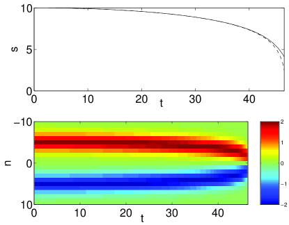
  Figure 3: Same as Figure 1, but now for the kink-antikink interaction of the $\phi^{4}$ model for $h=0.5$. The bottom panel shows the space-time contour plots of the quantity $D_{n}=u_{n+1}-u_{n-1}$ whose square we used for our local (approximate) calculation of the centers of mass of the two kink and antikink, respectively.

• Retrieving the continuum limit: In the continuum limit, we have to compare Eq. (23) with the expression for $dP/dt$ that was obtained in [26],

  $$\frac{dP}{dt}\approx 2A^{2}m^{2}\exp(-ms)\,,$$ (27)

  for two solitons with the asymptotic form

  $$u^{(1)} = -r+A\exp(-mx),$$ (28)

  $$u^{(2)} = -r+A\exp(m(x-s)).$$ (29)

  Hence, when renormalizing the distance $x$ by our $\alpha$ close to the continuum limit of $h\rightarrow 0$, and with $m=2$ and $A=-2$, one obtains $dP/dt\approx 32\exp(-2s)$ for the $\phi^{4}$ field theory. We retrieve this result from the expression of Eq. (23), since $\lim_{h\rightarrow 0}C(\sinh(\alpha))^{2}=1$ and $\cosh(2\alpha)\rightarrow 1$ as $h\rightarrow 0$, by a straighforward limit in the expression defining $\alpha$ (just below Eq. (15)). Once again, the correct continuum limit is obtained from the discrete expression as a special case.

4 Conclusions

In this work, we have presented a self-contained description of the way to use the technique first proposed by Manton in [26] for the continuum Klein-Gordon models, in order to quantify tail-tail interactions of soliton solutions of discrete, dispersive nonlinear wave equations. We demonstrated the calculation via two prototypical examples, one in the form of soliton-soliton interactions in the completely integrable Ablowitz-Ladik model and one in the form of kink-antikink interactions in a (non-integrable) Klein-Gordon chain. We highlighted the key necessary ingredients for carrying out such a calculation, namely the existence of a momentum-like quantity which is conserved due to its “telescopic property”. This allows, similarly to the continuum limit, to arrive at an expression involving only boundary terms when computing the force exerted on a fraction of the lattice encompassing one of the two solitary waves. Assessing the leading order contribution from these surface terms and equating it (with appropriate prefactors taking into consideration the total magnitude and direction of the relative change of displacement of the two waves) to the particle-like momentum of the coherent structures, we obtain the kinematics of their relative displacement. The relevant expression clearly highlights the exponential nature of the tail-tail interactions (which is natural, given the exponential tails of the solitary waves). The obtained expressions have been tested both against the limiting case of their continuum counterparts which were previously available, and against direct numerical simulations, providing excellent agreement with the direct numerical experiments, practically up to the wave collision point (for the attractive interactions considered herein).

The success of our predictions against the corresponding numerical simulations naturally raises the question of generalizations, as well as limitations of the technique. The most significant limitation is that “standard” discretizations often defy the existence of a momentum conservation law, and do not share such a property with their continuum siblings, restraining themselves to the integer shift invariance, rather than an effective continuum-like translational invariance. It then takes either integrable (such as e.g. the ones of [28]) or “non-standard” (see e.g. [30, 31] and references therein) discretizations to circumvent this difficulty and possess a discrete analog of the momentum. Hence, it would be very desirable to be able to extend our considerations to cases where the momentum conservation is absent, hopefully obtaining, in addition to the tail-tail terms already captured above, the ones from the local, periodic Peierls-Nabarro barrier. Another natural extension of the Manton approach (in fact, both in the continuum and in the discrete systems) would be the study of its multi-dimensional analog. While by no means straightforward (especially given the sparsity of analytically available solutions and the difficulty of questions such as the definition of the right momentum/contour), it constitutes an increasingly relevant generalization of the considerations presented herein. Work along these directions is currently underway and will be reported in future publications.

This work was supported in part by the U.S. Department of Energy. PGK is grateful to the Eppley Foundation for Research, the NSF-DMS-0204585, NSF-DMS-0505063 and the NSF-CAREER program for financial support and to the Center for Nonlinear Studies of Los Alamos National Laboratory for its hospitality. I.B. acknowledges support of the Swiss National Science Foundation and the Center for Nonlinear Studies of Los Alamos National Laboratory for its hospitality.

References

References

- [1]
- [2] P.G. Drazin and R.S. Johnson, Solitons: an introduction (Cambridge University Press, Cambridge, U.K., 1989).
- [3] M.J. Ablowitz and H. Segur, Solitons and the Inverse Scattering Transform (SIAM, Philadelphia, 1981).
- [4] E. Infeld and G. Rowlands, Nonlinear Waves, Solitons and Chaos (Cambridge University Press, Cambridge, 1990).
- [5] R.K. Dodd, J.C. Eilbeck, J.D. Gibbon and H.C. Morris, Solitons and Nonlinear Waves (Academic Press, London, 1982).
- [6] A. Scott, Nonlinear Science (Oxford University Press, New York, 1999).
- [7] M. Remoissenet, Waves Called Solitons, (Springer-Verlag, Berlin 1999).
- [8] T.I. Belova, A.E. Kudryavtsev, Usp. Fiz. Nauk, 167, 377 (1997) [Physics-Uspekhi, 40, 359 (1997)].
- [9] A. Hasegawa and Y. Kodama, Solitons in Optical Communications, (Clarendon Press, Oxford 1995).
- [10] Y.S. Kivshar and G.P. Agrawal, Optical Solitons: From Fibers to Photonic Crystals (Academic, San Diego, 2003).
- [11] L. P. Pitaevskii and S. Stringari, Bose Einstein Condensation (Clarendon Press, Oxford, 2003).
- [12] K.E. Strecker, G.B. Partridge, A.G. Truscott, and R.G. Hulet, Nature 417, 150 (2002).
- [13] D. Campbell, S. Flach and Y.S. Kivshar, Phys. Today 57, 43 (2004); J.Ch. Eilbeck and M. Johansson, in Localization and Energy Transfer in Nonlinear Systems, L. Vazquez, R.S. MacKay, and M.P. Zorzano (eds.), (World Scientific, Singapore, 2003), p.44; P.G. Kevrekidis, K.Ø. Rasmussen, and A.R. Bishop, Int. J. Mod. Phys. B 15, 2833 (2001); S. Flach and C.R. Willis, Phys. Rep. 295, 181 (1998); S. Aubry, Physica D 103, 201 (1997); D. Hennig and G. Tsironis, Physics Reports 307, 333 (1999).
- [14] D.N. Christodoulides, F. Lederer and Y. Silberberg, Nature 424, 817 (2003).
- [15] N.K. Efremidis, S. Sears, D.N. Christodoulides, J.W. Fleischer and M. Segev, Phys. Rev. E 66, 046602 (2002); J.W. Fleischer, T. Carmon, M. Segev, N.K. Efremidis and D.N. Christodoulides, Phys. Rev. Lett. 90, 023902 (2003); J.W. Fleischer, M. Segev, N.K. Efremidis and D.N. Christodoulides, Nature 422, 147 (2003).
- [16] V.A. Brazhnyi and V.V. Konotop, Mod. Phys. Lett. B 18, 627 (2004); P.G. Kevrekidis and D.J. Frantzeskakis, Mod. Phys. Lett. B 18, 173 (2004).
- [17] See e.g. S. Ares, N.K. Voulgarakis, K.Ø. Rasmussen and A.R. Bishop, Phys. Rev. Lett. 94, 035504 (2005); G. Kalosakas, K.Ø. Rasmussen, A.R. Bishop, C.H. Choi and A. Usheva, Europhys. Lett. 68, 127 (2004) and references therein.
- [18] M. Sato and A.J. Sievers, Nature 432, 486 (2004); M. Sato, B. E. Hubbard, A. J. Sievers, B. Ilic, D. A. Czaplewski, and H. G. Craighead, Phys. Rev. Lett. 90, 044102 (2003).
- [19] V.I. Karpman and V.V. Solov’ev, Phys. D 3, 142 (1981); V.I. Karpman and V.V. Solov’ev, Phys. D 3, 487 (1981).
- [20] B.A. Malomed, Progress in Optics 43, 69 (2002); B.A. Malomed, Phys. Rev. E 58, 7928 (1998).
- [21] T. Kapitula, P. G. Kevrekidis, and B. A. Malomed, Phys. Rev. E 63, 036604 (2001).
- [22] R. Carretero-González and K. Promislow, Phys. Rev. A 66, 033610 (2002) and references therein.
- [23] C. Elphick, E. Meron, and E.A. Spiegel, SIAM J. Appl. Math. 50, 490 (1990).
- [24] B. Sandstede, Trans. Amer. Math. Soc. 350, 429 (1998).
- [25] P.G. Kevrekidis, Avinash Khare and A. Saxena, Phys. Rev. E 70, 057603 (2004).
- [26] N.S. Manton, Nucl. Phys. B 150, 397 (1979).
- [27] J.N. Goldberg, P.S. Jang, S.Y. Park, and K.C. Wali, Phys. Rev. D 18, 542 (1978); J.K. Perring and T.H.R. Skyrme, Nucl. Phys. 31, 550 (1962); R. Rajaraman, Phys. Rev. D 15, 2866 (1977).
- [28] M.J. Ablowitz and J.F. Ladik, J. Math. Phys. 16, 598 (1975); M.J. Ablowitz and J.F. Ladik, J. Math. Phys., 17, 1011 (1976).
- [29] C.M. Bender and A. Tovbis, J. Math. Phys. 38, 3700 (1997).
- [30] P.G. Kevrekidis, Physica D 183, 68 (2003).
- [31] F. Cooper, A. Khare, B. Mihaila, and A. Saxena, Phys. Rev. E 72, in press (2005); nlin.SI/0502054.
- [32] D. Cai, A.R. Bishop and N. Grønbech-Jensen, Phys. Rev. E 53, 4131 (1996).
- [33] V.V. Afanasjev, B.A. Malomed, and P.L. Chu, Phys. Rev. E 56, 6020 (1997).