Foliations of Isonergy Surfaces and Singularities of Curves

Abstract.

It is well known that changes in the Liouville foliations of the isoenergy surfaces of an integrable system imply that the bifurcation set has singularities at the corresponding energy level. We formulate certain genericity assumptions for two degrees of freedom integrable systems and we prove the opposite statement: the essential critical points of the bifurcation set appear only if the Liouville foliations of the isoenergy surfaces change at the corresponding energy levels. Along the proof, we give full classification of the structure of the isoenergy surfaces near the critical set under our genericity assumptions and we give their complete list using Fomenko graphs. This may be viewed as a step towards completing the Smale program for relating the energy surfaces foliation structure to singularities of the momentum mappings for non-degenerate integrable two degrees of freedom systems.

1. Introduction

A decade ago, at his International Congress of Mathematics address [49], Juergen Moser concluded his lecture with the following remark:

“Most striking to me is the development of integrable systems (over 30 years ago) which did not grow out of any given problem, but out of phenomenon which was discovered by numerical experiments in a problem of fluid dynamics”.

Indeed, Moser provides examples in these notes showing that the structure of integrable systems is both surprisingly rich and surprisingly relevant for the analysis of systems arising in nature. Moser’s mainly concentrated in these notes on the richness of infinite dimensional integrable systems. It is a great honor for us to contribute to this issue in his memory, a description of the rich structure of integrable two degrees of freedom Hamiltonian systems which are very much related to the corresponding structure of some near-integrable infinite dimensional systems [55, 56].

In his well known papers [57, 58], Smale studied the topology of mechanical systems with symmetry. By Noether theorem [3], the symmetry group acting on the phase space gives rise to an integral $J$ of the motion, $J$ being independent of the total energy $E$. Smale investigated the topology of the mapping

$$I=J\times E\ :\ \mathcal{M}\to\mathbf{R}^{2},$$

and pointed out that a main problem in this study is to find the structure of the bifurcation set of this mapping. In [57], he considered mechanical systems with $2$ degrees of freedom and $1$-dimensional symmetry group, and then applied some of the developed ideas to general mechanical systems with symmetry. In [58], he applies this work to describe the topology and construct the bifurcation set for the Newtonian $n$-body problem in the plane. The study of the geometry of the level sets of the momentum map under various symmetries is highly nontrivial (see [1, 20]).

Later on, Fomenko, Bolsinov, Oshemkov, Matveev, Zieschang and others studied the topological classification of the isoenergy surfaces of $2$ degrees of freedom integrable systems and their description by certain invariants, see [10, 12, 14, 15, 25, 26, 46, 52, 27] and references therein. They established a beautiful and simple way of representing the Liouville foliation of an isoenergy surface by a certain graph with edges and some subgraphs marked with rational and natural numbers. Roughly, in these graphs, each foliation leaf is shrunk to a distinct point. Thus, each smooth family of Liouville tori creates an edge, and edges connect together at vertices that correspond to the singular leaves (see Figure 10 for a simple example). In Appendix 1, we give a more precise description of the work of Fomenko and his school, while all the details can be found in [10, 15, 12, 14, 25, 26, 46] and references therein. In [42] higher dimensional analogs to branched surfaces were developed and constructed for several three degrees of freedom systems. More recently, Zung studied singularities of integrable and near-integrable systems as well as the genericity of the non-degeneracy conditions introduced by the Fomenko school [4, 62, 64, 65] whereas Kalashnikov studied the behavior of isoenergy surfaces near parabolic circles with resonances [35]. These tools have been applied to describe various mechanical systems (see [20, 13] and references therein) and even of the motion of a rigid body in a fluid [51]. In these works, that typically deal with $n$ degrees of freedom integrable systems with $n>2$, it is seen that when one fixes all but one of the constants of motion, the graphs produced for that constant of motion undergo interesting bifurcations as the energy is changed.

In parallel, Lerman and Umanskii analyzed and completely described the topological structure of a neighborhood of a singular leaf of $2$ degrees of freedom systems [38]. In [37], Lerman had completed the study of singular level sets near fixed points of integrable $3$-degrees of freedom systems.

In all these works, the main objective is to classify the integrable systems, thus the study of the topology of the level sets emerges as the main issue, and the role of the Hamiltonian and of the integrals of motion may be freely interchanged. In [40, 41, 42, 55], the implications of these developments on the near-integrable dynamics were sought. Once the more typical near-integrable Hamiltonian systems are considered (see for example [2, 18, 31, 32, 39, 44, 48, 54, 59, 61] and references therein), the Hamiltonian emerges as a special integral. The Hamiltonian is conserved under perturbations and the perturbed motion is restricted now to energy surfaces and not to single level sets. For example, folds of smooth curves belonging to the bifurcation set, which, in the integrable settings are not considered as singularities, do correspond to singularities when the bifurcation curves are viewed as graphs over the Hamiltonian value. Such folds correspond in the near-integrable setting to the strongest resonances - to circles of fixed points. These are expected to break under small perturbations and the perturbed motion near them can be thus studied [32, 40, 41, 42, 55].

With this point of view, the classification of changes in the foliations of the integrable system amounts to the classification of the possible behaviors of non-degenerate near integrable $2$ degrees of freedom systems. Indeed, away from the bifurcation set resonances and KAM tori reign. The normal forms near the different singularities of the bifurcation set can be now derived and used to classify the various instabilities that may develop under small perturbations. The analysis of each of these near-integrable scenarios is far from being complete; beyond KAM theory, there is a large body of literature dealing with persistence results for lower dimensional tori (namely circles in the $2$ degrees of freedom case) – see, for example, [17, 24, 30, 43, 53], and another large body of results describing the instabilities arising near singular circles or fixed points that are not elliptic (see [36, 32, 55] and references therein). Our classification reveals several new generic cases that were not studied in this near-integrable context.

The article is organized as follows. In Section 2 we list and discuss all conditions on the $2$-degrees of freedom systems for which our results hold. In Section 3 we state the Singularities and Foliations Theorem as the main result of the present work, and give the proof outline. The detailed proof, together with the detailed description of the energy surfaces near singular leaves is in Section 4 and Appendix 2. Section 5 contains a few examples and Section 6 contains concluding remarks. Appendix 1 is a brief overview of the necessary results obtained by Fomenko and his school on the topological classification of isoenergy surfaces and their representation by Fomenko graphs. Appendix 2 contains, for completeness, the description of the isoenergy surfaces for cases that were fully analyzed previously: the behavior near isolated fixed points, which is essentially a concise summary of Lerman and Umanskii [38] results using Fomenko graphs and is very similar to the work of Bolsinov [10] and the behavior near certain parabolic circles which follows from [16].

2. The Generic Structure of the Integrable System

We consider an integrable Hamiltonian system defined on the $4$-dimensional symplectic manifold $\mathcal{M}$, with the Hamiltonian $H$. The manifold $\mathcal{M}$ is the union of isoenergy surfaces $\mathcal{Q}=H^{-1}(h)$, $h\in\mathbf{R}$.

Our aim is to study how the structure of isoenergy surfaces changes with the energy. To obtain a finite set of possible behaviors, the class of integrable Hamiltonian systems with $2$ degrees of freedom must be restricted so that degenerate cases are excluded. Natural non-degeneracy assumptions and restrictions on these systems under which our results hold are listed below. Assumptions 1–4 are used in the works of the Fomenko school [13]. Assumptions 5 and 6 are new — these contain the assumptions of Lerman and Umanskii [38] and include further restrictions on the type of singularities we allow.

2.1. The Structure of Isoenergy Surfaces

Assumption 1.

$\mathcal{M}$ is a four-dimensional real-analytic manifold with a symplectic form $\omega$, and $H$, $K$ are real-analytic functions on $\mathcal{M}$.

Assumption 2.

$(\mathcal{M},\omega,H)$ is an integrable system with a first integral $K$.

This assumption means that the functions $H$ and $K$ are functionally independent and are commuting with respect to the symplectic structure on $\mathcal{M}$.

Since the flows generated by the Hamiltonian vector fields $H$ and $K$ commute, they define the action of the group $\mathbf{R}^{2}$ on $\mathcal{M}$. This action, which we will denote by $\Phi$, is called the Poisson action generated by $H$ and $K$ and its orbits are homeomorphic to a point, line, circle, plane, cylinder or a $2$-torus [3]. The functional independence of the analytic functions $H$ and $K$ means that the differentials $dH$ and $dK$ may be linearly dependent only on isolated orbits of $\Phi$.

Assumption 3.

The isoenergy surfaces of the system are compact.

Denote the momentum map by $\mu:$

$$\mu\ :\ \mathcal{M}\rightarrow\mathbf{R}^{2},\quad\mu(p)=(H(p),K(p)).$$

Level sets of the momentum map are $\mu^{-1}(h,k)$, $(h,k)\in\mathbf{R}^{2}$. The Liouville foliation of $\mathcal{M}$ is its decomposition into connected components of the level sets. Each orbit of $\Phi$ is completely placed on one foliation leaf. The rank of $d\mu$ is equal to $2$ at each point of a regular leaf, while singular leaves contain points where gradients of $H$ and $K$ are linearly dependent.

Assumption 3 implies that the leaves are compact. Thus, by the Arnol’d-Liouville theorem [3], each regular leaf is diffeomorphic to the $2$-dimensional torus $\mathbf{T}^{2}$ and the the motion in its neighborhood is completely described by, for example, the action-angle coordinates.

Assumption 4.

The Hamiltonian $H$ is non-resonant, i.e. the Liouville tori in which the trajectories form irrational windings are everywhere dense in $\mathcal{M}$.

This assumption of non-linearity implies that the Liouville foliations do not depend on the choice of the integral $K$.

2.2. Singular Leaves

A singular leaf of the system contains points where the rank of the momentum map is less than maximal, i.e. less than $2$ in our case. The rank of a singular leaf is the smallest rank of its singular points. It is equal to $0$ if there is a fixed point of the action $\Phi$ on the leaf, or to $1$ if the leaf contains one-dimensional orbits of $\Phi$ and does not contain any fixed points. The complexity of a singular leaf is the number of connected components of the set of all points on the leaf with the minimal rank.

A fixed point of the action $\Phi$ corresponds to an isolated fixed point of the Hamiltonian flow whereas one-dimensional orbits of $\Phi$ correspond to invariant circles of the Hamiltonian flow. Next we list our non-degeneracy assumptions regarding the structure of the singular leaves.

Let $x\in\mathcal{M}$ be a singular point of the momentum mapping, $\mathcal{K}$ the kernel of $D\mu(x)$, and $\mathcal{I}$ the space generated by $X_{H}(x)$, $X_{K}(x)$. Here, $X_{H}(x)$, $X_{K}(x)$ are the Hamiltonian vector fields that are generated by $H$, $K$. The quotient space $\mathcal{K}/\mathcal{I}$ has a natural symplectic structure inherited from $\mathcal{K}$. This space is symplectomorphic to a subspace $R$ of $T_{x}\mathcal{M}$ of dimension $2k$, $k$ being the corank of the singular point $x$. The quadratic parts of $H$ and $K$ at $x$ generate a subspace $\mathcal{F}_{R}^{(2)}(x)$ of the space of quadratic forms on $R$. We say that $x$ is a non-degenerate point if $\mathcal{F}_{R}^{(2)}(x)$ is a Cartan subalgebra of the algebra of quadratic forms on $R$ (see [21, 38, 62]).

A singular leaf is non-degenerate if all its singular points are non-degenerate. In the two-degrees of freedom case, there are families of non-degenerate leaves of rank $1$ — they contain non-degenerate invariant circles of the Hamiltonian flow. Such leaves are called atoms by the Fomenko school. The invariant circles may typically become degenerate at some isolated values of the energy — so to classify how typical systems change with the energy one must include the classification of some degenerate rank $1$ orbits. Additionally, non-degenerate leaves of rank $0$ appear at some isolated values of the energy — these correspond to non-degenerate isolated fixed points of the Hamiltonian flow. The classification of such non-degenerate singular leaves containing one fixed point of the Poisson action $\Phi$ is done in [38], together with the detailed topological description of the neighborhoods of such leaves.

To formulate precisely what is a typical behavior near the singular leaves containing rank $1$ orbits, we recall first the reduction procedure [38, 50]. Consider a closed one-dimensional orbit $\gamma$ of the action $\Phi$, which we will refer to as a circle. Let $U$ be some neighborhood of a point $m\in\gamma$. Each level $U\cap\{H=h\}$ is foliated into segments of trajectories of the Hamiltonian $H$. Identifying each such segment with a point, we obtain a two-dimensional quotient manifold $D_{h}$ with the induced $2$-form. The integral $K$ is reduced to a family of functions $K_{h}$ on $D_{h}$, with $K_{H(m)}$ having a critical point. For non-degenerate $\gamma$, this family will be equivalent to $h+x^{2}+y^{2}$ or $h+x^{2}-y^{2}$ depending on whether $\gamma$ is elliptic or hyperbolic. The obtained normal form, which describes the local behavior near $\gamma$, does not depend on the point $m\in\gamma$ and varies smoothly with the energy level $h$.

Typically, the singular leaf containing $\gamma$ is of complexity $1$, namely it does not contain additional circles: if $\gamma$ is elliptic the level set consist of $\gamma$ only. If $\gamma$ is hyperbolic then the singular leaf contains also the separatrices of $\gamma$, and these, by Assumption 3 are compact. Usually one expects that these separtrices will close in a homoclinic loop. However, some exceptions are possible; first, at isolated energy levels heteroclinic connections may naturally appear — then the level set has complexity greater than $1$. Second, when there are some symmetry constraints, heteroclinic connections may persist along a curve: for example, such a situation always appears near non-orientable saddle-saddle fixed points, see Appendix 2. We thus allow singular leaves with rank $1$ orbits to have complexity of at most $2$.

Finally, degenerate circles arise when $\gamma$ is parabolic. Then, generically, the above reduction procedure gives rise to a family of the form $hx+x^{3}+y^{2}$. If the Hamiltonian has a $\mathbf{Z}_{2}$ symmetry, parabolic circles of the form $hx^{2}+x^{4}\pm y^{2}$ or two parabolic circles of the generic form that belong to the same level set may appear.

Thus, we impose the following assumptions on the structure of the singular leaves:

Assumption 5.

Singular leaves appearing in the Liouville foliation of $\mathcal{M}$ can be one of the following types:

• Non-degenerate leaves of rank $1$ and complexity at most $2$;

• Degenerate leaves of rank $1$ and complexity $1$ such that the reduction procedure leads to the one-parameter family of functions $K_{h}$ that is equivalent to $hx+x^{3}+y^{2}$;

• Non-degenerate leaves of rank $0$ and complexity $1$ that do not contain any closed one-dimensional orbits of $\Phi$;

• Degenerate leaves of rank $1$ and complexity $1$ such that the reduction procedure leads to the one-parameter family of functions $K_{h}$ that is equivalent to either $hx^{2}+x^{4}+y^{2}$ or $hx^{2}+x^{4}-y^{2}$;

• Degenerate leaves of rank $1$ and complexity $2$ such that the reduction procedure near both circles leads to the one-parameter family of functions $K_{h}$ that is equivalent to $hx+x^{3}+y^{2}$.

2.3. The Bifurcation Set

The bifurcation set $\Sigma$ is the set of images of critical points of the momentum map, i.e. it contains all $(h,k)$ values for which $\mu^{-1}(h,k)$ contains a singular leaf. $\Sigma$ consists of smooth curves and isolated points [57].

We define the critical set $\Sigma_{c}$ as the set of all $(h_{c},k_{c})\in\Sigma$ such that there does not exist a neighborhood $U$ of $(h_{c},k_{c})$ in $\mathbf{R}^{2}$, for which $\Sigma\cap U$ is a graph of a smooth function of $h$.

In other words, $\Sigma_{c}$ contains all isolated points of $\Sigma$ and all the singularities of the curves from $\Sigma$ viewed as graphs over $h$. $\Sigma_{c}$ includes the points $(h,k)\in\Sigma$ at which these curves intersect, have cusps, or have folds — i.e. if the line $H=h_{c}$ is tangent to a curve belonging to $\Sigma$ at $k=k_{c}$ then $(h_{c},k_{c})\in\Sigma_{c}$.

It is well known that the bifurcations of the Liouville foliations of the isoenergy surfaces may happen only at critical points of $\Sigma$ (see, for example, [10]). However, the opposite implication is incorrect: for example, two curves from $\Sigma$ corresponding to two families of singular leaves may intersect at a point $(h_{0},k_{0})$ (see Figure 1) while $\mu^{-1}(h_{0},k_{0})$ simply contains two disconnected leaves with no bifurcation happening. Such a situation is illustrated in Figure 2.

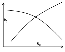
Figure 1. Intersection of singularity curves corresponding to two disconnected singular leaves.

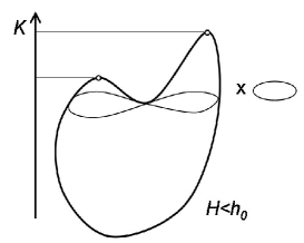
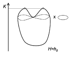
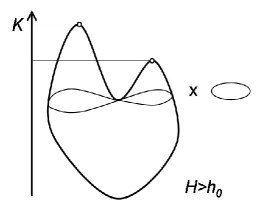
Figure 2. Isoenergy surfaces for different values of $H$ corresponding to the bifurcation diagram of Figure 1.

Thus, we need to refine the definition of $\Sigma_{c}$ so as to exclude such trivial cases from our consideration.

Consider a leaf $\mathcal{L}$ of the Liouville foliation. An open set $V$ which is invariant under the action $\Phi$ and contains $\mathcal{L}$ will be called an extended neighborhood of $\mathcal{L}$. For such a set $V$, denote by $\Sigma(V)$ the set of images of critical points of the momentum map restriction to $V$. We call $\Sigma(V)$ the local bifurcation set of $V$. As in the global case, $\Sigma(V)$ may itself have singularities, e.g. folds, common endpoints of curves, intersections or isolated points.

Denote by $\Sigma_{c}(V)\subset\Sigma_{c}$ the singularities of the local bifurcation set $\Sigma(V)$ as defined above. Clearly, for sufficiently thin extended neighborhoods, $\Sigma_{c}(V)$ is independent of $V$, so we may define a local critical point $\Sigma_{c}(\mathcal{L})=\Sigma_{c}(V)$. Notice that $\Sigma_{c}(\mathcal{L})$ is either empty or equal to $\{\mu(\mathcal{L})\}$.

We now introduce the essential critical set as the union of all local critical points over all foliation leaves of $\mathcal{M}$:

$$\Sigma_{c}^{ess}=\bigcup_{\mathcal{L}}\Sigma_{c}(\mathcal{L}).$$

Indeed, in the example shown on Figures 1 and 2, the level set $(h_{0},k_{0})$ consists of two isolated elliptic circles, and $\Sigma_{c}(\mathcal{L})=\emptyset$ for both of them. Thus $(h_{0},k_{0})$ does not belong to the essential critical set.

Clearly, non-degenerate singular leaves of rank $0$ and degenerate ones allowed by Assumption 5 will always produce essential singularities, see [38, 16]. However, this is not true for most non-degenerate singular leaves of rank $1$. Each non-degenerate one-dimensional orbit of $\Phi$ belongs to a smooth family of circles that is mapped by $\mu$ to a smooth curve of $\Sigma$. Stable singularities that may appear on such curves are folds and points of transversal intersection of two curves. We impose an additional stability condition: that all essential singularities appear on distinct isoenergy surfaces.

Assumption 6.

• Let $\mathcal{L}$, $\mathcal{L}^{\prime}$ be two distinct foliation leaves such that both have non-empty local critical points. Then $H(\mathcal{L})\neq H(\mathcal{L}^{\prime})$.

• Let $\mathcal{L}$ be a non-degenerate singular leaf of rank $1$ such that $\Sigma_{c}(\mathcal{L})\neq\emptyset$. Then, at the point $\mu(\mathcal{L})$ one of the following singularities occur:

  • a point of transversal intersection of two curves of $\Sigma$;

  • a quadratic fold of a curve of $\Sigma$.

The Singularities and Foliations Theorem is formulated for systems that satisfy Assumptions 1–6 and these include many natural mechanical systems (see Section 5).

3. The Singularities and Foliations Theorem

The main result of this paper is the formulation of the following theorem and its constructive proof. The main part of the proof is based on statements appearing in the next section and the appendices.

We say that isoenergy surfaces are Liouville equivalent if they are topologically conjugate and the homeomorphism preserves their Liouville foliations [12, 13, 14].

Singularities and Foliations Theorem.  Consider the $2$ degrees of freedom integrable Hamiltonian system $(\mathcal{M},\omega,H)$ satisfying Assumptions 1–6. Then, a change of the Liouville equivalence class of the isoenergy surfaces occurs at the energy level $H=h_{c}$ if and only if there exists a value $k_{c}$ such that $(h_{c},k_{c})\in\Sigma_{c}^{ess}$. Furthermore, there is a finite number of types of such possible changes. All of them are listed in Proposition 1, Proposition 2, Corollary 5, Corollary 8, and represented by the Fomenko graphs of Figures 3–8 and 10–19.

Proof.

$\Longrightarrow$ See Proposition 4.3 in [10]; We repeat here the proof for completeness. We prove this first part by contradiction. Assume that the isoenergy surfaces at $H=h_{1}$ and $H=h_{2}$ are not Liouville equivalent and that there is no $(h_{c},k_{c})\in\Sigma_{c}^{ess}$ with $h_{c}\in[h_{1},h_{2}].$ Assumptions 1–4 imply that with the exception of isolated values of $H$, the Liouville foliation of isoenergy surfaces may be completely described with the corresponding Fomenko invariants [14]. Vertices of the graph joined to the isoenergy surface $H=h$ correspond exactly to intersections of the line $H=h$ with $\Sigma$. Since we assumed there is no point of the set $\Sigma_{c}^{ess}$ between the lines $H=h_{1}$ and $H=h_{2}$, the Fomenko graphs, together with all their corresponding invariants, will change continuously between the values $h_{1}$ and $h_{2}$. Since the graph with all joined numerical invariants is given by a finite set of discrete parameters [14], it follows that all isoenergy surfaces $H=h$, where $h$ is between $h_{1}$ and $h_{2}$, have the same Fomenko invariants. Thus, the isoenergy surfaces $H=h_{1}$ and $H=h_{2}$ are Liouville equivalent, which concludes the proof.

$\Longleftarrow$ Take $(h_{c},k_{c})\in\Sigma_{c}^{ess}$. Then, there exists a singular leaf $\mathcal{L}$ such that $\mu(\mathcal{L})=(h_{c},k_{c})$ and $\Sigma_{c}(\mathcal{L})\neq\emptyset$. According to Assumption 5, there are three types of such singular leaves: non-degenerate leaves of rank $1$, degenerate leaves of rank $1$ and non-degenerate leaves of rank $0$.

If $\mathcal{L}$ is a non-degenerate leaf of rank $1$, the statement follows from Propositions 1 and 2. The changes in Liouville foliations are represented by Figures 3–8.

If $\mathcal{L}$ is a degenerate leaf admitting one of the allowed normal forms of Assumption 5, the statement follows from the works of [38, 35, 16] as summarized by Proposition 3. Possible changes in the Liouville foliations are described in Corollary 8 (see Appendix 2, Figures 17–19).

Finally, if $\mathcal{L}$ is a non-degenerate leaf of rank $0$, i.e. it contains a fixed point of the action $\Phi$, the statement follows from the works of [38, 10] as summarized by Proposition 4. The corresponding changes in the Liouville foliations are listed in Corollary 5 (see Appendix 2, Figures 10–16). ∎

Clearly, The Singularities and Foliations Theorem may be applied to the more restricted class of systems that do not have any smooth families of leaves of complexity $2$ (see Section 5). All possible essential singularities of such systems are included in the list of cases that appear in the theorem. Yet, for such simple systems, several types of bifurcations that are listed cannot be realized: the isolated non-orientable saddle-saddle fixed point, the symmetric degenerate circles undergoing a symmetric orientable saddle node bifurcation and the hyperbolic pitchfork bifurcation. Indeed, these are exactly the cases in which curves corresponding to complexity $2$ leaves appear near the critical set (see Figures 14, 15 and second lines of Figures 17 and 19).

4. Changes of Liouville Foliations near Essential Singularities

4.1. Behavior near Non-Degenerate Circles

Consider a non-degenerate leaf $\mathcal{L}$ of rank $1$, such that $\Sigma_{c}(\mathcal{L})\neq\emptyset$. By Assumption 6, the singularity of the bifurcation set appearing at $\mu(\mathcal{L})$ is a transversal intersection of two smooth curves or a quadratic fold. We analyze these two possibilities in Propositions 1 and 2 separately.

Proposition 1.

Consider a Hamiltonian system $(\mathcal{M},\omega,H)$ satisfying Assumptions 1–6. Suppose that a non-degenerate leaf $\mathcal{L}$ of rank $1$ is such that $\Sigma_{c}^{ess}(\mathcal{L})\neq\emptyset$ and $\mu(\mathcal{L})$ is a transversal intersection of two smooth curves from $\Sigma$. Then, for sufficiently small $|h-H(\mathcal{L})|$, the isoenergy surfaces for $h<H(\mathcal{L})$ and $h>H(\mathcal{L})$ are not Liouville equivalent. The Fomenko graphs that describe all the possible structures of the isoenergy surfaces near $\mathcal{L}$ are given by Figures 3 and 4.

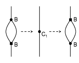
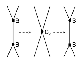
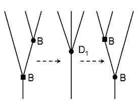
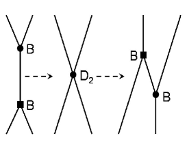
Figure 3. Global bifurcations in the orientable case. The four possible changes of the Liouville foliations near an intersection of two families of orientable hyperbolic circles that creates a non-degenerate singular leaf of rank $2$ (Proposition 1).

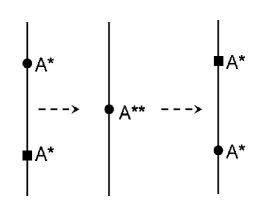
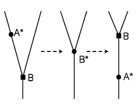
Figure 4. Global bifurcations in the non-orientable cases. Changes of the Liouville foliations near an intersection of two families of hyperbolic circles that creates a non-degenerate singular leaf of rank $2$. Left: both families of circles are non-orientable. Right: one orientable and one non-orientable families. (Proposition 1).

Proof.

Since, by Assumption 5, $\mathcal{L}$ may be of complexity of at most $2$, each of the curves $c_{1}$ and $c_{2}$ that intersect at $\mu(\mathcal{L})$ corresponds, away from $\mathcal{L}$, to a family of non-degenerate leaves of complexity $1$ and rank $1$ and the complexity of the leaf $\mathcal{L}$ is equal to $2$. The possible foliations of the isoenergy surface near such a leaf were completely classified by Fomenko (see [13]): there are exactly six kinds of such foliations, denoted by atoms $\mathbf{C}_{1}$, $\mathbf{C}_{2}$, $\mathbf{D}_{1}$, $\mathbf{D}_{2}$, $\mathbf{A}^{\ast\ast}$, $\mathbf{B}^{\ast}$.

Notice that the orientability of the circles along each of the curves $c_{1}$ and $c_{2}$ is fixed. Consider first the four atoms of complexity $2$ that have orientable circles: $\mathbf{C}_{1}$, $\mathbf{C}_{2}$, $\mathbf{D}_{1}$, $\mathbf{D}_{2}$. Each of these atoms dictates uniquely the form of the foliations in the nearby isoenergy surfaces as summarized by Figure 3.

Suppose first that the Fomenko atom corresponding to the isoenergy surface of $\gamma$ is $\mathbf{C}_{1}$. Because only one edge of the Fomenko graph joins the atom $\mathbf{C}_{1}$ from each side, it follows that there is exactly one Liouville torus projected to each point placed above or under both the curves $c_{1}$ and $c_{2}$. This means that two such tori are projected to points between the curves.

Now consider the case of atom $\mathbf{D}_{1}$. Then, three families of Liouville tori should appear above the two curves $c_{1}$ and $c_{2}$, and only one family appears for points below the two curves. The unique way to achieve this behavior is shown.

The remaining cases, of atoms $\mathbf{C}_{2}$ and $\mathbf{D}_{2}$ exhibit a similar behavior: both have two families of tori below and above the two curves $c_{1}$ and $c_{2}$. To distinguish between these two cases, we note that the singular level sets corresponding to the atoms $\mathbf{C}_{1}$ and $\mathbf{C}_{2}$ are isomorphic – both have two oriented singular periodic trajectories and four heteroclinic separatrices. Similarly, $\mathbf{D}_{1}$ and $\mathbf{D}_{2}$ are isomorphic: both have two homoclinic separatrices – one joined to each circle from $\mathcal{L}$, and two heteroclinic ones.

Suppose now that $\mathbf{C}_{2}$ is the atom joined to the isoenergy surface containing $\mathcal{L}$. Now, we will look for the Fomenko graphs corresponding to the submanifolds $K=\mathrm{const}$. The atom corresponding to $K=K(\mathcal{L})$ must be one with the singular level set isomorphic to $\mathbf{C}_{2}$, thus it is $\mathbf{C}_{1}$ or $\mathbf{C}_{2}$. If it is $\mathbf{C}_{2}$, we would have again two Liouville tori above any point between the curves $c_{1}$ and $c_{2}$. But, it is easy to see that this is not possible since the curves $c_{1}$, $c_{2}$ correspond to $\mathbf{B}$-atoms. So, the Fomenko atom for the submanifold $K=K(\mathcal{L})$ is $\mathbf{C}_{1}$ which was described above. Hence, there is exactly one family of Liouville tori between the curves $c_{1}$ and $c_{2}$. Finally, the case of atom $\mathbf{D}_{2}$ may be similarly analyzed. We conclude that the atom $\mathbf{D}_{1}$ is joined to the submanifold $K=K(\gamma)$, and the Fomenko graphs describing the extended neighborhood $V$ are indeed uniquely constructed and can be seen in Figure 3.

Cases when at least one of the curves $c_{1}$, $c_{2}$ corresponds to a family of nonorientable circles are resolved directly from the structure of the corresponding Fomenko atoms: $\mathbf{A}^{\ast\ast}$ and $\mathbf{B}^{\ast}$. The graphs are shown on Figure 4.

Finally, let us remark that the graphs corresponding to the cases when the atoms $\mathbf{C}_{1}$, $\mathbf{C}_{2}$, $\mathbf{A^{**}}$ appear, are isomorphic for $h<H(\mathcal{L})$ and $h>H(\mathcal{L})$. Nevertheless, since the $r$-marks corresponding to the upper and lower edges will be changed, the Liouville foliations are not equivalent. ∎

We now list the Liouville foliation structure of the isoenergy surfaces near the circles of fixed points that appear persistently when a curve belonging to $\Sigma$ has a fold.

Proposition 2.

Consider a Hamiltonian system $(\mathcal{M},\omega,H)$ satisfying Assumptions 1-6. Suppose that a non-degenerate leaf $\mathcal{L}$ of rank $1$ is such that $\mu(\mathcal{L})$ is a fold of a smooth curve from $\Sigma$. Then $\Sigma_{c}^{ess}(\mathcal{L})\neq\emptyset$. Moreover, for sufficiently small $|h-H(\mathcal{L})|$, the isoenergy surfaces for $h<H(\mathcal{L})$ and $h>H(\mathcal{L})$ are not Liouville equivalent. If $\mathcal{L}$ is of complexity $1$, then the possible foliations of isoenergy surfaces near the leaf are completely described by Figures 5, 6, and 7. For the leaf of complexity $2$, the foliations are shown on Figure 8.

Proof.

Consider a sufficiently small extended neighborhood $V$ of $\mathcal{L}$. Clearly, for sufficiently small $\varepsilon$, only one submanifold $V\cap{H}^{-1}(H(\mathcal{L})+\varepsilon)$, $V\cap{H}^{-1}(H(\mathcal{L})-\varepsilon)$ contains singular leaves. Thus, the corresponding isoenergy surfaces are not Liouville equivalent.

Now, suppose that $\mathcal{L}$ contains a unique circle $\gamma$. Denote by $c$ the curve of $\Sigma$ with the fold $\mu(\gamma)$. $c$ divides a small convex neighborhood $N$ of $\mu(\gamma)$ in $\mathbf{R}^{2}$ into a convex and concave part, see Figure 5.

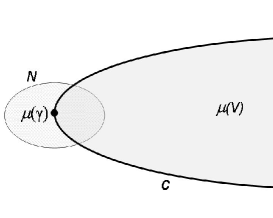
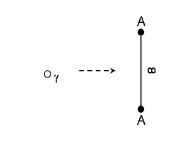
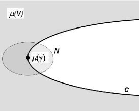
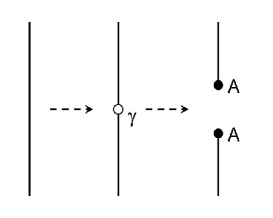
Figure 5. The two cases of an Elliptic fold; Left: the bifurcation sets — the solid curve corresponds to a family of elliptic circles and the allowed region of motion is shaded. Right: the changes in the Liouville foliations as described by the Fomenko graphs (Proposition 2).

Suppose first that $\gamma$ is a normally elliptic circle, i.e. that the curve $c$ corresponds to a family of Fomenko $\mathbf{A}$-atoms. If $\mu(V)$ has no intersection with the concave part of $N$ (first line of Figure 5), the energy surfaces near $\gamma$ are locally diffeomorphic to $\mathbf{S}^{2}\times\mathbf{S}^{1}$. On the other hand, if $\mu(V)$ has no intersection with the convex part of $N$ (second line of Figure 5), the isoenergy surfaces near $\gamma$ are locally diffeomorphic to $(0,1)\times\mathbf{T}^{2}$ for $H<H(\gamma)$ and to a disjoint union of two solid tori for $H>H(\gamma)$, or vice versa.

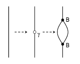
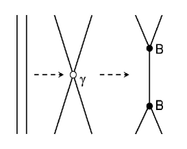
Figure 6. An orientable hyperbolic fold; The two possible changes in the Liouville foliations near a fold of a curve in the bifurcation set when the curve corresponds to a family of hyperbolic orientable circles (Proposition 2).

If $\gamma$ is normally hyperbolic and orientable, there may be one or two Liouville tori in $V$ over each point in the convex part of $N$. The corresponding Fomenko graphs are shown on Figure 6.

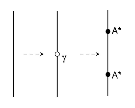
Figure 7. A non-orientable hyperbolic fold; The change in the Liouville foliations near a fold of a curve in the bifurcation set when the curve corresponds to a family of hyperbolic non-orientable circles (Proposition 2).

If $\gamma$ is non-orientable normally hyperbolic circle, the corresponding Fomenko graphs are shown on Figure 7.

Finally, for $\mathcal{L}$ of complexity $2$, the Fomenko graphs are shown on Figure 8.∎

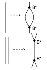
Figure 8. A fold of complexity $2$; The possible changes in the Liouville foliations near a fold of a curve in the bifurcation set when the curve corresponds to a family of non-degenerate complexity $2$ leaves (Proposition 2).

4.2. Behavior near Parabolic Circles

The behavior of the level sets near degenerate singular leaves that are allowed by Assumption 5, namely near parabolic circles, was essentially described in the generic, non-symmetric case in [38] and [35], and by [16] under some additional symmetry assumptions. From these works we can immediately conclude:

Proposition 3.

Consider a Hamiltonian system $(\mathcal{M},\omega,H)$ satisfying Assumptions 1–5, and its degenerate leaf $\mathcal{L}$ of rank $1$. Then $\mu(\mathcal{L})\in\Sigma_{c}^{ess}$. Moreover, for sufficiently small $|h-H(\mathcal{L})|$, the isoenergy surfaces for $h<H(\mathcal{L})$ and $h>H(\mathcal{L})$ are not Liouville equivalent. The bifurcation sets and foliations of isoenergy surfaces near $\mathcal{L}$ are represented by Figures 17, 18, and 19 in Appendix 2.

Proof.

The local bifurcation sets near parabolic circles satisfying Assumption 5 and some more general cases, are constructed in [16], see also [38] and [35]. The bifurcation sets are represented by Figures 17–19 in Appendix 2. Clearly, in all cases several curves meet at $\mu(\mathcal{L})$ so it is an essential singularity of the bifurcation set.

In addition, since the number of singular leaves on the isoenergy surfaces near $\mathcal{L}$ is not the same for $h<H(\mathcal{L})$ and $h>H(\mathcal{L})$, they cannot be Liouville equivalent.

The corresponding Fomenko graphs are represented by Figures 17–19 in Appendix 2 — these graphs are easily inferred from the circular graphs of [16]. Notice that curves of leafs of complexity 2 are created in some of the symmetric cases. ∎

4.3. Behavior near Fixed Points

The book of Lerman and Umanskii [38] provides the analysis and complete description of the structure of the level sets near non-degenerate fixed points, under somewhat weaker conditions than Assumptions 1–5. In Appendix 2, we succinctly summarize this description of the foliation near the fixed points in Corollary 5 by using the bifurcation diagrams and Fomenko graphs (see also [10, 46] for a very similar description). We remark that although the resulting graphs are simple, the topology associated with each of these cases may be highly non-trivial as is described in details in [38]. The following proposition is needed to prove our main singularity and bifurcation theorem.

Proposition 4.

Let $(\mathcal{M},\omega,H)$ be a Hamiltonian system satisfying Assumptions 1-5 and $p\in\mathcal{M}$ a fixed point of the Poisson action. Then $\mu(p)\in\Sigma_{c}^{ess}$.

Moreover, for sufficiently small $|h-H(p)|$, the isoenergy surfaces for $h<H(p)$ and $h>H(p)$ are not Liouville equivalent. The bifurcation sets and the possible structures of the isoenergy surfaces near $p$ are shown on Figures 10–16 in Appendix 2.

Proof.

The local bifurcation sets near different types of fixed points are constructed in [38]. Here, they are represented by Figures 10–16 in Appendix 2, and it is clear that in each case $\mu(p)$ is an essential singularity of the bifurcation set as several curves meet at $\mu(p)$.

Relying on [38] and [10], we list in Appendix 2 the marked Fomenko graphs for the isoenergy surfaces close to $p$ for all the non-degenerate cases. When those graphs are different for $h<H(p)$ and $h>H(p)$, the proposition immediately follows. However, in the few cases that are listed below, the corresponding graphs are the same, so additional arguments are needed.

The first case appears when $p$ is of the center-center type and $\mu(p)$ is not a local extremum point for the Hamiltonian $H$ (second line of Figure 10). Yet, the $r$-marks corresponding to the edges of the Fomenko graphs represented by Figure 10 are different. Thus, the isoenergy surfaces are not Liouville equivalent.

The second case is when $p$ is of the saddle-saddle type, with all four one-dimensional orbits of action in its leaf being orientable, when all near-by isoenergy surfaces have the same number of singular leaves, as shown on the second line of Figure 12. However, similarly as before the $r$-marks corresponding to the upper and lower edges of Fomenko graphs are not the same on for $h<H(p)$ and $h>H(p)$.

The last case is when $p$ is of focus-focus type, as shown by Figure 16. Then the leaf of $p$ is the only singular leaf in a sufficiently small extended neighborhood. As it is noted in Remark 7 of Appendix 2, the $r$-marks on the corresponding edges of Fomenko graphs are changed, which concludes the proof. ∎

5. Examples

5.1. Examples of Systems with only Isolated Leaves of Complexity $2$

Integrable Hamiltonian systems of the form:

$$H(x,y,I,\theta)=H_{0}(x,y,I)\quad(x,y,I,\theta)\in\mathbf{R}^{3}\times\mathbf{S}^{1}$$

with non-degenerate dependence on $(x,y,I)$ (and in particular no $\mathbf{Z}_{2}$–symmetry in the $(x,y)$–plane) satisfy Assumptions 1-6. For example, for an open dense set of $\varepsilon,\omega>0$, the following system

(1) $$H(x,y,I,\theta;\varepsilon,\omega)=\frac{y^{2}}{2}+I\,\frac{x^{2}}{2}+\varepsilon x^{3}+\frac{x^{4}}{4}+(I+\omega)^{2},\quad(x,y,I,\theta)\in\mathbf{R}^{3}\times\mathbf{S}^{1}$$

satisfies these conditions: it has compact level sets and compact isoenergy surfaces and is non-degenerate. Since it has no fixed points, and the only rank $1$ orbits correspond to $(x(I),y(I))$ values at which $\nabla_{(x,y)}H_{0}=0$, Assumptions 5–6 may be easily verified.

To produce non-degenerate fixed points in the above construction we may take:

$$I=u^{2}+v^{2}-c$$

where $c\neq 0$ is yet another non-degeneracy parameter, so that equation (1) can now have center-center or center-saddle non-degenerate fixed points, depending on the value of $c$. Then the system is defined for $I\geq-c$.

The Truncated Forced Nonlinear Schroedinger Equation

The truncated forced nonlinear Schroedinger equation corresponds to a two-mode Galerkin truncation of the corresponding forced integrable partial differential equation, see [8, 6, 5, 7, 19, 55] and references therein. The corresponding truncated Hamiltonian is:

$$H(c,c^{\ast},b,b^{\ast};\varepsilon)=H_{0}(c,c^{\ast},b,b^{\ast})+\varepsilon H_{1}(c,c^{\ast},b,b^{\ast}),$$

with the Poisson brackets $\{f,g\}=-2i\left(\left\langle\frac{\partial}{\partial c},\frac{\partial}{\partial c^{\ast}}\right\rangle+\left\langle\frac{\partial}{\partial b},\frac{\partial}{\partial b^{\ast}}\right\rangle\right)$, where

$$H_{0} =\frac{1}{8}|c|^{4}+\frac{1}{2}|b|^{2}|c|^{2}+\frac{3}{16}|b|^{4}-\frac{1}{2}(\Omega^{2}+k^{2})|b|^{2}-\frac{\Omega^{2}}{2}|c|^{2}+\frac{1}{8}(b^{2}c^{\ast 2}+b^{\ast 2}c^{2})$$

$$H_{1} =\frac{-i}{\sqrt{2}}(c-c^{\ast}).$$

At $\varepsilon=0$ the Hamiltonian flow possesses an additional integral of motion:

$$I=\frac{1}{2}(|c|^{2}+|b|^{2})$$

and is thus integrable, see [8, 6, 5, 7, 19]. Using this integral of motion one may bring this system to the form (1), and thus the bifurcation diagrams and the corresponding Fomenko graphs may be constructed for any concrete numerical values of the parameters (see Figures 1 and 2 from [55]). A representative sequence of graphs from [55] (here we add the labels of the Fomenko atoms and do not provide a different symbol to each of the four different families of circles that appear in this problem), is shown in Figure 9.

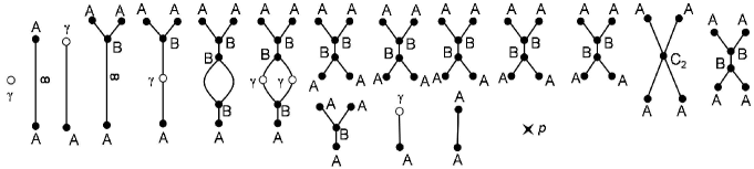
Figure 9. Fomenko graphs for the truncated NLS.

We see that in this example, the following bifurcations appear:

• Folds of elliptic and orientable hyperbolic circles (Proposition 2).

• Center-Center point (Corollary 5).

• Symmetric orientable parabolic circles with the elliptic pitchfork normal form $hx^{2}+x^{4}+y^{2}$(Corollary 8).

• Global bifurcation of orientable circles creating a $\mathbf{C}_{2}$-atom (Proposition 1).

We see that rank-1 orbits of complexity 2 appear only at isolated values (at an orientable global bifurcation).

5.2. Examples of Integrable Rigid Body Motion

The topological structure of integrable cases of the rigid body motion had been extensively studied and analyzed by the Fomenko school and others [16, 52], producing examples of many of the bifurcations that are listed in Corollary 5 and Corollary 8.

For example, the topology of the Kovalevskaya top dynamics is studied in detail in [16]. In the bifurcation diagram, there appears a line corresponding to a non-orientable family of circles ($\mathbf{A}^{*}$–atoms). It follows that for a perturbation which is resonant with one circle of this non-orientable family — namely, for the appropriate choice of integrals — we will have a bifurcation diagram corresponding to a fold of a non-orientable family of circles, as in Proposition 2. We also note that in this case there is a saddle-saddle fixed point with $2$ non-orientable orbits in its leaf, which creates in the bifurcation set a curve along which the complexity $2$ atom $\mathbf{C}_{2}$ appears.

6. Conclusions

The main result of this paper is the Singularities and Foliations Theorem, which, together with Propositions 1, 2 and Corollaries 5, 8 from Appendix 2 gives a classification of the changes in the isoenergy surfaces for a class of two degrees of freedom Hamiltonian systems.

Surprisingly, the study of the level sets structure near singular circles had lead to the discovery of several new phenomena that may be of future interest in the near-integrable context; first, the persistent appearance of folds of curves in the energy-momentum bifurcation diagrams and its implications had been fully analyzed. Notably, the appearance of a circle of hyperbolic fixed points with non-orientable separatrices (type $\mathbf{A}^{\ast}$) had emerged as a ”generic” scenario which had not been studied yet; under small perturbations we expect to obtain various multi-pulse orbits to some resonance zone which will replace the circle of fixed points. While the tools developed by Haller [34, 32] and Kovačič [36] to study the orientable case should apply, the nature of the chaotic set may be quite different. Second, the complete listing of the structure of the isoenergy surfaces near all non-degenerate global bifurcations may lead to a systematic study of the emerging chaotic sets of the various cases under small perturbations. Let us note that such a listing follows from [13], but is usually presented in the different context of the completely integrable dynamics.

Beyond the classification result, the present paper together with [40, 41, 42, 55] supply a tool for studying near-integrable systems; In [55] we proposed that the bifurcations of the level sets in such systems may be studied by a three level hierarchal structure. The first level corresponds to finding singular level sets on any given energy surface – namely of finding the bifurcation set and the structure of the corresponding isoenergy surfaces as described by the Fomenko graphs. The second level consists of finding the singularities of the bifurcation set of the system, and finding which ones are essential – namely identifying the essential critical set – the set of all values of the energy where the foliation of the isoenergy surfaces changes. The third level consists of investigating singularities in the critical set as parameters are varied.

Combining Fomenko school works and Lerman and Umanskii works leads to a complete classification of the first level for the non-degenerate systems considered here. We supply a complete classification of the second level in this hierarchy for the systems satisfying Assumptions 1–6. A classification of the third level and of more complex systems that may arise under symmetric settings is yet to be constructed.

Having this classification of the second level means that given the structure of an isoenergy surface at some fixed energy, we can now develop the global structure of all isoenergy surfaces by continuation, using our classification of the energy surface structure near the critical set. Namely, a topological continuation scheme may be implemented , and it will be interesting to relate it to [23] where a continuation scheme for finding the action angle coordinates is found.

Acknowledgements

We thank Prof. L. Lerman, A. Bolsinov, V. Dragović, and H. Hanssman for important comments and discussion. The research is supported by the Minerva foundation, by the Russian-Israeli joint grant and by the Israel Science Foundation (grant no 273/07). One of the authors (M.R.) is supported by the Serbian Ministry of Science and Technology, Project no. 144014: Geometry and Topology of Manifolds and Integrable Dynamical Systems.

Appendix 1: Topological Classification of Isoenergy Surfaces

In this section, we describe the representation of isoenergy surfaces and some of their topological invariants by Fomenko graphs.

Consider a Hamiltonian system defined on the manifold $\mathcal{M}$, satisfying Assumptions 1–4.

Two isoenergy surfaces $\mathcal{Q}$ and $\mathcal{Q}^{\prime}$ are Liouville equivalent if there exists a homeomorphism between them preserving their Liouville foliations.

The set of topological invariants that describe completely isoenergy manifolds containing regular and non-degenerate leaves of rank $1$, up to their Liouville equivalence, consists of:

• The oriented graph $G$, whose vertices correspond to the singular connected components of the level sets of $K$, and edges to one-parameter families of Liouville tori;

• The collection of Fomenko atoms, such that each atom marks exactly one vertex of the graph $G$;

• The collection of pairs of numbers $(r_{i},\varepsilon_{i})$, with $r_{i}\in([0,1)\cap\mathbf{Q})\cup\{\infty\}$, $\varepsilon_{i}\in\{-1,1\}$, $1\leq i\leq n$. Here, $n$ is the number of edges of the graph $G$ and each pair $(r_{i},\varepsilon_{i})$ marks an edge of the graph;

• The collection of integers $n_{1},n_{2},\dots,n_{s}$. The numbers $n_{k}$ correspond to certain connected components of the subgraph $G^{0}$ of $G$. $G^{0}$ consists of all vertices of $G$ and the edges marked with $r_{i}=\infty$. The connected components marked with integers $n_{k}$ are those that do not contain a vertex corresponding to an isolated critical circle (an $\mathbf{A}$ atom) on the manifold $\mathcal{Q}$.

Let us clarify the meaning of some of these invariants.

First, we are going to describe the construction of the graph $G$ from the manifold $\mathcal{Q}$. Each singular leaf of the Liouville foliation corresponds to exactly one vertex of the graph. If we cut $\mathcal{Q}$ along such leaves, the manifold will fall apart into connected sets, each one consisting of one-parameter family of Liouville tori. Each of these families is represented by an edge of the graph $G$. The vertex of $G$ which corresponds to a singular leaf $\mathcal{L}$ is incident to the edge corresponding to the family $\mathcal{T}$ of tori if and only if $\partial\mathcal{T}\cap\mathcal{L}$ is non empty.

Note that $\partial\mathcal{T}$ has two connected components, each corresponding to a singular leaf. If the two singular leaves coincide, then the edge creates a loop connecting one vertex to itself.

Now, when the graph is constructed, one need to add the orientation to each edge. This may be done arbitrarily, but, once determined, the orientation must stay fixed because the values of numerical Fomenko invariants depend on it.

The Fomenko atom which corresponds to a singular leaf $\mathcal{L}$ of a singular level set is determined by the topological type of the set $\mathcal{L}_{\varepsilon}$. The set $\mathcal{L}_{\varepsilon}\supset{\mathcal{L}}$ is the connected component of $\{\ p\in\mathcal{Q}\ |\ c-\varepsilon<K(p)<c+\varepsilon\ \}$, where $c=K(\mathcal{L})$, and $\varepsilon>0$ is such that $c$ is the only critical value of the function $K$ on $\mathcal{Q}$ in interval $(c-\varepsilon,c+\varepsilon)$.

Let $\mathcal{L}_{\varepsilon}^{+}=\{\ p\in\mathcal{L}_{\varepsilon}\ |\ K(p)>c\ \}$, $\mathcal{L}_{\varepsilon}^{-}=\{\ p\in\mathcal{L}_{\varepsilon}\ |\ K(p)<c\ \}$. Each of the sets $\mathcal{L}_{\varepsilon}^{+}$, $\mathcal{L}_{\varepsilon}^{-}$ is a union of several connected components, each component being a one-parameter family of Liouville tori. Each of these families corresponds to the beginning of an edge of the graph $G$ incident to the vertex corresponding to $\mathcal{L}$.

Let us say a few words on the topological structure of the set $\mathcal{L}$. This set consists of at least one fixed point or closed one-dimensional orbit of the Poisson action $\Phi$ on $\mathcal{M}$ and several (possibly none) two-dimensional orbits of the action. The set of all zero-dimensional and one-dimensional orbits in $\mathcal{L}$ is called the garland (see [38]) while two-dimensional orbits are called separatrices.

The trajectories on each of these two-dimensional separatrices is homoclinically or heteroclinically tending to the lower-dimensional orbits. The Liouville tori of each of the families in $\mathcal{L}_{\varepsilon}\setminus\mathcal{L}=\mathcal{L}_{\varepsilon}^{+}\cup\mathcal{L}_{\varepsilon}^{-}$ tend, as the integral $K$ approaches $c$, to a closure of a subset of the separatrix set.

Fomenko Atoms of Complexity 1 and 2

Fomenko and his school completely described and classified non-degenerate leaves of rank $1$.

If $\mathcal{L}$ is not an isolated critical circle, then a sufficiently small neighborhood of each $1$-dimensional orbit in $\mathcal{L}$ is isomorphic to either two cylinders intersecting along the base circle, and then the orbit is orientable, or to two Moebius bands intersecting each other along the joint base circle, then the $1$-dimensional orbit is non-orientable.

The number of closed one-dimensional orbits in $\mathcal{L}$ is called the complexity of the corresponding atom.

There are exactly three Fomenko atoms of complexity $1$.

The atom $\mathbf{A}$.

This atom corresponds to a normally elliptic singular circle, which is isolated on the isoenergy surface $\mathcal{Q}$. A small neighborhood of such a circle in $\mathcal{Q}$ is diffeomorphic to a solid torus. One of the sets $\mathcal{L}_{\varepsilon}^{+}$, $\mathcal{L}_{\varepsilon}^{-}$ is empty, the other one is connected. Thus only one edge of the graph $G$ is incident with the vertex marked with the letter atom $\mathbf{A}$.

The atom $\mathbf{B}$.

In this case, $\mathcal{L}$ consists of one orientable normally hyperbolic circle and two $2$-dimensional separatrices – it is diffeomorphic to a direct product of the circle $\mathbf{S}^{1}$ and the plane curve given by the equation $y^{2}=x^{2}-x^{4}$. Because of its shape, we will refer to this curve as the ‘figure eight’. The set $\mathcal{L}_{\varepsilon}\setminus\mathcal{L}$ has $3$ connected components, two of them being placed in $\mathcal{L}_{\varepsilon}^{+}$ and one in $\mathcal{L}_{\varepsilon}^{-}$, or vice versa. Let us fix that two of them are in $\mathcal{L}_{\varepsilon}^{+}$. Each of these two families of Liouville tori limits as $K$ approaches $c$ to only one of the separatrices. The tori in $\mathcal{L}_{\varepsilon}^{-}$ tend to the union of the separatrices.

The atom $\mathbf{A}^{*}$.

$\mathcal{L}$ consists of one non-orientable hyperbolic circle and one $2$-dimensional separatrix. It is homeomorphic to the smooth bundle over $\mathbf{S}^{1}$ with the ‘figure eight’ as fiber and the structural group consisting of the identity mapping and the central symmetry of the ‘figure eight’. Both $\mathcal{L}_{\varepsilon}^{+}$ and $\mathcal{L}_{\varepsilon}^{-}$ are $1$-parameter families of Liouville tori, one limiting to the separatrix from outside the ‘figure eight’ and the other from the interior part of the ‘figure eight’.

The atoms of complexity $2$ appear in the non-degenerate integrable two degrees of freedom systems considered here on isoenergy surfaces close to fixed points of the system, and, for isolated values of the energy $H$, at level sets corresponding to global bifurcations of the system. Fomenko showed that there are exactly six different atoms of complexity $2$, and these are described next. It is instructive to use the Fomenko graphs depicted in the figures of propositions 1 and 2 to understand the structure of the level sets near these complexity 2 atoms.

The atom $\mathbf{C}_{1}$.

$\mathcal{L}$ consists of two orientable circles $\gamma_{1}$, $\gamma_{2}$ and four heteroclinic $2$-dimensional separatrices $\mathcal{S}_{1}$, $\mathcal{S}_{2}$, $\mathcal{S}_{3}$, $\mathcal{S}_{4}$. Trajectories on $\mathcal{S}_{1}$, $\mathcal{S}_{3}$ are approaching $\gamma_{1}$ as time tend to $\infty$, and $\gamma_{2}$ as time tend to $-\infty$, while those placed on $\mathcal{S}_{2}$, $\mathcal{S}_{4}$ approach $\gamma_{2}$ as time tend to $\infty$, and $\gamma_{1}$ as time tend to $-\infty$. Each of the sets $\mathcal{L}_{\varepsilon}^{+}$, $\mathcal{L}_{\varepsilon}^{-}$ is connected and contains only one family of Liouville tori. Both families of tori deform to the whole separatrix set, as the value of $K$ approaches $c$.

The atom $\mathbf{C}_{2}$.

The level set $\mathcal{L}$ is the same as in the atom $\mathbf{C}_{1}$. Each of the sets $\mathcal{L}_{\varepsilon}^{+}$, $\mathcal{L}_{\varepsilon}^{-}$ contains two families of Liouville tori. As $K$ approaches to $c$, the tori from one family in $\mathcal{L}_{\varepsilon}^{-}$ deform to $\mathcal{S}_{1}\cup\mathcal{S}_{2}$, and from the other one to $\mathcal{S}_{3}\cup\mathcal{S}_{4}$. The tori from one family in $\mathcal{L}_{\varepsilon}^{+}$ is deformed to $\mathcal{S}_{1}\cup\mathcal{S}_{4}$, and from the other to $\mathcal{S}_{2}\cup\mathcal{S}_{3}$.

The atom $\mathbf{D}_{1}$.

$\mathcal{L}$ consists of two orientable circles $\gamma_{1}$, $\gamma_{2}$ and four $2$-dimensional separatrices $\mathcal{S}_{1}$, $\mathcal{S}_{2}$, $\mathcal{S}_{3}$, $\mathcal{S}_{4}$. Trajectories of $\mathcal{S}_{1}$, $\mathcal{S}_{2}$ homoclinically tend to $\gamma_{1}$, $\gamma_{2}$ respectively. Trajectories on $\mathcal{S}_{3}$ are approaching $\gamma_{1}$ as time tend to $\infty$, and $\gamma_{2}$ as time tend to $-\infty$, while those placed on $\mathcal{S}_{4}$, approach $\gamma_{2}$ as time tend to $\infty$, and $\gamma_{1}$ as time tend to $-\infty$. One of the sets $\mathcal{L}_{\varepsilon}^{+}$, $\mathcal{L}_{\varepsilon}^{-}$ contains three, and the other one family of Liouville tori. Lets say that $\mathcal{L}_{\varepsilon}^{+}$ contains three families. As $K$ approaches to $c$, these families deform to $\mathcal{S}_{1}$, $\mathcal{S}_{2}$ and $\mathcal{S}_{3}\cap\mathcal{S}_{4}$ respectively, while the family contained in $\mathcal{L}_{\varepsilon}^{-}$ deform to the whole separatrix set.

The atom $\mathbf{D}_{2}$.

The level set $\mathcal{L}$ is the same as in the atom $\mathbf{D}_{1}$. Each of the sets $\mathcal{L}_{\varepsilon}^{+}$, $\mathcal{L}_{\varepsilon}^{-}$ contains two families of Liouville tori. As $K$ approaches to $c$, the tori from one family in $\mathcal{L}_{\varepsilon}^{-}$ deform to $\mathcal{S}_{1}$, and from the other one to $\mathcal{S}_{2}\cup\mathcal{S}_{3}\cup\mathcal{S}_{4}$. The tori from one family in $\mathcal{L}_{\varepsilon}^{+}$ is deformed to $\mathcal{S}_{2}$, and from the other to $\mathcal{S}_{1}\cup\mathcal{S}_{3}\cup\mathcal{S}_{4}$.

The atom $\mathbf{B}^{*}$.

$\mathcal{L}$ consists of the orientable circle $\gamma_{1}$, the non-orientable circle $\gamma_{2}$ and three separatrices $\mathcal{S}_{1}$, $\mathcal{S}_{2}$, $\mathcal{S}_{3}$. Trajectories on $\mathcal{S}_{1}$ homoclinically tend to $\gamma_{1}$. Trajectories on $\mathcal{S}_{2}$ are approaching $\gamma_{1}$ as time tend to $\infty$, and $\gamma_{2}$ as time tend to $-\infty$, while those placed on $\mathcal{S}_{3}$, approach $\gamma_{2}$ as time tend to $\infty$, and $\gamma_{1}$ as time tend to $-\infty$. One of the sets $\mathcal{L}_{\varepsilon}^{+}$, $\mathcal{L}_{\varepsilon}^{-}$ contains two, and the other one family of Liouville tori. Lets say that $\mathcal{L}_{\varepsilon}^{+}$ contains two families. Then tori from these two families deform to $\mathcal{S}_{1}$ and $\mathcal{S}_{2}\cup\mathcal{S}_{3}$ respectively, as $K$ approaches to $c$. The tori from the $\mathcal{L}_{\varepsilon}^{-}$ deform to the union of the whole separatrix set.

The atom $\mathbf{A}^{**}$.

$\mathcal{L}$ consists of two non-orientable circles $\gamma_{1}$, $\gamma_{2}$ and two separatrices $\mathcal{S}_{1}$, $\mathcal{S}_{2}$. Trajectories on $\mathcal{S}_{1}$ are approaching $\gamma_{1}$ as time tend to $\infty$, and $\gamma_{2}$ as time tend to $-\infty$, while those placed on $\mathcal{S}_{2}$, approach $\gamma_{2}$ as time tend to $\infty$, and $\gamma_{1}$ as time tend to $-\infty$. Each of the sets $\mathcal{L}_{\varepsilon}^{+}$, $\mathcal{L}_{\varepsilon}^{-}$ consists of one family of Liouville tori. As $K$ approaches to $c$, the tori from both families deform to the whole separatrix set.

This concludes the complete list of all atoms of complexities $1$ and $2$, i.e. all the possible singular level sets which involve one or two circles and their separatrices. The appearance of higher complexities violates our non-degeneracy assumptions. These are expected to appear when additional symmetries, additional parameters, or higher dimensional systems are considered.

Numerical Fomenko Invariants

The meaning of the numerical invariant $r_{i}$ is roughly explained next.

Each edge of the Fomenko graph corresponds to a one-parameter family of Liouville tori. Let us cut each of these families along one Liouville torus. The manifold $\mathcal{Q}$ will disintegrate into pieces, each corresponding to the singular level set, i.e. to a part of the Fomenko graph containing only one vertex and the initial segments of the edges incident to this vertex. To reconstruct $\mathcal{Q}$ from these pieces, we need to identify the corresponding boundary tori. This can be done in different ways, implicating different differential-topological structure of the obtained manifold, and the number $r_{i}$ contains the information on the rule of the gluing on each edge.

Two important values of $r_{i}$ are $0$ and $\infty$. Consider one edge of the graph and the corresponding smooth one-parameter family $\mathcal{L}$ of Liouville tori. After cutting, the family falls apart into two families of tori diffeomorphic to the product $(0,1]\times\mathbf{T}^{2}\simeq(0,1]\times\mathbf{S}^{1}\times\mathbf{S}^{1}$. Such a family can be trivially embedded to the full torus $\mathbf{D}^{2}\times\mathbf{S}^{1}$ by the mapping $\phi\times\mathrm{id}_{\mathbf{S}^{1}}$, with

$$\phi\ :\ (0,1]\times\mathbf{S}^{1}\ \rightarrow\ \mathbf{D}^{2},\quad\phi(r,\alpha)=(r\cos\alpha,r\sin\alpha),$$

where we take $\mathbf{S}^{1}=\mathbf{R}/2\pi\mathbf{Z}$, $\mathbf{D}^{2}=\{\ (x,y)\in\mathbf{R}^{2}\ |\ x^{2}+y^{2}\leq 1\ \}$.

Now, via the gluing, the family $\mathcal{L}$ will be embedded to a the three-dimensional manifold $\mathcal{T}$ obtained from two solid tori by identifying their boundaries. The value $r_{i}=0$ corresponds to the case when the central circles of the two solid tori are linked in $\mathcal{T}$ with the linking coefficient $1$. $\mathcal{T}$ is then diffeomorphic to the sphere $\mathbf{S}^{3}$. The value $r_{i}=\infty$ corresponds to the case when the central circles are not linked in $\mathcal{T}$. In this case, $\mathcal{T}\simeq\mathbf{S}^{2}\times\mathbf{S}^{1}$.

For more detailed description and precise methods for determining the invariant $r_{i}$, see [13, 47].

The invariants $\varepsilon_{i}$, $n_{k}$ are not important for our exposition; their detailed description with the examples can be found in [13].

Appendix 2: Isonergy Surfaces near Isolated Fixed Points and Parabolic Circles

Here we provide for completeness the description of isoenergy surfaces for cases that were fully analyzed previously: the behavior near isolated fixed points, which is essentially a concise summary of Lerman and Umanskii [38] results using Fomenko graphs [10] and the behavior near certain parabolic circles which follows from [16].

The bifurcation diagrams that we draw for all these cases correspond to a slight modification of the standard energy-momentum diagrams and include the following elements:

• Solid curves correspond to families of normally elliptic circles, i.e. to Fomenko $\mathbf{A}$-atoms.

• Dashed curves correspond to families of normally hyperbolic circles.

• Double lines are used to indicate that two families of circles appear on the same curve in the bifurcation set.

• Grey area indicates the local region of allowed motion.

The topology of the level sets and of the extended neighborhoods of non-degenerate simple fixed points is described in detail in [38]. In the following corollary, we give a concise summary of these results with an emphasize on listing the possible changes in the Liouville foliations of the isoenergy surfaces. This is achieved by constructing the Fomenko graphs that correspond to these isoenergy surfaces close to the fixed point. We should note that in [10], circular Fomenko graphs corresponding to certain closed 3-dimensional submanifolds of $\mathcal{M}$ that are contained in a neighborhood of the fixed point are constructed. More precisely, the considered $3$-dimensional manifold is the inverse image by the momentum mapping $\mu$ of a sufficiently small circle in the $(H,K)$-plane, such that $\mu(p)$ is the center of the circle. Thus, using both the detailed exposition of [38] and the results of [10] and [46], the list is completed.

Corollary 5.

Consider a system $(\mathcal{M},\omega,H)$ satisfying Assumptions 1–4 and its simple isolated non-degenerate fixed point $p$. Then, for a sufficiently small extended neighborhood $V$ of $p$, all possible cases of the bifurcation set $\Sigma(V)$ and the corresponding Fomenko graphs are listed in Figures 10–16.

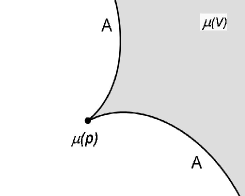
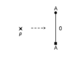
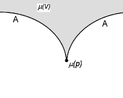
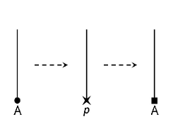
Figure 10. The center-center fixed point. The two possible bifurcation sets and Fomenko graphs near a fixed point of the center-center type.

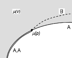
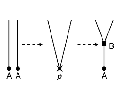
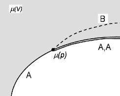
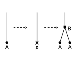
Figure 11. The saddle-center fixed point. The two possible bifurcation sets and Fomenko graphs near fixed point of the saddle-center type.

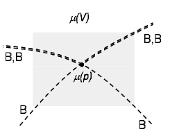
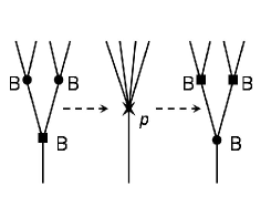
Figure 12. The orientable saddle-saddle fixed point. The two possible bifurcation sets and Fomenko graphs near a fixed point of the saddle-saddle type, when all one-dimensional orbits in its leaf are orientable.

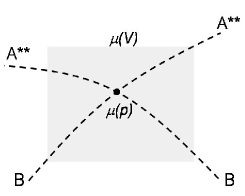
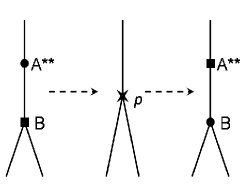
Figure 13. The 4-non-orientable saddle-saddle fixed point. The two possible bifurcation sets and Fomenko graphs near a fixed point of the saddle-saddle type, when all four one-dimensional orbits in its leaf are non-orientable.

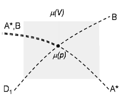
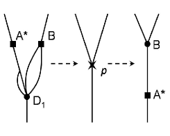
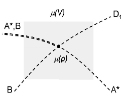
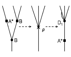
Figure 14. The 3-non-orientable saddle-saddle fixed point. The two possible bifurcation sets and Fomenko graphs near a fixed point of the saddle-saddle type, when three one-dimensional orbits in its leaf are orientable and one is non-orientable.

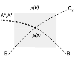
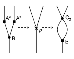
Figure 15. The 2-non-orientable saddle-saddle fixed point. The two possible bifurcation sets and Fomenko graphs near a fixed point of the saddle-saddle type, when two one-dimensional orbits in its leaf are orientable and two are non-orientable.

Figure 16. The focus-focus fixed point. The bifurcation set and the Fomenko graph near a fixed point of the focus-focus type. Notice that this simple diagram corresponds to a countable infinity number of possible r-marked Fomenko graphs, see Remark 7.

Remark 6.

Let us emphasize that, despite the different structures of the isoenergy surfaces foliations, the extended neighborhoods $V$ corresponding to the pairs of subcases shown on Figures 10–15 are isomorphic to each other. In other words, if we consider the Poisson action $\Phi$ without distinguishing $H$ as the Hamiltonian function, these cases do not split into subcases. Therefore, in [10] these cases are identified.

Remark 7.

Fixed points of focus-focus type have interesting monodromy properties, see [20, 22, 63]. In particular, it can be shown that the twisting associated with a focus-focus point can change the $r$-marks of the edge of the graph across this point in a countable infinity number of ways, depending on the way the extended neighborhood of the focus point is glued in the phase space. These infinite number of possible changes in the foliation across the focus point are considered as one type of change in The Singularities and Foliations Theorem.

Next, we describe the changes in the Liouville foliations of the isoenergy surfaces near parabolic circles. Thus we formulate the following consequence of the work [16].

Corollary 8.

Consider a system $(\mathcal{M},\omega,H)$ satisfying Assumptions 1–5 and let $\gamma$ be its parabolic circle. Then, for a sufficiently small extended neighborhood $V$ of $\gamma$, the bifurcation set $\Sigma(V)$ and the corresponding Fomenko graphs are listed by Figures 17, 18, and 19.

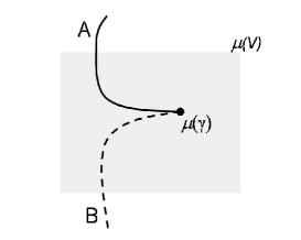
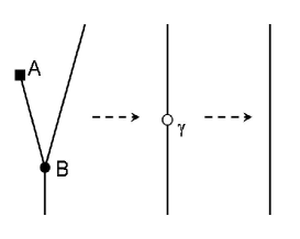
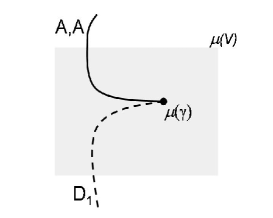
Figure 17. Parabolic circles: the normal form of the family $K_{h}$ is $hx+x^{3}+y^{2}$. Upper line: the bifurcation set and the Fomenko graphs near the saddle-center bifurcation. Lower line: the bifurcation set and the Fomenko graph when two parabolic circles appear simultaneously on the same leaf. Notice the appearance of a curve corresponding to leaves of complexity $2$.

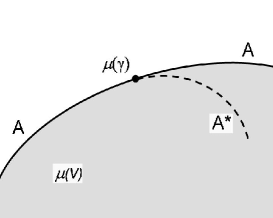
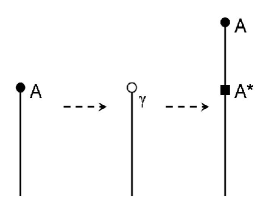
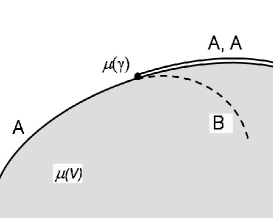
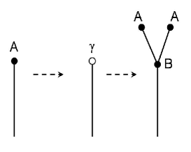
Figure 18. Parabolic circles: the normal form of the family $K_{h}$ is $hx^{2}+x^{4}+y^{2}$. Upper line: the bifurcation set and the Fomenko graphs near elliptic period doubling bifurcation. Lower line: the bifurcation set and the Fomenko graphs near elliptic pitchfork bifurcation.

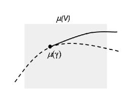
Figure 19. Parabolic circles: the normal form of the family $K_{h}$ is $hx^{2}+x^{4}-y^{2}$. Upper line: the bifurcation set and Fomenko graphs near hyperbolic period doubling bifurcation. Lower line: Fomenko graphs near hyperbolic pitchfork and modified hyperbolic pitchfork bifurcations.

References

- [1] J. M. Arms, J. E. Marsden, V. Moncrief, Symmetry and bifurcations of momentum mappings, Comm. Math. Phys. 78 (1980/81), no. 4, 455–478.
- [2] V. I. Arnol’d, Lectures on bifurcations and versal families, Uspekhi Mat. Nauk 27 (1972), no. 5, 119–184.
- [3] V. I. Arnol’d, Mathematical Methods of Classical Mechanics, Springer-Verlag, New York, 1978.
- [4] T. Bau, N. T. Zung, Singularities of integrable and near-integrable Hamiltonian systems, J. Nonlinear Sci. 7 (1997), 1–7.
- [5] A.R. Bishop, K. Fesser, P. S. Lomdahl, W. C. Kerr, M. B. Williams, and S. E. Trullinger, Coherent spatial structure versus time chaos in a perturbed sine-Gordon system, Phys. Rev. Lett. 50 (1983), 1095–1098.
- [6] A.R. Bishop, M.G. Forest, D.W. McLaughlin, E.A. Overman II, A quasi-periodic route to chaos in a near-integrable pde, Physica D 23 (1986), 293–328.
- [7] A.R. Bishop, P.S. Lomdahl, Nonlinear dynamics in driven, damped sine-Gordon systems, Physica D 18 (1986), 54–66.
- [8] A. Bishop, D.W. McLaughlin, M.G. Forest, E. Overman II, Quasi-periodic route to chaos in a near-integrable PDE: Homoclinic Crossings, Phys. Lett. A 127 (1988), 335–340.
- [9] S. V. Bolotin, D. V. Treschev, Remarks on the definition of hyperbolic tori of Hamiltonian systems, Regul. Chaotic Dyn. 5 (2000), no. 4, 401–412.
- [10] A. V. Bolsinov, Methods for calculations of the Fomenko-Zieschang invariant, in: Topological Classification of Integrable Hamiltonian Systems, Advances in Soviet Mathematics, vol. 6, AMS, Providence, RI, 1991.
- [11] A. Bolsinov, H. R. Dullin, A. Wittek, Topology of energy surfaces and existence of transversal Poincaré sections, J. Phys. A 29 (1996), no. 16, 4977–4985.
- [12] A. V. Bolsinov, A. T. Fomenko, Exact topological classification of Hamiltonian flows on two-dimensional surfaces, Journal of Mathematical Sciences 94 (1999), no. 4, 1457–1476.
- [13] A. V. Bolsinov, A. T. Fomenko, Integrable Hamiltonian Systems: Geometry, Topology, Classification, Chapman and Hall/CRC, Boca Roton, Florida, 2004.
- [14] A. V. Bolsinov, S. V. Matveev, A. T. Fomenko, Topological classification of integrable Hamiltonian systems with two degrees of freedom. List of systems with small complexity, Russian Math. Surveys 45 (1990), no. 2, 59–94.
- [15] A. V. Bolsinov, A. A. Oshemkov, Singularities of integrable Hamiltonian systems, In: Topological Methods in the Theory of Integrable Systems, Cambridge Scientific Publ., 2006, pp. 1–67.
- [16] A. V. Bolsinov, P. H. Richter, A. T. Fomenko, Loop molecule method and the topology of the Kovalevskaya top, Sbornik: Mathematics 191 (2000), no. 2, 151–188.
- [17] H. W. Broer, H. Hanßmann, J. You, Bifurcations of normally parabolic tori in Hamiltonian systems, Nonlinearity 16 (2005), no. 4, 1735-1770.
- [18] H. W. Broer, G. B. Huitema, and M. B. Sevryuk, Quasi-periodic tori in families of dynamical systems: order amidst chaos, vol. 1645 of LNM, Springer Verlag, 1996.
- [19] D. Cai, D.W. McLaughlin, and K.T.R. McLaughlin, The nonlinear Schrödinger equation as both a PDE and a dynamical system, in: Handbook of dynamical systems, Vol. 2, pp. 599–675, North-Holland, Amsterdam.
- [20] R. H. Cushman, L. M. Bates, Global Aspects of Classical Integrable Systems, Birkhauser Verlag AG, 1997.
- [21] N. Desolneux-Moulis, Singular Lagrangian foliation associated to an integrable Hamiltonian vector field, MSRI Publ. 20 (1990), 129–136.
- [22] H. R. Dullin, V. N. San, Vanishing twist near focus-focus points, Nonlinearity 17 (2004), 1777–1785.
- [23] H. R. Dullin, A. Wittek, Efficient calculation of actions, J. Phys. A 27 (1994), no. 22, 7461–7474.
- [24] L. H. Eliasson, Perturbations of stable invariant tori for Hamiltonian systems, Ann. Scuola Norm. Sup. Pisa Cl. Sci. IV 15 (1988), no. 1, 115–147.
- [25] A. T. Fomenko, Topological invariants of Liouville integrable Hamiltonian systems, Functional Anal. Appl. 22 (1988), 286–296.
- [26] A. T. Fomenko, Symplectic topology of integrable dynamical systems. Rough topological classification of classical cases of integrability in the dynamics of a heavy rigid body, Journal of Mathematical Sciences 94 (1999), no. 4, 1512–1557.
- [27] A. T. Fomenko, K. Zieschang, A topological invariant and a criterion for the equivalence of integrable Hamiltonian systems with two degrees of freedom, Izv. Akad. Nauk SSSR Ser. Mat. 54 (1990), no. 3, 546–575.
- [28] V. Gelfreich, Near strongly resonant periodic orbits in a Hamiltonian system, PNAS 99: 13975-13979.
- [29] M. Golubitsky, I. Stewart, Generic bifurcation of Hamiltonian systems with symmetry, Physica D 24 (1987), 391–405.
- [30] S. M. Graff, On the conservation of hyperbolic invariant tori for Hamiltonian systems, J. Diff. Eq. 15 (1974), 1–69.
- [31] J. Guckenheimer, P. Holmes, Nonlinear Oscillations, Dynamical Systems, and Bifurcations of Vector Fields, New York: Springer, 1983.
- [32] G. Haller, Chaos near Resonance, Springer-Verlag, NY, 1999.
- [33] H. Hanßmann, Local and Semi-Local Bifurcations in Hamiltonian Dynamical Systems, Springer, 2007.
- [34] G. Haller, S. Wiggins. Orbits homoclinic to resonances: The Hamiltonian case, Physica D 66 (1993), 298–346.
- [35] V. V. Kalashnikov, Typical integrable Hamiltonian systems on a four-dimensional symplectic manifold, Izvestiya: Mathematics 62 (1998), no. 2, 261–285.
- [36] G. Kovačič, Singular perturbation theory for homoclinic orbits in a class of near-integrable dissipative systems, J. Dynamics Diff. Eqns. 5 (1993), 559–597.
- [37] L. M. Lerman, Isoenergetical structure of integrable Hamiltonian systems in an extended neighborhood of a simple singular point: three degrees of freedom, Methods of qualitative theory of differential equations and related topics, Supplement, 219–242, Amer. Math. Soc. Transl. Ser. 2, 200, Amer. Math. Soc., Providence, RI, 2000.
- [38] L. M. Lerman, Ya. L. Umanskiy, Four-Dimensional Integrable Hamiltonian Systems with Simple Singular Points (Topological Aspects), Translations of mathematical monographs, volume 176, AMS, 1998.
- [39] A. Lichtenberg, M. Lieberman. Regular and Stochastic Motion. Springer, New York, NY, 1983.
- [40] A. Litvak-Hinenzon, V. Rom-Kedar, Parabolic resonances in degree of freedom near-integrable Hamiltonian systems, Phys. D 164 (2002), no. 3-4, 213–250.
- [41] A. Litvak-Hinenzon, V. Rom-Kedar, Resonant tori and instabilities in Hamiltonian systems, Nonlinearity 15 (2002), no. 4, 1149–1177.
- [42] A. Litvak-Hinenzon, V. Rom-Kedar, On energy surfaces and the resonance web, SIAM J. Appl. Dyn. Syst. 3 (2004), no. 4, 525–573.
- [43] R. de la Llave, C. E. Wayne, Whiskered and low dimensional tori in nearly integrable Hamiltonian systems, Math. Phys. Electron. J. 10 (2004), Paper 5, 45 pp.
- [44] L. Markus, K. R. Meyer, Generic Hamiltonian dynamical systems are neither integrable nor ergodic, Memoirs of the American Mathematical Society, no. 144, AMS, Providence, R.I., 1974.
- [45] J. R. Marsden, A. Weinstein, Reduction of symplectic manifolds with symmetry, Reports Math. Phys. 5 (1974), no. 1, 121–130.
- [46] S. V. Matveev, Integrable Hamiltonian systems with two degrees of freedom. The topological structure of saturated neighbourhoods of points of focus-focus and saddle-saddle type, Sbornik: Mathematics 184 (1996), no. 4, 495–524.
- [47] S. V. Matveev, A. T. Fomenko, Algorithmic and Computer Methods in Three-Dimensional Topology, Moskov. Gos. Univ., Moscow, 1991.
- [48] K. R. Meyer, R. G. Hall, Introduction to Hamiltonian Dynamical Systems and the N-Body Problem, volume 90 of Applied Mathematical Sciences. Springer-Verlag, NY, 1991.
- [49] J. Moser, Dynamical Systems - Past and Present, Documenta Mathematica - Extra Vol ICM 1998, I pp 381–402, 1998.
- [50] N. N. Nekhoroshev, The action-angle variables and their generalizations, Trudy Moskov. Mat. Obshch. 26 (1972), 181–198.
- [51] O. E. Orel, P. E. Ryabov, Topology, bifurcations and Liouville classification of Kirchhoff equations with an additional integral of fourth degree, J. Phys. A 34 (2001), no. 11, 2149–2163. Kowalevski Workshop on Mathematical Methods of Regular Dynamics (Leeds, 2000).
- [52] A. A. Oshemkov, Fomenko invariants for the main integrable cases of the rigid body motion equations, in: Topological Classification of Integrable Hamiltonian Systems, Advances in Soviet Mathematics, vol. 6, AMS, Providence, RI, 1991.
- [53] J. Pöschel, On elliptic lower dimensional tori in Hamiltonian systems, Math. Z. 202 (1989), 559–608.
- [54] J. Sanders, F. Verhulst, Averaging methods in nonlinear dynamical systems, In Applied Mathematical Sciences, volume 59, Springer-Verlag, New York, NY, 1985.
- [55] E. Shlizerman, V. Rom-Kedar, Hierarchy of bifurcations in the truncated and forced nonlinear Schrödinger model, Chaos 15 (2005), no. 1.
- [56] E. Shlizerman, V. Rom-Kedar, Three types of chaos in the forced nonlinear Schrödinger equation, PRL 96, 024104, 2006.
- [57] S. Smale, Topology and mechanics. I, Inventiones math. 10 (1970), 305–331.
- [58] S. Smale, Topology and mechanics. II, the planar -body problem, Inventiones math. 11 (1970), 45–64.
- [59] F. Verhulst, Symmetry and integrability in Hamiltonian normal forms, In Symmetry and Perturbation Theory (Editors: D. Bambusi, G. Gaeta), Quaderni GNFM, Firenze, 1998, pages 245–284.
- [60] J. Williamson, On the algebraic problem concerning the normal forms of linear dynamical systems, Amer. J. Math. 58 (1936), no. 1, 141–163.
- [61] G. Zaslavsky, R. Sagdeev, D. Usikov, and A. Chernikov. Weak Chaos ans Quasiregular Patterns, Cambridge University Press, Cambridge, 1991.
- [62] N. T. Zung, Symplectic topology of integrable Hamiltonian systems, I: Arnold-Liouville with singularities, Comp. Mathematica 101 (1996), 179–215.
- [63] N. T. Zung, A note on focus-focus singularities, Differential Geom. Appl. 7 (1997), 123–130.
- [64] N. T. Zung, A note on degenerate corank-one singularities of integrable Hamiltonian systems, Comment. Math. Helv. 75 (2000), 271–283.
- [65] N. T. Zung, Symplectic topology of integrable Hamiltonian systems, II: Topological Classification, Comp. Mathematica 138 (2003), 125–156.