Nodal Domain Distribution for a Nonintegrable Two-Dimensional Anharmonic Oscillator

Abstract

We investigate the transition from integrable to chaotic dynamics in the quantum mechanical wave functions from the point of view of the nodal structure by employing a two dimensional quartic oscillator. We find that the number of nodal domains is drastically reduced as the dynamics of the system changes from integrable to nonintegrable, and then gradually increases as the system becomes chaotic. The number of nodal intersections with the classical boundary as a function of the level number shows a characteristic dependence on the dynamics of the system, too. We also calculate the area distribution of nodal domains and study the emergence of the power law behavior with the Fisher exponent in the chaotic limit.

PACS number: 05.45.Mt, 64.60.Ak

I Introduction

Quantum signatures of classically chaotic systems have been intensively studied and are now known to have some universal features in the energy level statistics. Similar investigations on the signatures in the wave functions which may distinguish chaotic systems from integrable ones have also been performed[1, 2]. A related signature of chaotic systems is given by the amplitude distribution of wave functions which empirically reproduces the results of random matrix theory [3].

Recently, it was suggested in Ref. [4] that there is in fact such a universal character in the statistics of nodal domains of wave functions. The authors of Ref. [4] calculated the number of nodal domains $N_{i}$ of the $i$th wave function, i.e., the regions where the wave function has a definite sign without crossing zeros, for two-dimensional billiards. They showed that the distribution of normalized number $N_{i}/i$ of nodal domains for separable systems has a universal feature characterized by a square root singularity, while that for chaotic billiards shows a completely different behavior, suggesting a scaling law $N_{i}\approx i$ for large $i$. The latter scaling law has been derived in Ref. [5], where the authors adopted a percolation-like model to count the number of nodal domains. The authors of Ref.[5] analytically derived the scaling law for the average number of nodal domains and showed that it agrees well with the numerical results for the superposition of random waves, i.e., a model which is supposed to simulate the wave functions for chaotic billiards[1]. The percolation-like model allowed them to predict a power law behavior for the distribution of nodal domain areas, and also the fractal dimension of nodal domains. These predictions were shown to agree well with the numerical results for the superposition of random waves, although one may not conclude from these results alone that the area distribution provides a clear signature of quantum chaoticity. The number of nodal domains was studied also experimentally for the chaotic microwave billiard [6].

In the above studies of nodal domains, the two extremes of dynamical systems, completely integrable (separable) and chaotic (or its alternative), have been considered. It is the purpose of the present paper to extend these studies to a more general nonintegrable system, where, by controlling a parameter in the Hamiltonian, one can interpolate the two extremes. We expect this would show the transition from integrable to chaotic systems for the nodal domain distribution and thus may provide a clue to the role of nonintegrable perturbation which was implicit in the percolation-like model. We expect that a study of the power law behavior of nodal domain areas would also give a suggestion on the validity of the assumption adopted in the model.

Below we first describe the model and the numerical procedure. We present numerical results for the distribution of nodal domain numbers in Sec. III together with some analytical considerations. The distribution of the nodal intersections with the boundary of the classically allowed region is presented in Sec. IV. Results for the distribution of nodal domain areas are given in Sec. V. Proofs of formulas and some details of the calculations in the text are given in the Appendices.

II Model and Numerical Procedure

As a model which incorporates integrable as well as almost chaotic systems, we adopt a two-dimensional quartic oscillator

$$H=\frac{1}{2}(p_{x}^{2}+\alpha p_{y}^{2})+V(x,y),$$ (1)

$$V(x,y)=\frac{1}{2}(x^{4}+y^{4})-kx^{2}y^{2},$$ (2)

where the parameter $k$ controls the dynamics of the system. Detailed studies performed at $\alpha=1$ shows that the classical dynamics of the system at $k=0.0$ is integrable, becomes irregular as the value of $k$ increases, and reaches an almost chaotic system at $k=0.6$[7]. The energy level statistics of the quantum mechanical system show a similar transition, e.g., from Poisson to Wigner level spacing distribution as $k$ increases[8]. The parameter $\alpha$ is introduced to break the symmetry with respect to the exchange of the $x$ and $y$ coordinates, which otherwise leads to an ambiguity in the definition of the eigenfunction at $k=0.0$. The value of $\alpha$ is set to the value 1.01 throughout. We plot in Fig. 1 the Poincarè surface of section for the system with $\alpha=1.01$ at several values of $k$. Qualitative behavior is almost the same as that with $\alpha=1$.

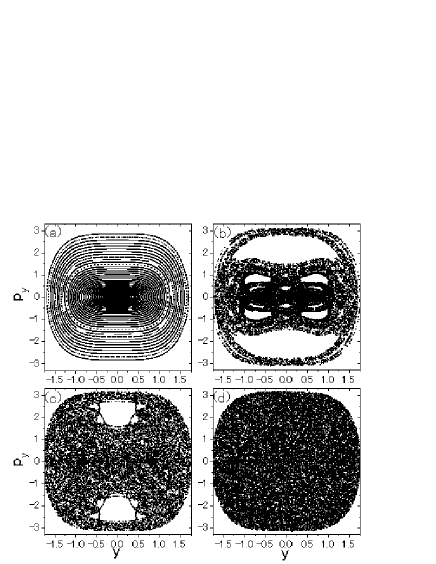
FIG. 1.: Poincarè surface of section for the system of the Hamiltonian Eq. (2) with $\alpha=1.01$ at $E=5.0$, $x=0.0$, and (a) $k=0.0$, (b) 0.2, (c) 0.4, (d) 0.6. The abscissa axis represents $y$ coordinate and the ordinate $p_{y}$.

In the numerical calculation, we first diagonalize the Hamiltonian in a large harmonic oscillator (h.o.) basis and obtain wave functions for eigenstates. To determine nodal domains we cut the two-dimensional sheet into small squares (meshes) so that they cover the allowed region of classical motion for each eigenvalue. We then study the sign of the wave function at each center of a mesh, and calculate the number of nodal domains by means of the Hoshen-Kopelman algorithm [9]. Here, two nearest neighbor meshes with the same sign are considered to belong to the same nodal domain. The size of the mesh is then changed to a smaller value until the convergence of the number of nodal domains is obtained. Adopted value of the mesh size is $x_{\rm cl}(E_{i})/\max(1.4i,200)$ for the $i$th eigenstate with energy $E_{i}$, where $x_{\rm cl}(E)$ represents the largest value of the $x$ coordinate for a classical motion with energy $E$. One should note that the method becomes inaccurate for very small values of $k$, where the nodal crossing changes to a small avoided crossing due to the nonseparable perturbation. The smallest positive value of $k$ in the present paper is 0.06 which was used in Sec. III C to study the qualitative behavior of the number of nodal domains by comparing with a perturbative argument.

Contrary to the case of the billiards, the size of the meshed sheet in the present case is not a priori determined. In fact, since there is no hard wall, wave functions extend to infinity. They are, however, rapidly attenuated beyond classically allowed region for given energy. Moreover, as shown in Appendix A, there appears no new nodal domain in the classically forbidden region. Therefore, we adopted the meshed sheet whose boundary coincides with that of the classically allowed region. All nodal domains, then, have an overlap with the meshed sheet. In case that the boundary of the meshed sheet cuts a nodal domain into several pieces the number of nodal domains may be overestimated due to the choice of the meshed sheet. To estimate the error caused by this boundary effect, we evaluated the difference between the number of nodal domains in the adopted meshed sheet and that in the square sheet that circumscribes the classically allowed region. The estimated difference was 3.1% for $k=$0.1 and 2.2% for $k=$0.6.

The Hamiltonian is still symmetric with respect to the $x$-axis and the $y$-axis[7]. We calculated only those wave functions which are symmetric with respect to these two axes. The diagonalization space was truncated at $n_{x}+n_{y}\leq 200$, where $n_{x}$ and $n_{y}$ denote the numbers of oscillator quanta in the $x$- and $y$-directions. The adopted oscillator frequency in the diagonalization was optimized so as to minimize the value of ${\rm Tr}H$ in this space for each $k$ value[10].

When $k=0.0$, we can obtain more accurate numerical results by adopting product of the wave functions for one-dimensional quartic oscillator calculated in a similar diagonalization procedure. Comparison of the number of nodal domains obtained in the two methods may provide a rough estimate for the accuracy of the adopted diagonalization procedure, which in the present case is less than 2.4%. For the $k=0.0$ results presented below we adopt those obtained by the product wave functions.

III Distribution of the Number of Nodal Domains

A General consideration on the number of nodal domains

Before discussing the nodal structure for the present model, it is useful to study general properties of the number of nodal domains which provide a useful classification scheme to be used in later sections.

The number of nodal domains $N$ for a given nodal line structure of a wave function in a two-dimensional area with a boundary $B$ is given by the formula

$$N(n_{b},n_{c},m)=\frac{1}{2}n_{b}+n_{c}+m+1,$$ (3)

under the assumption that more than two nodal lines never cross at the same crossing point. In Eq. (3), $n_{b}$ represents the number of intersections of nodal lines with the boundary $B$, $n_{c}$ the number of crossing points of nodal lines, and $m$ the number of islands. Here, the term ‘island’ means a cluster of mutually connected nodal lines which is linked neither to $B$ nor to other clusters. A similar formula to (3) has been used and proved in Ref. [11] in a slightly different setting of the problem to study the multiplicity of eigenvalues for a membrane. In Appendix B we give a proof of the relation (3) for completeness.

We discuss two cases in which this formula is especially useful. The first is the $m=0$ case, i.e., the case where all nodal lines are linked to the boundary, which is typical for separable (and therefore integrable) system. In this case

$$N=\frac{1}{2}n_{b}+n_{c}+1.\quad\mbox{(separable, generic)}$$ (4)

This allows us to discuss the dependence of $N$ on the level number in relation to the structure of the wave function for $k=0.0$ as shown below.

The second case is $n_{c}=0$ which corresponds to the generic wave function of nonintegrable systems, where almost all crossings of nodal lines change to avoided crossings except for an accidental case. We may first rewrite the number of nodal domains in Eq. (3) as the sum of two terms:

$$N=N^{\rm in}+N^{b},$$ (5)

where $N^{\rm in}$ denotes the number of ‘inner nodal domains’, i.e., those which do not touch the boundary $B$, while $N^{b}$ denotes the remaining part, i.e., the number of ‘ boundary nodal domains’ which touch the boundary $B$. If there is no crossing, $n_{c}=0$, it is easy to see that $N^{\rm in}$ is equal to the number $m$ of islands. From Eq. (3), then, we find for $n_{c}=0$

$$N^{\rm in}=m,\quad N^{b}=\frac{1}{2}n_{b}+1.\qquad\mbox{(nonintegrable, generic)}$$ (6)

The generic relation Eq. (6) for the number of boundary nodal domains may provide an estimate on the number of false crossing of nodal lines due to the finite mesh size in the numerical calculation. Comparison of the value of $N^{b}$ with the one obtained from the value of $n_{b}$ gives a difference of 5.2% for $k=$0.1  and 2.5% for $k=$0.6.

FIG. 2.: Number of nodal domains $N_{i}$ vs. the level number $i$ for (a) $k=0.0$, (b) 0.1, (c) 0.2, (d) 0.3, (e) 0.4, (f) 0.5, and (g) 0.6. Solid lines show the function $f(i)$, while the dashed lines the function $\tilde{f}(i)$. See text for details.

B Numerical results for the distribution of the number of nodal domains

Figure 2 shows the distribution of the number of nodal domains, $N_{i}$, where the subscript $i$ stands for the level number ordered according to the eigenvalue. Note that the quoted level number $i$ is not the one of the total system, since we consider only levels which are symmetric with respect to the $x$ axis and the $y$ axis. In the present model, there are four symmetry classes, and the eigenvalues in the four classes are almost equally distributed. In the space $n_{x}+n_{y}\leq 200$ the total number of levels is 20301 and that in the adopted symmetry class is 5151. Thus, we may assign for each $i$ the corrected level number $i^{\prime}$ approximately given by $i^{\prime}=ci$ with $c=20301/5151$. The solid lines in Fig. 2 represent the prediction according to the percolation-like model which is given by the following function:

$$f(i)={3\sqrt{3}-5\over 2}\beta i^{\prime},$$ (7)

where the value of the coefficient $\beta$ is taken as $2/\pi$ as calculated for the billiard model [5]. In the percolation-like model, one first considers a nodal structure of the rectangular lattice pattern, and then assumes that an avoided crossing of nodal lines occur at every lattice point randomly, i.e., either of the positive or negative domains is connected at the point with probability 1/2 independent of the other lattice points. Figure 3 shows a nodal domain distribution represented as a histogram vs. $N_{i}/i^{\prime}$. We give in Table I the average and the standard deviation of $N_{i}/i^{\prime}$.

FIG. 3.: Histogram of $N_{i}/i^{\prime}$ for (a) $k=0.0$, (b) 0.1, (c) 0.2, (d) 0.3, (e) 0.4, (f) 0.5, and (g) 0.6, where $i^{\prime}$ stands for the corrected level number.

We first discuss the $k=0.0$ case where the system is separable. In this case the eigenfunction is given by $\psi_{mn}(x,y)=\phi_{m}(x)\phi_{n}(y)$, where $\phi_{m}(x)$ represents the $m$th wave function of a one-dimensional quartic oscillator in the $x$-direction. The behavior of the histogram in Fig. 3 (a) is similar to the one for the integrable system given in Ref. [4], showing an increase and a sharp cut-off at some value of $N_{i}/i^{\prime}$. By inspecting Fig. 2 (a) we find that this behavior comes from a number of regular sequences of eigenstates. The sequence with the largest $N_{i}$ values is proportional to $i$, and the corresponding wave functions have the form $\psi_{nn}(x,y)$. This may be contrasted to the sequence with the smallest $N_{i}$ values which is proportional to $\sqrt{i}$ as shown by the dashed line in Fig. 2 (a). The wave functions in this sequence are of the form $\psi_{n1}(x,y)$ or $\psi_{1n}(x,y)$. The slopes of other sequences are intermediate between them. Typical nodal structures corresponding to $\psi_{nn}(x,y)$ and $\psi_{n1}(x,y)$ are shown in Fig. 4.

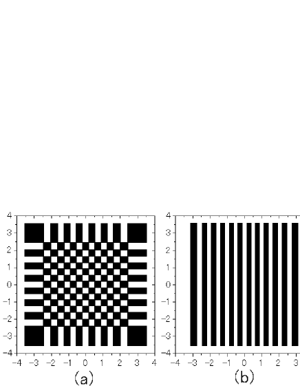
FIG. 4.: Nodal structures of wave functions at $k=0.0$: (a) An example of $\psi_{nn}(x,y)$ ($i=98$, $N^{\rm in}_{i}=169$, $N^{b}_{i}=56$) and (b) an example of $\psi_{n1}(x,y)$ ($i=103$, $N^{\rm in}_{i}=0$, $N^{b}_{i}=25$).

TABLE I.: Average and standard deviation of $N_{i}/i^{\prime}$ distribution (total) and those of $N^{\rm in}_{i}/i^{\prime}$ distribution (inner, see the text) for each $k$. Levels $1\leq i\leq 1000$ are considered.

	total		inner
$k$	Ave.	S.D.	Ave.	S.D.
0.0	0.37	0.17	0.29	0.17
0.1	0.049	0.035	0.014	0.013
0.2	0.051	0.035	0.022	0.016
0.3	0.055	0.034	0.031	0.018
0.4	0.063	0.032	0.042	0.019
0.5	0.071	0.030	0.052	0.018
0.6	0.079	0.029	0.060	0.017

FIG. 5.: Number of inner nodal domains $N^{\rm in}_{i}$ vs. the level number $i$ for (a) $k=0.0$, (b) 0.1, (c) 0.2, (d) 0.3, (e) 0.4, (f) 0.5, and (g) 0.6. Solid lines show the function $f(i)$.

These behaviors may be understood from Eq. (4). For eigenfunctions of the form $\psi_{n1}(x,y)$ there is no crossing, $n_{c}^{(i)}=0$, thus $N_{i}\simeq n_{b}^{(i)}/2$. (Below we explicitly write the $i$ dependence of $n_{b}$.) Since $n_{b}^{(i)}$ is proportional to $\sqrt{i}$ [4], the number of nodal domains $N_{i}$ in the lowest sequence is also proportional to $\sqrt{i}$. The dashed line in Fig. 2 shows the function

$${\tilde{f}}(i)=d\sqrt{i^{\prime}},~{}~{}d=\frac{2\pi^{1/4}}{\sqrt{3}\Gamma({3\over 4})}\simeq 1.25,$$ (8)

which represents the number of nodal domains for wave functions $\psi_{n1}(x,y)$ evaluated in a semiclassical way as given in Appendix C 1. On the other hand, for eigenfunctions of the type $\psi_{nn}(x,y)$, the number of crossing is given by $n_{c}^{(i)}=(n_{b}^{(i)})^{2}/4$, and $N_{i}$ is dominated by $n_{c}^{(i)}$ if $n_{b}^{(i)}$ is large enough. Accordingly, $N_{i}$ in the highest sequence is proportional to $i$. Note that when the level number $i$ becomes larger, in almost all levels the contribution of $n_{c}$ becomes dominant, and the number of nodal domains $N_{i}$ becomes proportional to $i$ on average.

When the value of $k$ becomes nonzero, e.g., $k=0.1$ in Fig. 2 (b), the number of nodal domains is drastically reduced. This is due to the transition from the crossing to the avoided crossing of nodal lines. The shape of the histogram in Fig. 3 (b) changes, too: The peak at the highest value of $N_{i}/i^{\prime}$ at $k=0.0$ disappears and the histogram is now largely shifted towards low values of $N_{i}/i^{\prime}$.

FIG. 6.: Number of boundary nodal domains $N^{b}_{i}$ vs. the level number $i$ for (a) $k=0.0$, (b) 0.1, (c) 0.2, (d) 0.3, (e) 0.4, (f) 0.5, and (g) 0.6. Dashed lines show the function $\tilde{f}(i)$.

To see more details, we plot $N^{\rm in}_{i}$ and $N^{b}_{i}$ in Figs. 5 and 6, respectively. From these figures, we see that at $k=0.1$ the number of inner nodal domains drastically decreases below the $f(i)$ line, while the distribution of the number $N^{b}$ of boundary nodal domains tends to accumulate around the ${\tilde{f}}(i)$ line. These together lead to the reduction of the total number of nodal domains compared with the separable case at $k=0.0$. The $k$-dependence of $N^{\rm in}_{i}$ and that of $N^{b}_{i}$ are, however, quite different. As $k$ becomes larger, the number of boundary nodal domains decreases further and eventually becomes rather a small fraction of the total number of domains except at low energy (small $i$) region. In contrast, the number of inner nodal domains increases again, and in the chaotic limit around $k=0.6$ almost aligns to the $f(i)$ line as in the case of the billiard system. Typical nodal structure for a wave function at $k=0.6$ is shown in Fig. 7.

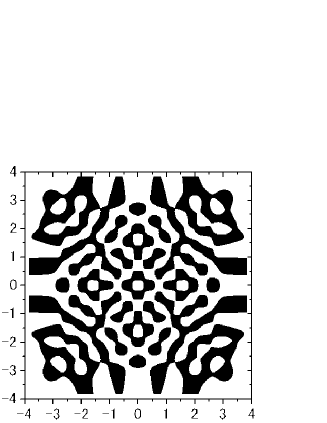
FIG. 7.: Nodal structure of the 102nd wave function at $k=0.6$, where $N^{\rm in}_{i}=30$ and $N^{b}_{i}=17$.

Let us further study the behavior of the number of inner nodal domains $N^{\rm in}_{i}$. We show the histogram of $N^{\rm in}_{i}/i^{\prime}$ in Fig. 8, and the average and the standard deviation of $N^{\rm in}_{i}/i^{\prime}$ in Table I. The peak position of the histogram suddenly drops almost to zero as $k$ becomes nonzero, which suggests that the nonintegrability first acts in such a way to eliminate inner nodal domains. This behavior is studied in the next subsection using perturbative argument. The peak of $N^{\rm in}_{i}/i^{\prime}$ then gradually increases with $k$, and finally the shape becomes approximate Gaussian at $k=0.6$ centered at finite value of $N^{\rm in}_{i}/i^{\prime}$, but still is much smaller than the case of $k=0.0$. Accordingly, the average of $N^{\rm in}_{i}/i^{\prime}$ increases. The behavior of the histogram of total nodal domains at finite $k$ in Fig. 3 follows that of the inner nodal domains.

The number of boundary nodal domains $N^{b}_{i}$ in Fig. 6 also shows interesting features. At $k=0.0$ there are two regular sequences. The sequence with larger values corresponds to the wave functions $\psi_{mn}=\phi_{m}(x)\phi_{n}(y)$ $(m\neq 1,n\neq 1)$, while the sequence with smaller values to the wave functions $\psi_{n1}$ or $\psi_{1n}$. In the latter wave functions nodal domains have a one-dimensional structure, while in the former the boundary nodal domains are systematically aligned along the boundary. Both sequences are proportional to the square root of the level number $\sqrt{i}$. In Fig. 6, we show the function ${\tilde{f}}(i)$ in Eq. (8) by the dashed line. For small $k$ values, say $k=0.1$, the number of boundary nodal domains is distributed around the ${\tilde{f}}(i)$ line.

FIG. 8.: Histogram of $N^{\rm in}_{i}/i^{\prime}$for (a) $k=0.0$, (b) 0.1, (c) 0.2, (d) 0.3, (e) 0.4, (f) 0.5, and (g) 0.6, where $i^{\prime}$ stands for the corrected level number.

C Reduction of the number of nodal domains in the perturbative regime

When the dynamics changes from integrable to nonintegrable, crossing of nodal lines changes to avoided crossing, which leads to the reduction of the number of nodal domains. However, this alone is not sufficient to explain the difference in the reduction at small $k$ value and that at large $k$ value as seen in Figs. 5 and 6.

Figure 9 shows distributions of $N_{i}$, $N^{\rm in}_{i}$, $N^{b}_{i}$, and the histogram of $N^{\rm in}_{i}/i^{\prime}$ at $k=0.06$. We see that the number of inner nodal domains is smaller than the case of $k=0.1$, while the number of boundary nodal domains remains approximately the same. This further confirms that the number of inner nodal domains becomes smaller as the value of $k$ decreases as long as the value is nonzero. As noted above the avoided crossing becomes weaker as the value of $k$ decreases. Accordingly, the smaller mesh-size is required to avoid the fictitious crossing. Indeed, we used the mesh size $x_{\rm cl}(E_{i})/\max(3.0i,200)$ for the calculation at $k=0.06$. Properties of the avoided crossing (avoidance range) have been studied in Ref. [12].

FIG. 9.: Number of different kinds of nodal domains at $k=0.06$ is shown against the level number $i$ : (a) Number of total nodal domains $N_{i}$, (b) number of inner nodal domains $N^{\rm in}_{i}$, and (c) number of boundary nodal domains $N^{b}_{i}$. Histogram of $N^{\rm in}_{i}/i^{\prime}$ is shown in (d). Solid lines in (a) and (b) show the function $f(i)$, while dashed line in (a) and (c) the function $\tilde{f}(i)$.

When the value of $k$ is small, wave functions may well be approximated by the 1st order perturbation theory. The perturbed wave function can be written as,

$$\psi^{\prime}_{mn}(x,y) = \psi_{mn}(x,y)+k\sum_{(m^{\prime},n^{\prime})\neq(m,n)}C_{m^{\prime}n^{\prime}}\psi_{m^{\prime}n^{\prime}}(x,y),$$ (9)

$$C_{m^{\prime}n^{\prime}} = \frac{\langle\psi_{m^{\prime}n^{\prime}}|x^{2}y^{2}|\psi_{mn}\rangle}{E_{m^{\prime}n^{\prime}}-E_{mn}},$$ (10)

where $E_{mn}$ represents an unperturbed energy. Because of the second term, the crossing of nodal lines in the unperturbed wave function $\psi_{mn}$ will in generic case turn to an avoided crossing. Whether the positive domains or the negative ones are connected and merged into one nodal domain at this avoided crossing depends on the sign of the second term of (10) at the nodal crossing point of $\psi_{mn}$. Note that if this merging occurs randomly independent of the crossing points as in the percolation-like model, one would not obtain such a huge reduction of the number of inner nodal domains as seen in Fig. 9. This suggests that there is a correlation in the sign of the second term among different nodal crossing points of $\psi_{mn}$. The sign of the second term is mainly governed by the sign of the sum of a few principal components which have the largest values of $|C_{m^{\prime}n^{\prime}}|$. For instance, we verified that the probability of the sign of the sum of two principal components to be equal to that of the total second term at randomly chosen points $(x,y)$ is 0.86 for the present model. Moreover, the difference between the $x$ quantum number of a principal component $m^{\prime}$ and that of the unperturbed wave function $m$, is generally very small compared with $m$: $|\delta m|\equiv|m^{\prime}-m|\ll m$, as long as $m$ is large. The same argument holds for the quantum number $n$ in the $y$ direction.

We now evaluate the correlation between signs of a principal component with the $x$ quantum number $m^{\prime}$ at two neighboring crossing points along the $x$-direction. The distance $d$ between two neighboring crossing points is the typical half wavelength $\frac{1}{2}\lambda_{m}$ for the quartic oscillator wave function $\phi_{m}$. Suppose first that the distance $d$ is shorter than the half wavelength $\frac{1}{2}\lambda_{m^{\prime}}$ of the principal component. Then, two neighboring crossing points must belong to the same half wavelength region in order that signs of the principal component at these two neighboring crossing points are same. Thus, the probability $P_{\rm s}$ that the signs of the principal components at two neighboring crossing points to be same can be estimated as

$$P_{\rm s}=\frac{\lambda_{m^{\prime}}-\lambda_{m}}{\lambda_{m^{\prime}}}=\frac{|\delta m|}{m},$$ (11)

where we used an approximate relation $\lambda_{m}\propto m^{-1}$. When the distance $d$ is larger than the half wavelength $\frac{1}{2}\lambda_{m^{\prime}}$, the probability $P_{\rm s}$ can also approximately be given by Eq. (11). A superposition of a few principal components also has a wavelength close to the unperturbed one $\lambda_{m}$, leading to the same result. Above argument can also be applied to the $y$-direction.

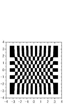
FIG. 10.: Nodal structure of the 92nd wave function at $k=0.06$, where $N^{\rm in}_{i}=0$ and $N^{b}_{i}=27$.

Eq. (11) shows that the probability $P_{\rm s}$ is much less than unity. This means that nodal domains in the unperturbed wave function tend to be connected along the diagonal when a small perturbation is added, which results in the reduction of the number of inner nodal domains. Figure 10 shows a typical nodal pattern at $k=0.06$. We see that unperturbed nodal domains, which are slightly deformed from rectangular, are indeed connected along a diagonal direction. (Compare with Fig. 4 (a), where $N^{\rm in}_{i}$ dominates.) This result supports the above consideration.

For large $k$ values, the perturbation theory becomes no longer a good approximation, and the above discussion cannot be applied.

D Model for the distribution of the number of nodal domains in the chaotic regime

As a reference to the number of nodal domains, we used the function $f(i)$ Eq. (7) derived for the chaotic billiard model [5]. As previously noted, in the percolation-like model, one first considers nodal structure of the rectangular lattice pattern. In order to determine the size of lattice, the relation $k_{x}^{2}=k_{y}^{2}=E$ was used in Ref. [5], where $k_{x}$ denotes the wave number of $x$-axis. This relation is, however, specific to billiard models. Thus, if a system has a potential as in the present case, the distribution of the number of nodal domains may differ from billiard models even in the chaotic regime. Therefore, we would like to present a semiclassical model which provides a more general expression for the nodal domain distribution incorporating some features of a Hamiltonian with a local potential.

Let us first summarize the results obtained in Ref. [4] for separable systems, where the Hamiltonian $H$ is specified by two action variables $I_{1},I_{2}$. According to them, the distribution function of $N_{i}/i$ in a region $E_{1}\leq E_{i}\leq E_{2}$ (which we call $A$) in the $I_{1}-I_{2}$ plane can be written as,

$$P(\xi)=\frac{1}{N_{A}}\int_{I_{1},I_{2}\in A}dI_{1}dI_{2}\delta\left(\xi-\frac{\nu(I_{1},I_{2})}{N(E)}\right),$$ (12)

where $N(E)$ is the semiclassical number of levels

$$N(E)=\int dI_{1}dI_{2}\Theta\left(E-H(I_{1},I_{2})\right),$$ (13)

up to energy $E$, $N_{A}=N(E_{2})-N(E_{1})$ the number of levels in the region $A$, and $\nu(I_{1},I_{2})=I_{1}I_{2}$ is the number of nodal domains of the eigenstate specified by $I_{1},I_{2}$. Assuming that the Hamiltonian is a homogeneous function of $I_{1}$ and $I_{2}$, we transform the variables from $I_{1}$ and $I_{2}$ to the energy $E$ and $r$, where $r$ represents the length of the path along the arc $\Gamma$ with $E=1$ measured from the edge on the $I_{2}$ axis. The action variables are written in terms of the new variables as $(I_{1},I_{2})=(g(E)I^{(0)}_{1}(r),g(E)I^{(0)}_{2}(r))$, where $I^{(0)}_{1}(r)$ and $I^{(0)}_{2}(r)$ represent the action on the arc $\Gamma$. When the Hamiltonian is a function of the $\ell$th order in $I_{1}$ and $I_{2}$, $g(E)=E^{1/\ell}$. The Jacobian of the transformation is given by the product $J(E)L(r)$,

$$J(E) = 2\,g(E){dg(E)\over dE},$$ (14)

$$L(r) = \frac{1}{2}\,\left|\frac{dI^{(0)}_{1}(r)}{dr}I^{(0)}_{2}(r)-\frac{dI^{(0)}_{2}(r)}{dr}I^{(0)}_{1}(r)\right|.$$ (15)

With these variables, the number of levels $N(E)$ is given by

$$N(E)=\left\{g(E)\right\}^{2}N(1),\qquad N(1)=\int L(r)dr.$$ (16)

By performing the $E$-integration, one obtains the result of Ref. [4]:

$$P(\xi)=\frac{1}{N(1)}\int_{\Gamma}dr\,L(r)\delta\left(\xi-\frac{I^{(0)}_{1}(r)I^{(0)}_{2}(r)}{N(1)}\right).$$ (17)

In order to treat the nonintegrable cases, we modify the expression (12) so as to include the following features:

• Hamiltonian is not simply a function of $I_{1},I_{2}$ alone but depends also on the angle variables.

• Number of nodal domains for a given energy is reduced on the average due to nonintegrability.

The first feature implies that each state is not specified by a point $I_{1},I_{2}$ in the phase space, but is distributed over an area with fixed $E$ when projected on the $I_{1}-I_{2}$ plane. We may include this effect by replacing the variable $r$ involved in $\nu$ with the smoothed one $r_{\omega}(r)$;

$$r_{\omega}(r)\equiv\int_{0}^{r_{\rm max}}f_{\omega}(r,r^{\prime})r^{\prime}dr^{\prime},$$ (18)

where, $f_{\omega}(r,r^{\prime})$ represents a smoothing function with the width $\omega$, and $r_{\rm max}$ the total length of the arc $\Gamma$. The width $\omega$ would correspond to the degree of the amplitude mixing of the wave function when expanded in the basis of the integrable system. For the integrable system, $\omega=0$, and when the system is chaotic, the wave function will be distributed over the available phase space, i.e., $\omega\geq r_{\rm max}$. The second feature ii) may be included by an introduction of a reduction factor $G$, i.e.,

$$\nu(I_{1},I_{2})\quad\rightarrow\quad I_{1}I_{2}G(I_{1},I_{2})$$ (19)

with $G=1$ for separable systems. Thus in our model, the distribution is given by

$$P(\xi) = \frac{1}{N_{A}}\int_{E_{1}}^{E_{2}}J(E)dE\int_{\Gamma}dr\,L(r)$$ (20)

$$\times \delta\left(\xi-\frac{I^{(0)}_{1}(r_{\omega}(r))I^{(0)}_{2}(r_{\omega}(r))}{N(1)}\right.$$ (21)

$$\times \left.G(I^{(0)}_{1}(r_{\omega}(r))g(E),I^{(0)}_{2}(r_{\omega}(r))g(E))\,\right).$$ (22)

To perform the integration, we have to specify $G$. In the chaotic limit, the asymptotic value $G^{\rm p}$ of $G$ with large $I_{1}$ and $I_{2}$ values may be obtained from the percolation model of Ref. [5] as

$$G(I_{1},I_{2})\to G^{\rm p}\equiv{3\sqrt{3}-5\over 2}\quad I_{1},I_{2}\to\infty.$$ (23)

On the other hand, $\omega$ becomes large in the chaotic limit. The function $r_{\omega}$ will then become independent of $r$ and is represented by the average, i.e., $\bar{r}\equiv r_{\rm max}/2$. By substituting this into Eq. (22), we obtain

$$P(\xi)=\delta\left(\xi-\bar{\xi}\right),\quad\bar{\xi}=\frac{I^{(0)}_{1}(\bar{r})I^{(0)}_{2}(\bar{r})}{N(1)}G^{\rm p},$$ (24)

where $\bar{\xi}$ corresponds to the average value of $N_{i}/i$.

We may adopt a concrete example to obtain the value of $\bar{\xi}$. Let us consider as an unperturbed model Hamiltonian the following form:

$$H_{0}\propto I_{1}^{\ell}+I_{2}^{\ell}.$$ (25)

The average is calculated as,

$$\left\langle{N_{i}\over i}\right\rangle=\bar{\xi}={2\ell\left(\frac{1}{2}\right)^{\frac{2}{\ell}}\Gamma\left(\frac{2}{\ell}\right)\over\Gamma\left(\frac{1}{\ell}\right)^{2}}G^{\rm p},$$ (26)

where we used ($\bar{r}=r_{\rm max}/2$)

$$I_{1}^{(0)}\left(\bar{r}\right)=I_{2}^{(0)}\left(\bar{r}\right)=\left(\frac{1}{2}\right)^{\frac{1}{\ell}},$$ (27)

and

$$N(1)=\int_{0}^{1}(1-x^{\ell})^{\frac{1}{\ell}}dx=\frac{1}{\ell}{\Gamma\left(\frac{1}{\ell}\right)\Gamma\left(\frac{\ell+1}{\ell}\right)\over\Gamma\left(\frac{\ell+2}{\ell}\right)}.$$ (28)

Eq. (26) can be applied to the Hamiltonian with or without a potential. For examples, the average for the billiard model ($\ell=2$) is

$$\left\langle{N_{i}\over i}\right\rangle={3\sqrt{3}-5\over\pi}\simeq 0.062,$$ (29)

and that for the quartic oscillator model ($\ell=4/3$) is

$$\left\langle{N_{i}\over i}\right\rangle=\frac{\sqrt{2\pi}(3\sqrt{3}-5)}{6\Gamma\left({3\over 4}\right)^{2}}\simeq 0.055.$$ (30)

The difference between the average for the billiard model and that for the quartic oscillator model is quite small, and cannot be recognized in the log-log plot like Fig. 2. Figure 11 compares in detail the result of the numerical calculation and the above two asymptotic values. In the numerical calculation we employ the number of inner nodal domains $N^{\rm in}_{i}$ instead of $N_{i}$ in order to remove the boundary effects. The average by numerical calculation still fluctuates between two asymptotic values and does not seem to converge. We must investigate higher levels to see if the actual average converges to the value Eq. (30).

In the intermediate region of integrable and chaotic cases, the results for the distribution of nodal domain numbers depends on the concrete form of the weighting function $f_{\omega}$ and the reduction factor $G$. Here, we consider the specific case where the amplitude mixing is not complete although large, while the correlation among avoided crossings is lost. To be more definite, we take the range of $\omega$ as $\frac{1}{2}r_{\rm max}\leq\omega<r_{\rm max}$, and assume that the reduction factor $G$ can be obtained by the percolation model. In Appendix D, we show that under a reasonable choice of $f_{\omega}$ we obtain the result:

$$\frac{d}{d\omega}\left\langle\frac{N_{i}}{i}\right\rangle\geq 0.$$ (31)

In order to find which values of $k$ correspond to such a case, we have to know the relation between $k$, $w$, and $G$, which remains for a future study. However, the numerical results shown in Sec. V imply that for $k\geq 0.4$, the assumption of the percolation-like model may be applied. Eq. (31) suggests that the average value of $N_{i}/i$ increases as one approaches the chaotic system, which is in accord with the results of Table I.

FIG. 11.: The average $\langle N^{\rm in}_{i}/i^{\prime}\rangle$ for $k=0.6$. Averaging is performed for bins of $i$ each of which contains 50 levels, and the solid squares are placed at the center in each bin. The solid line shows the asymptotic value for the quartic oscillator model and the dashed line for the billiard model.

IV Distribution of the number of nodal intersections

We now consider the behavior of the number of boundary nodal domains, in particular, its dependence on the level number $i$, which can be obtained from that of the number of nodal intersections with the boundary, $n_{b}^{(i)}$, according to Eq. (6).

For the case of billiard systems, the number of intersections is proportional to $\sqrt{i}$, even if the dynamics of the system is chaotic [4]. On the other hand, in Ref. [13], the behavior of the nodal intersections with the boundary of the classically allowed region was studied for systems with soft potentials whose dynamics is chaotic. According to Ref. [13], the number of intersections per unit length along the boundary is given by

$$\rho=\gamma|{\rm grad}V|^{1/3},$$ (32)

where $\gamma=0.171$ and $V$ represents the potential.

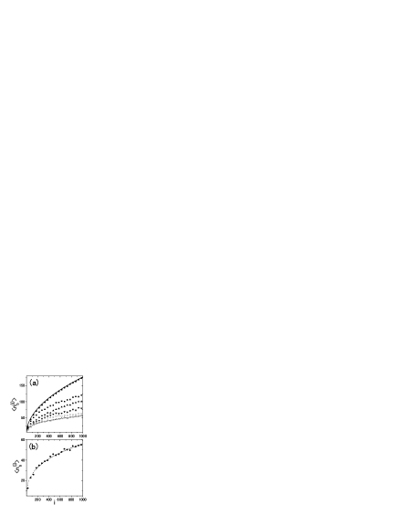
FIG. 12.: (a) Average of $n_{b}^{(i)}$ for $k=0.0$, 0.1, 0.2, 0.3, 0.4, and 0.5 from top to bottom. Averaging is performed as in the previous figure. Solid and dashed lines correspond to $\tau(i)\simeq 5.6i^{1/2}$ and $5.6i^{1/3}$, respectively. (b) Average of $n_{b}^{(i)}$ for $k=0.6$. The dashed line corresponds to $5.6i^{1/3}$.

Now we calculate $n_{b}^{(i)}$ for the present model, Eq. (2), by integrating $\rho$ along the boundary $V(x,y)=E_{i}$. As the potential is homogeneous, $n_{b}^{(i)}$ can be written as,

$$n_{b}^{(i)}=\gamma\oint_{V=E_{i}}ds|{\rm grad}V|^{1/3}=\gamma bE_{i}^{1/2},$$ (33)

with the coefficient $b$ given by

$$b=\oint_{V=1}ds|{\rm grad}V|^{1/3},$$ (34)

where the integral is performed along the curve $V(x,y)=1$. By using the semiclassical relation between the energy $E_{i}$ and the level number $i$ given in Eq. (16), we obtain the level number dependence of the number of intersections:

$$n_{b}^{(i)}=\frac{\gamma b}{N(1)^{1/3}}i^{\prime 1/3}\simeq 3.0i^{\prime 1/3}=4.8i^{1/3},$$ (35)

where $i^{\prime}$ represents the corrected level number and the numerical value $b\simeq 15.26$ evaluated at $k=0.6$ was used.

We note that $n_{b}^{(i)}$ has a $\sqrt{i}$ dependence at $k=0.0$. This indicates that the level number dependence of the number of intersections changes from $i^{1/2}$ to $i^{1/3}$ as the dynamics changes from integrable to chaotic. Numerical results shown in Fig. 12 confirm this. Here, the average value of $n_{b}^{(i)}$ (over 50 levels) is shown as a function of the level number $i$. At $k=0.0$ $n_{b}^{(i)}$ follows well the semiclassical result for the number of intersections shown by the higher curve in Fig. 12(a), i.e.,

$$\tau(i)=\frac{8\pi^{5/4}}{5\sqrt{3}\Gamma(\frac{3}{4})^{2}\Gamma(\frac{5}{4})}\sqrt{i^{\prime}}\simeq 2.8\sqrt{i^{\prime}}=5.6\sqrt{i},$$ (36)

a derivation of which is presented in Appendix C 2. As $k$ increases, $n_{b}^{(i)}$ gradually decreases. Finally, at $k=0.6$, $n_{b}^{(i)}$ follows the curve $5.6i^{1/3}$ shown as the dashed line in Fig. 12 (b), where the fitted value is used as a coefficient. The fitted value 5.6 is a little larger than the predicted value 4.8. This discrepancy may be due to the curvature of the boundary $V(x,y)=1$, which is not taken into account in Eq.(32).

V Distribution of the Area of the Nodal Domains

Let us now consider the distribution of the area of nodal domains. The area distribution may provide a measure as to whether the percolation-like model can be applied. The appropriate length unit to define the area should be the wave length [5] which depends on the energy of the level. Moreover, in contrast to the billiard problem, the wavelength in the present model depend locally on the coordinate due to the presence of the potential $V(x,y)$. We define the scaled area $s$ of the nodal domain for the level $i$ with energy $E_{i}$ by

$$s=\mu\int_{\rm n.d.}(E_{i}-V(x,y))dxdy,$$ (37)

where the integral is performed over each region of the nodal domain. We take the scale factor $\mu=1$. One may note that the parameter $\alpha$ is absent in the definition (37) so that it does not directly influence the properties of the area distribution. The normalized number of nodal domains with area $s$ is defined as [5],

$$n(s)\equiv\sum_{i}\frac{Q_{i}(s)}{i}.$$ (38)

Here, $Q_{i}(s)$ represents the number of nodal domains with area $s$ in the $i$th wave function.

Figure 13 shows the distribution of $n(s)$. The line in the figure represents the power distribution with the Fisher exponent, $n^{\rm F}(s)\propto s^{-\tau}$, where $\tau=187/91$, which we call hereafter the Fisher line. This represents the characteristic distribution at the critical point in the two-dimensional percolation model. The figure shows that the distribution at small values of $k$ deviates considerably from the Fisher line, especially in the small area region. The deviation gradually diminishes as the value of $k$ increases, and at $k=0.6$, the distribution almost coincides with the Fisher line except for a small discrepancy in the small $s$ region. We now study if the latter discrepancy may imply that the assumption behind the percolation-like model does not hold completely even at $k=0.6$.

FIG. 13.: Distribution $n(s)$ for $k=0.0$, 0.1, 0.2, 0.3, 0.4, 0.5, and 0.6 from top to bottom. The values of $n(s)$ are multiplied by a factor $10^{12}$ for $k=0.0$, $10^{10}$ for $k=0.1$, $10^{8}$ for $k=0.2$, $10^{6}$ for $k=0.3$, $10^{4}$ for $k=0.4$, and $10^{2}$ for $k=0.5$. Levels $200\leq i\leq 1000$ are considered. Solid lines show the Fisher line.

We note that the Fisher line was obtained for an infinite lattice of mesh points, while in our finite system the effect of boundary may influence considerably the area distributions. In order to compare with the infinite system and to test the applicability of the percolation model, we have to exclude the effect of the boundary. To this end, it is appropriate to employ only the inner nodal domains to obtain the area distribution.

Figure 14 shows the area distribution $n(s)$ for inner nodal domains. Large deviation from the Fisher line at small $k$ values reflects the fact that the avoided crossings are correlated and the nodal structure does not belong to the universality class of the percolation model. On the other hand, when $k\geq 0.4$, the agreement is very good. Thus we may conclude that the small deviation seen in Fig. 13 at $k\geq 0.4$ is due to the boundary effect.

FIG. 14.: Same as Fig. 13 but for the inner nodal domains. The Fisher line corresponding to $k=0.0$ is omitted.

Remember that the distribution of the number of nodal domains in Fig. 3 and the number of inner nodal domains in Fig. 8 still show a gradual change after $k=0.4$. The area distribution is contrasted to this behavior. The agreement with the Fisher line already at $k\geq 0.4$ may imply that the independence and the randomness of the avoided crossings is practically already realized before the system becomes completely chaotic at $k=0.6$ as given by the classical phase space structure or by the level statistics.

VI Summary

We investigated the transition from integrable to chaotic dynamics from the point of view of the nodal structure in the wave functions by employing a two dimensional quartic oscillator. The distribution of the number of nodal domains, the number of intersections of nodal lines with the boundary of the classically allowed region, and the area distribution of nodal domains were studied as a function of the parameter $k$ which controls the nonintegrability of the system.

The number of nodal domains is drastically reduced as the dynamics of the system changes from integrable ($k=0.0$) to nonintegrable ($k$ nonzero), and then gradually increases as the system becomes chaotic ($k\sim 0.6$). Separation into ‘inner’ and ‘boundary’ nodal domains shows that the above dependence on $k$ mainly comes from the behavior of the former. Perturbative argument suggests that a finite (but small) $k$ gives rise to correlated avoided crossings of nodal lines, leading to a drastic reduction of inner nodal domains. Their number turns to increase again as $k$ becomes larger, which may be related to the loss of the correlations in avoided crossings which underlies the percolation model. The ‘boundary’ nodal domains show, in contrast, a milder dependence on $k$, and its significance in the total number of nodal domains becomes small at large $k$ values. A semiclassical model which incorporates the degree of amplitude mixing as well as properties of avoided crossings has been proposed to study the number of nodal domains.

We studied the distribution of the number of intersections with the boundary of the classically allowed region. We found that the average number shows a different dependence on the level number as the dynamics changes from integrable to chaotic. It is interesting to find such a characteristic connection to the dynamics in the structure of the wave function at the boundary, in view of the rather mild $k$ dependence found in the number of boundary nodal domains.

We studied also the distribution of the nodal domain areas which shows a scaling behavior in the percolation-like model[5]. In the present model, too, the area distribution shows a scaling with the same exponent for large $k$ values. A small deviation has been shown to come from the boundary effect. The scaling behavior seems to be complete before the dynamics reaches the chaotic limit, however.

This raises the question as to how the various signatures on the chaotic properties which appear in the level statistics or in the wave functions are interrelated. Further studies on the typical values of $k$ which characterize the onset or the completion of various structures in the wave functions would be interesting. They include, for instance, the signals studied in the nodal domain distribution, amplitude mixing (Porter-Thomas distribution), loss of correlations in the avoided crossings, scaling in the area distribution, etc. These are left for the future investigation. In this context, it is valuable to mention that even for the superposition of random waves, there is a weak long range correlation among the avoided crossings as discussed in Ref. [14].

A No nodal domain in the classically forbidden region

We prove that there is no nodal domain which is embedded entirely in a classically forbidden region.

Assume that there is such a nodal domain whose region is $D$ for an eigenfunction $\Psi$ (taken real, for simplicity). The eigenfunction $\Psi$ satisfies the following Schrödinger equation;

$$\Delta\Psi=2(V-E)\Psi,$$ (A1)

where $E$ represents the eigenvalue and $V$ the potential. Multiply $\Psi$ on both sides in Eq. (A1) and integrate them over the region $D$. The right hand side becomes positive,

$$2\int_{D}(V-E)\Psi^{2}dv>0,$$ (A2)

because in the classically forbidden region the inequality $V-E>0$ always holds. On the other hand, since the value of $\Psi$ along the boundary of the region $D$ is zero, the left hand side after partial integration becomes

$$\int_{D}\Psi\Delta\Psi dv=-\int_{D}(\nabla\Psi)^{2}dv<0,$$ (A3)

which is in contradiction to Eq. (A2). Therefore there is no nodal domain in the classically forbidden region.

B Number of nodal domains for a given diagram of nodal lines

We derive the relation (3) for the number of nodal domains in a two-dimensional area enclosed by a boundary $B$. See also Ref. [11] for a slightly different form of the relation for the number of nodal domains expressed in terms of the number of nodal lines, etc. The nodal lines and the boundary represent a kind of a diagram in a two-dimensional plane which is constructed with a number of vertices (nodal crossings including nodal contacts at the boundary) that are connected with edges, i.e., the line segments of nodal lines or those of the boundary. We first consider a general diagram made of nodal lines and then restrict it to the special case treated in the text.

Let us define the degree $k$($\geq 3$) of a vertex as the number of lines which are connected at the vertex. We define also ‘island’ (in $B$) as the cluster of nodal lines which are linked neither to $B$ nor to the other clusters of nodal lines. Simplest island is a ‘bubble’, i.e., a closed line without a vertex. For instance, a bubble within a bubble will make two islands.

We now consider the number $N$ of nodal domains for a diagram of nodal lines in $B$ with $m$ islands, where the total number of vertices of degree $k$($\geq 3$) is $n_{k}$. Since there are $m+1$ clusters of nodal lines disconnected from each other, we assign them an index $j=0,1,\cdots,m$, where $j=0$ denotes the cluster which involves the boundary $B$, while $j=1,\cdots,m$ denote islands. For each cluster $j$ we assign the number of nodal domains $N_{j}$, the total number of edges $e_{j}$, and that of vertices $v_{j}$ which is given by the sum of $n_{k}(j)$, the number of vertices with degree $k$ in the $j$-th cluster. If we neglect the case of ‘bubbles’ for a moment, we can use Euler’s formula for each cluster $j$ to obtain

$$N_{j}+1=e_{j}-v_{j}+2,\qquad(j=0,1,2,\ldots,m)$$ (B1)

where we added unity on the left hand side, since $N_{j}$ counts domains only inside the boundary. By using the graphical relation

$$e_{j}=\frac{1}{2}\sum_{k\geq 3}k\,n_{k}(j),$$ (B2)

the relation (B1) is transformed to

$$N_{j}=\sum_{k\geq 3}\left(\frac{1}{2}k-1\right)n_{k}(j)+1.$$ (B3)

Equation (B3) is seen to hold also for a ‘bubble’, where $N=1$ and all $n_{k}$’s are zero. By summing up over $j$ we obtain the relation

$$N=\sum_{j=0}^{m}N_{j}=\sum_{k\geq 3}\left(\frac{1}{2}k-1\right)n_{k}+m+1,$$ (B4)

where we used $n_{k}=\sum_{j}n_{k}(j)$.

In the special case treated in Sec. III, we assumed that there are no accidental crossing of more than two nodal lines at a point inside $B$, and also that no accidental contact of more than one nodal line on $B$. In this case, the vertex inside $B$ has a degree 4, and the vertex on $B$ has a degree 3. Thus the number of nodal domains $N(b,c,m)$ for a diagram with $c(=n_{4})$ crossings, $b(=n_{3})$ points of contact on $B$, and $m$ islands is given by

$$N(b,c,m)=\frac{1}{2}b+c+m+1,$$ (B5)

which is the relation (3).

C Derivation of some relations

We give brief derivations for Eqs. (8) and (36). See Sec. III D for notations.

1 A derivation of Eq. (8)

For the wave function $\psi_{n1}(x,y)$ which has corresponding actions, $I_{1}=I$, $I_{2}=0$, the semiclassical number of nodal domains $N_{i}$ can be written as,

$$N_{i}=I=g(E),$$ (C1)

while the semiclassical level number is given by Eq. (16). Then, the coefficient $d$ in Eq. (8) is given by

$$d=1/\sqrt{N(1)},$$ (C2)

which leads to Eq. (8) for the quartic oscillator model.

2 A derivation of Eq. (36)

Analogous to Eq. (12), the distribution function of $n_{b}^{(i)}/\sqrt{i}$ can be written as,

$$P(\eta)=\frac{1}{N_{A}}\int_{I_{1},I_{2}\in A}dI_{1}dI_{2}\delta\left(\eta-\frac{\tau(I_{1},I_{2})}{\sqrt{N(E)}}\right),$$ (C3)

where $\tau(I_{1},I_{2})=2(I_{1}+I_{2})$ is the number of nodal intersections. By the same variable transformation as in Sec. III D and by performing the integration over the variable $E$, the average of $\eta$ can be written as,

$$\langle\eta\rangle=\frac{2}{N(1)^{3/2}}\int_{\Gamma}drL(r)(I_{1}^{(0)}(r)+I_{2}^{(0)}(r)).$$ (C4)

Inserting Eq. (15) and transforming the variable $r$ to $I_{1}^{(0)}(=x)$, the integral in Eq. (C4) can be expressed as,

$$\int_{0}^{1}dxx(1-x^{\ell})^{\frac{1}{\ell}}+\int_{0}^{1}dx(1-x^{\ell})^{\frac{2}{\ell}}$$ (C5)

$$=\frac{\Gamma\left(\frac{2}{\ell}\right)\Gamma\left(\frac{\ell+1}{\ell}\right)}{\ell\Gamma\left(\frac{\ell+3}{\ell}\right)}+\frac{\Gamma\left(\frac{1}{\ell}\right)\Gamma\left(\frac{\ell+2}{\ell}\right)}{\ell\Gamma\left(\frac{\ell+3}{\ell}\right)},$$ (C6)

for the Hamiltonian with the form Eq. (25). Thus, for the quartic oscillator model ($\ell=4/3$), Eq. (C4) gives the coefficient in Eq. (36).

D Example for the calculation of the average of nodal domain numbers

We here show the increase of average of $N_{i}/i$ after $\omega\geq\frac{1}{2}r_{\rm max}$ by using Eq. (22) with the assumption that the reduction factor $G$ can be obtained from the percolation model. The reduction factor $G(I_{1},I_{2})$ may still have a dependence on $I_{1}$ and $I_{2}$, however, when the energy is not so high.

As for the smoothing function, we adopt the following form:

$$f_{\omega}(r,r^{\prime})={\theta(\omega-|r-r^{\prime}|)\over\min(r+\omega,r_{\rm max})-\max(r-\omega,0)}.$$ (D1)

The average of $N_{i}/i$ can be written as,

$$\left\langle{N_{i}\over i}\right\rangle={1\over N_{A}}\int_{E_{1}}^{E_{2}}J(E)dE\int_{\Gamma}drL(r)$$ (D2)

$$\times{I^{(0)}_{1}(r_{\omega})I^{(0)}_{2}(r_{\omega})\over N(1)}G(I^{(0)}_{1}(r_{\omega})g,I^{(0)}_{1}(r_{\omega})g),$$ (D3)

where $r_{\omega}=r_{\omega}(r)$ and $g=g(E)$. We differentiate Eq. (D3) with respect to $\omega$,

$$\frac{d}{d\omega}\left\langle{N_{i}\over i}\right\rangle={1\over N_{A}}\int_{E_{1}}^{E_{2}}J(E)dE\int_{\Gamma}drL(r)$$ (D4)

$$\times{r_{\omega}^{\prime}\over N(1)}C(E,r)$$ (D5)

$$C(E,r)=(I_{1}^{(0)\prime}(r_{\omega})I_{2}^{(0)}(r_{\omega})+I_{1}^{(0)}(r_{\omega})I_{2}^{(0)\prime}(r_{\omega}))G$$ (D6)

$$+I_{1}^{(0)}(r_{\omega})I_{2}^{(0)}(r_{\omega})g({\partial G\over\partial a}I_{1}^{(0)\prime}+{\partial G\over\partial b}I_{2}^{(0)\prime}),$$ (D7)

where $r_{\omega}^{\prime}=dr_{\omega}(r)/d\omega$, $I_{1}^{(0)\prime}(r)=dI_{1}^{(0)}(r)/dr$, and $\partial G/\partial a=\partial G(a,b)/\partial a$ etc.

When $\omega>\frac{1}{2}r_{\rm max}$, the function $r_{\omega}^{\prime}$ has a following form;

$$r_{\omega}^{\prime}(r)=\left\{\begin{array}[]{rl}{1\over 2},&\quad(r\leq r_{\rm max}-\omega)\\ 0,&\quad(r_{\rm max}-\omega<r\leq\omega)\\ -{1\over 2},&\quad(r>\omega).\end{array}\right.$$ (D8)

Accordingly, the integration range of $r$ in Eq. (D5) is restricted to $(0,r_{\rm max}-\omega)$ and $(\omega,r_{\rm max})$. By using the relation $G(a,b)=G(b,a)$ and approximate relations $I^{(0)}_{1}(r)=I^{(0)}_{2}(r_{\rm max}-r)$ and $I^{(0)\prime}_{1}(r)=-I^{(0)\prime}_{2}(r_{\rm max}-r)$, the latter integration range can be transformed to the former as,

$$\frac{d}{d\omega}\left\langle{N_{i}\over i}\right\rangle={1\over N_{A}N(1)}\int_{E_{1}}^{E_{2}}J(E)dE$$ (D9)

$$\times\int_{0}^{r_{\rm max}-\omega}drL(r)C(E,r).$$ (D10)

Above approximate relations are justified by an approximate symmetry between the variables $I_{1}$ and $I_{2}$, because the symmetry breaking in the Hamiltonian (2) is small. The behavior of the average is, thus, determined by the function $C(E,r)$. The function $C(E,r)$ can be written as,

$$C(E,r)=I^{(0)\prime}_{1}I^{(0)}_{2}\Biggl{\{}\left(1+{I^{(0)}_{1}\over I^{(0)}_{2}}{dI^{(0)}_{2}\over dI^{(0)}_{1}}\right)G$$ (D11)

$$+I^{(0)}_{1}g\left({\partial G\over\partial a}+{dI^{(0)}_{2}\over dI^{(0)}_{1}}{\partial G\over\partial b}\right)\Biggr{\}}.$$ (D12)

Since the range of $r_{\omega}$ is $\frac{1}{4}r_{\rm max}\leq r_{\omega}\leq\frac{1}{2}r_{\rm max}$ for $\omega\geq\frac{1}{2}r_{\rm max}$, where the boundary effect is negligible, the value of the reduction factor $G$ will be close to the asymptotic one. Thus, the derivative of $G$ is near zero;

$${\partial\over\partial a}G(a,b)={\partial\over\partial b}G(a,b)\simeq 0.$$ (D13)

Accordingly, the second term in Eq. (D12) is neglected. We also assume the Hamiltonian for integrable case has the form, Eq. (25). The function $C(E,r)$ ,then, can be approximately written as,

$$C(E,r)\simeq I^{(0)\prime}_{1}I^{(0)}_{2}\left(1-\left({I^{(0)}_{1}\over I^{(0)}_{2}}\right)^{\ell}\right)G.$$ (D14)

Since in the considered range of $r_{\omega}$, the relation $I^{(0)}_{1}\leq I^{(0)}_{2}$ always holds, the derivative of average with respect to $\omega$ is positive,

$$\frac{d}{d\omega}\left\langle{N_{i}\over i}\right\rangle\geq 0.$$ (D15)

This result shows that the average of $N_{i}/i$ increases as the smoothing width $\omega$, as long as $\omega\geq\frac{1}{2}r_{\rm max}$. The increase of the average stops when the condition $I^{(0)}_{1}=I^{(0)}_{2}$ always holds, which means $r_{\omega}=\frac{1}{2}r_{\rm max}$, namely the chaotic limit.

REFERENCES

- [1] M.V. Berry, J. Phys. A 10, 2083(1977).
- [2] S.W. McDonald and A N. Kaufman, Phys. Rev. Lett. 42, 1189 (1979).
- [3] T.A. Brody, et al., Rev. Mod. Phys. 53, 385 (1981).
- [4] G. Blum, S. Gnutzmann, and U. Smilansky, Phys. Rev. Lett. 88, 114101 (2002).
- [5] E. Bogomolny and C. Schmit, Phys. Rev. Lett. 88, 114102 (2002).
- [6] N. Savytskyy, O. Hul, and L. Sirko, Phys. Rev. E 70, 056209 (2004).
- [7] See, for instance, H.-D. Mayer, J. Chem. Phys. 84, 3147 (1986).
- [8] Th. Zimmermann, H.-D. Meyer, H. Koppel, and L. S. Cederbaum, Phys. Rev. A 33, 4334 (1986).
- [9] J. Hoshen and R. Kopelman, Phys. Rev. B 14, 3438 (1976).
- [10] H. Aiba and T. Suzuki, Phys. Rev. E 63, 026207 (2001).
- [11] T. Hoffmann-Ostenhof, P. Michor, and N. Nadirashvili, Geom. Funct. Anal. 9, 1169 (1999); N. Nadirashvili, Math. USSR Sbornik 61, 225 (1988).
- [12] A. G. Monastra, U. Smilansky, and S. Gnutzmann, J. Phys. A 36, 1845 (2003).
- [13] W. E. Bies and E. J. Heller, J. Phys. A 35, 5673 (2002).
- [14] G. Foltin, S. Gnutzmann, and U. Smilansky, J. Phys. A 37, 11363 (2004).