Asymptotic properties of mathematical models of excitability

Abstract

singular perturbations, action potential, front dissipation We analyse small parameters in selected models of biological excitability, including Hodgkin-Huxley (1952) model of nerve axon, Noble (1962) model of heart Purkinje fibres, and Courtemanche et al. (1998) model of human atrial cells. Some of the small parameters are responsible for differences in the characteristic timescales of dynamic variables, as in the traditional singular perturbation approaches. Others appear in a way which makes the standard approaches inapplicable. We apply this analysis to study the behaviour of fronts of excitation waves in spatially-extended cardiac models. Suppressing the excitability of the tissue leads to a decrease in the propagation speed, but only to a certain limit; further suppression blocks active propagation and leads to a passive diffusive spread of voltage. Such a dissipation may happen if a front propagates into a tissue recovering after a previous wave, e.g. re-entry. A dissipated front does not recover even when the excitability restores. This has no analogy in FitzHugh-Nagumo model and its variants, where fronts can stop and then start again. In two spatial dimensions, dissipation accounts for break-ups and self-termination of re-entrant waves in excitable media with Courtemanche et al. (1998) kinetics.

1 Introduction

The motivation of this study comes from a series of numerical simulations of spiral waves [Biktasheva-etal-2003] in a model of human atrial tissue based on the excitation kinetics of Courtemanche-etal-1998 (CRN). The spiral waves in this model tend to break up into pieces and even spontaneously self-terminate (see fig. 1).

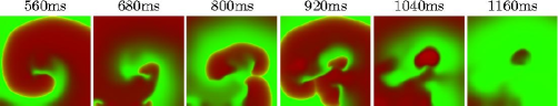
Figure 1: Self-termination of a spiral wave in the CRN model. Red colour component: transmembrane voltage $E$, green colour component: gating variable $o_{i}$. Diffusion coefficient $D=0.03125\mathrm{mm}^{2}/\mathrm{ms}$, preparation size $75\times 75\,\mathrm{mm}$. See also [Biktasheva-etal-2003].

No mathematical model of cardiac tissue is now considered ultimate or can claim absolute predictive power. The spontaneous self-termination may be relevant to human atrial tissue or may be an artefact of modelling. Understanding the mechanism of this behaviour in some simple terms would allow a more direct and certain verification. This is difficult as the models are very complex and the events depicted in fig. 1 have many different aspects. Traditionally, such understanding has been achieved in terms of simplified models, starting from axiomatic cellular automata description [Wiener-Rosenblueth-1946] through to simplified PDE models [FitzHugh-1961, Nagumo-etal-1962] which allow asymptotic study by means of singular perturbation techniques [Tyson-Keener-1988]. This approach can describe some of the features observed in fig. 1, e.g. the “APD restitution slope 1” theory predicts when the stationary rotation of a spiral wave is unstable against alternans [Nolasco-Dahlen-1968, Karma-etal-1994, Karma-1994]. The relevance of the “slope-1” theory to particular models is debated [Cherry-Fenton-2004], but in any case it only predicts the instability of a spiral wave, not whether it will lead to complete self-termination of the spiral wave, its breakup, or just meandering of its tip. We need to understand how the propagation of a wave is blocked. This has unexpectedly turned out to be rather interesting. Some features of the propagation block in fig. 1 can never be explained within the standard FitzHugh-Nagumo approach. As this was the only well developed asymptotic approach to excitable systems around, we had either to accept that this problem is too complicated to be understood in simplified terms, or to develop an alternative type of simplified model and corresponding asymptotics.

We chose the latter. This paper summarizes our progress in this direction in the last few years [Biktashev-2002, Biktashev-2003, Biktasheva-etal-2003, Suckley-Biktashev-2003, Biktashev-Suckley-2004, Suckley-2004, Biktashev-Biktasheva-2005]. The results on the asymptotic structure of the CRN model are published for the first time.

2 Tikhonov asymptotics

The standard Tikhonov-Pontryagin singular perturbation theory [Tikhonov-1952, Pontryagin-1957] summarized in [Arnold-etal-1994] is usually formulated in terms of “fast-slow” systems in one of the two equivalent forms

$$\begin{array}[]{l}{\mathrm{d}\mathbf{X}}/{\mathrm{d}t}=\mathbf{f}(\mathbf{X},\mathbf{Y})\\ \epsilon{\mathrm{d}\mathbf{Y}}/{\mathrm{d}t}=\mathbf{g}(\mathbf{X},\mathbf{Y})\end{array}\Leftrightarrow\begin{array}[]{l}{\mathrm{d}\mathbf{X}}/{\mathrm{d}T}=\epsilon\mathbf{f}(\mathbf{X},\mathbf{Y})\\ {\mathrm{d}\mathbf{Y}}/{\mathrm{d}T}=\mathbf{g}(\mathbf{X},\mathbf{Y})\end{array}$$ (1)

where $\epsilon>0$ is small, $t$ is the “slow time”, $T$ is the “fast time”, $t=\epsilon T$, $\mathbf{X}$ is the vector of “slow variables” and $\mathbf{Y}$ is the vector of “fast variables”. The theory is applicable if all relevant attractors of the fast subsystem are asymptotically stable fixed points. So the variables have to be explicitly classified as fast and slow, and the system should contain a small parameter which formally tends to zero although the original system is formulated for a particular value of that parameter, say 1.

We consider Hodgkin-Huxley-1952 (henceforth referred to as HH) and Noble-1962 (henceforth N62) models. Both can be written in the same form,

$${\mathrm{d}E}/{\mathrm{d}t} = -{\Sigma_{I}}(E,h,m,n)/C_{M},$$

$${\mathrm{d}y}/{\mathrm{d}t} = {(\overline{y}(E)-y)}/{\tau_{y}(E)},\quad y=m,h,n,$$ (2)

where ${\Sigma_{I}}(E,h,m,n)=(g_{K}n^{4}+g_{K_{1}}(E))(E-E_{K})+(g_{Na}m^{3}h+g_{Na_{1}})(E-E_{Na})+g_{l}(E-E_{l})$ is the total transmembrane current ($\mu\mathrm{A}/\mathrm{cm}^{2}$), $t$ is time ($\mathrm{ms}$), $E$ is the transmembrane voltage ($\mathrm{mV}$), $E_{k}$, $k=Na,K,l$ are the reversal potentials of sodium, potassium and leakage currents respectively ($\mathrm{mV}$), $\bar{g}_{k}$ are the corresponding maximal specific conductances ($\mathrm{mS}/\mathrm{cm}^{2}$), $n$, $m$, $h$ are dimensionless “gating” variables, $C_{M}$ is the specific membrane capacitance ($\mu\mathrm{F}/\mathrm{cm}^{2}$), $\overline{y}(E)$ are the gates’ instantaneous equilibrium “quasi-stationary” values, and $\tau_{y}(E)$ are the characteristic timescale coefficients of the gates dynamics ($\mathrm{ms}$). Definition and comparison of parameters and functions used in (2) for HH and N62 models can be found in [Suckley-Biktashev-2003].

To classify the dynamic variables by their speeds, we define empiric characteristic timescale coefficients, $\tau_{i}$. For a system of differential equations ${\mathrm{d}x_{i}}/{\mathrm{d}t}=f_{i}(x_{1},\dots,x_{N})$, $i=1,\dots,N$, we define $\tau_{i}(x_{1},\dots,x_{N})\equiv\left|\left({\partial f_{i}}/{\partial x_{i}}\right)^{-1}\right|$. The $\tau$’s obtained for $m$, $h$ and $n$ in this way coincide with $\tau_{m,h,n}$ in (2), and this definition can be extended to other variables, e.g. $E$ in the case of (2).

Hodgkin-Huxley.

Fig. 2(a) shows how $\tau$’s change during a typical action potential (AP) in the HH model. The speeds of $E$ and $m$ exchange places during the AP, as do the speeds of $h$ and $n$, but at all times the pair $(E,m)$ remains faster than the pair $(h,n)$. This suggests introduction into system (2) of a parameter $\epsilon$ which in the limit $\epsilon\rightarrow 0$ makes variables $E$ and $m$ much faster than $n$ and $h$:

$$\epsilon{\mathrm{d}m}/{\mathrm{d}t} = {(\overline{m}(E)-m)}/{\tau_{m}(E)},$$

$$\epsilon{\mathrm{d}E}/{\mathrm{d}t} = -{\Sigma_{I}}(E,h,m,n)/C_{M},$$

$${\mathrm{d}h}/{\mathrm{d}t} = {(\overline{h}(E)-h)}/{\tau_{h}(E)},$$

$${\mathrm{d}n}/{\mathrm{d}t} = {(\overline{n}(E)-n)}/{\tau_{n}(E)}.$$ (3)

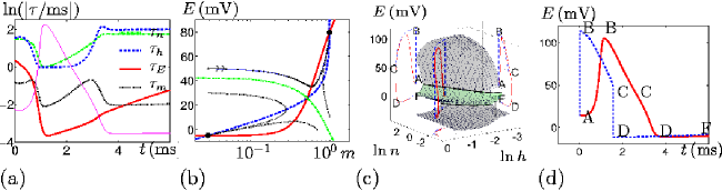
Figure 2: Tikhonov asymptotics of HH. (a) Characteristic times $\tau_{i}$ during an AP. Thin solid magenta line: the AP for a reference. (b) Phase portrait of the fast subsystem (4) at $n=0.37$, $h=0.02$. Solid red line: horizontal isocline. Dashed blue line: vertical isocline. Filled black circles: stable equilibria. Dash-dotted green line: stable separatrix of the saddle, the boundary of attraction basins. Black dotted lines: selected trajectories. (c) A three-dimensional view of the slow manifold (the surface). Solid line: the fold line. Dotted line: the selected trajectory and its projections on coordinate walls. (d) AP in the original model, $\epsilon=1$, solid red line, and when the fast variables are made faster, $\epsilon=10^{-3}$, dashed blue line. See also [Suckley-Biktashev-2003].

The properties of this system in the limit $\epsilon\rightarrow 0$ are shown in fig. 2(b–c). The fast transient, corresponding to the AP upstroke can be studied by changing the independent time variable in (3) to $T=t/\epsilon$ and then considering the limit $\epsilon\rightarrow 0$ which gives the fast subsystem of two equations for $m$ and $E$,

$${\mathrm{d}m}/{\mathrm{d}T} = {(\overline{m}(E)-m)}/{\tau_{m}(E)},$$

$${\mathrm{d}E}/{\mathrm{d}T} = -{\Sigma_{I}}(E,h,m,n)/C_{M},$$ (4)

in which the slow variables $h$ and $n$ are parameters as their variations during the onset are negligible. An example of a phase portrait of system (4) at selected values of $h$ and $n$ is shown in fig. 2(b). It is bistable, i.e it has two asymptotically stable equilibria, and a particular trajectory approaches one or the other depending on the initial conditions. The basins of attraction of the two equilibria are separated by the stable separatrices of a saddle point, which is the threshold between “all” and “none” responses. A fine adjustment of initial conditions at the threshold will cause the system to come to the saddle point. This is a mathematical representation of the excitation threshold in Tikhonov asymptotics.

For different values of $n$ and $h$, the location of the equilibria in the fast subsystem vary. All equilibria $(E,m)$ at all values of $n$ and $h$ form a two-dimensional slow manifold in the four-dimensional phase space of (3) with coordinates $(E,m,h,n)$. Projection of this two-dimensional manifold into the three dimensional space with coordinates $(E,h,n)$ is depicted in fig. 2(c). It has a characteristic cubic folded shape, with two fragments of a positive slope (as it appears on the figure), separated by an “overhanging” fragment of a negative slope. The borders between the fragments are the fold lines, seen as nearly horizontal solid curves on the picture. The positive slope fragments consist of stable equilibria, and the negative slope fragment consists of unstable equilibria (saddle points) of the fast subsystem.

The points of this manifold are steady-states if considered on the time scale $T\sim 1$ or equivalently $t\sim\epsilon$. On the time scale $t\sim 1$ these points are no longer steady states, but we observe a slow (compared to the initial transient) movement along this manifold, which explains its name. Asymptotically, the evolution on the scale $t\sim 1$ can be described by the limit $\epsilon\rightarrow 0$ in (3), which gives a system of two finite equations and two differential equations,

$$0 = {\overline{m}(E)-m},$$

$$0 = {\Sigma_{I}}(E,h,m,n),$$

$${\mathrm{d}h}/{\mathrm{d}t} = {(\overline{h}(E)-h)}/{\tau_{h}(E)},$$

$${\mathrm{d}n}/{\mathrm{d}t} = {(\overline{n}(E)-n)}/{\tau_{n}(E)},$$ (5)

The finite equations define the slow manifold and the differential equations define the movement along it.

Fig. 2(c) shows a selected trajectory of system (3) corresponding to a typical AP solution. The only equilibrium of the full system (3), corresponding to the resting state, is at the lower, “diastolic” branch of the slow manifold. If the initial condition is in the basin of the upper branch, the trajectory starts with a fast initial transient, corresponding to the upstroke of the AP, then proceeds along the upper, “systolic” branch of the slow manifold, which corresponds to the plateau of the AP. When the trajectory reaches the fold line, a boundary of the systolic branch, the plateau stage is over. The fast subsystem is no longer bistable. The only stable equilibrium is now at the diastolic branch. So the trajectory jumps down. This is repolarization from the AP and it happens at the time scale $t\sim\epsilon$. The trajectory then slowly proceeds along the diastolic branch towards the resting state.

So, an inevitable feature of the asymptotics (3) is that the solution at smaller $\epsilon$ has not only a faster upstroke, but also a faster repolarization, and the asymptotic limit of the AP shape is rectangular as opposed to the triangular shape in the exact model, see fig. 2(d). This is undesirable as it means that asymptotic formulae obtained in this way produce qualitatively inappropriate results.

The practical importance of this excercise is limited as in HH the AP are not much longer than upstrokes.

Noble 1962.

This model is more relevant to cardiac AP. The speed analysis of N62 model, similar to the one we have done for HH model, reveals a different asymptotic structure but ultimately similar results. Fig. 3(a) demonstrates three rather than two different time scales. Variable $m$ is the fastest of all, we call it “superfast”. Of the remaining three, variables $E$ and $h$ are fast and variable $n$ is slow. So we need two small parameters, $\epsilon_{1}$ to describe the difference between the fast and superfast time scales, and $\epsilon_{2}$ to describe the difference between the slow and fast time scales. System (2) then takes the form

$$\epsilon_{2}\epsilon_{1}{\mathrm{d}m}/{\mathrm{d}t} = {(\overline{m}(E)-m)}/{\tau_{m}(E)},$$

$$\epsilon_{2}{\mathrm{d}E}/{\mathrm{d}t} = -{\Sigma_{I}}(E,h,m,n)/C_{M},$$

$$\epsilon_{2}{\mathrm{d}h}/{\mathrm{d}t} = {(\overline{h}(E)-h)}/{\tau_{h}(E)},$$

$${\mathrm{d}n}/{\mathrm{d}t} = {(\overline{n}(E)-n)}/{\tau_{n}(E)}.$$ (6)

Consider first the limit $\epsilon_{1}\rightarrow 0$. The superfast subsystem consists of one differential equation for $m$. It always has exactly one equilibrium which is always stable. So after a supershort transient, $m(t)$ is always close to its quasi-stationary value $\overline{m}(E(t))$. Thus, with an error $\sim\epsilon_{1}$ we may approximate $m$ by $\overline{m}$ and discard the first equation, i.e. adiabatically eliminate superfast variable $m$.

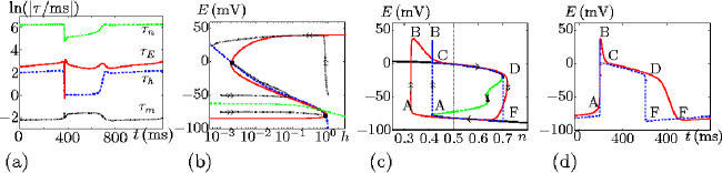
Figure 3: Tikhonov asymptotics of N62. (a,b,d) Notations similar to fig. 2. (c) A two-dimensional view of the stable (black solid) and unstable (green dashed) branches of the slow manifold, and typical pacemaker potential trajectories (the limit cycles): solid red ($\epsilon_{2}=1$) and dashed blue ($\epsilon_{2}=10^{-3}$), vertical dash-dotted line shows value $n=0.5$ for the fast phase portrait on (b). See also [Suckley-Biktashev-2003].

With the remaining system of three differential equations for $E$, $h$ and $n$, we consider the change of the time variable as before, $t=\epsilon_{2}T$, and proceed to the limit $\epsilon_{2}\rightarrow 0$. This produces the fast subsystem in the form

$${\mathrm{d}E}/{\mathrm{d}T} = -{\Sigma_{I}}(E,h,\overline{m}(E),n)/C_{M},$$

$${\mathrm{d}h}/{\mathrm{d}T} = (\overline{h}(E)-h)/{\tau_{h}(E)}.$$ (7)

Fig. 3(b) shows a phase portrait of this system for a selected value of $n$ when (7) is bistable. As there is one slow variable, all the equilibria of the fast subsystem form a one-dimensional manifold, i.e. a curve, in the three-dimensional phase space with coordinates $(E,h,n)$. Its projection on the plane $(h,E)$ is shown in fig. 3(c). Again the stable equilibria correspond to one slope (negative for the given choice of coordinates) and the opposite slope corresponds to the unstable equilibria. The branches are separated from each other by fold points. Again we have an upper, systolic branch, separated from the lower, diastolic branch, and the system has no alternative but to jump from one branch to the other in the time scale $t\sim\epsilon_{2}$. As it happens, there are no true equilibria in the N62 model at standard parameter values, so these jumps happen periodically, producing pacemaker potential. This corresponds to the automaticity of cardiac Purkinje cells. Certain physiologically feasible changes of parameters may produce an asymptotically stable equilibrium at the diastolic branch, i.e turn an automatic Purkinje cell into an excitable cell.

The systolic branch is separated from the diastolic branch, so in the asymptotic limit $\epsilon_{2}\rightarrow 0$, if the upstrokes are fast, the repolarizations are similarly fast. This is in contradiction with the behaviour of the full model, which makes such an asymptotic analysis unsuitable.

3 Non-Tikhonov asymptotics

Noble 1962.

To overcome the difficulties of the Tikhonov approach, we have developed an alternative based on actual biophysics behind N62 and other cardiac excitation models, see fig. 4(a). The upstroke of an AP is much faster than the repolarization as the two processes are caused by different ionic currents. The upstroke is very fast as the fast Na current causing it is very large. However all other currents, including the outward K currents that bring about repolarization are not as large, and there is no reason to tie the two classes of currents together in an asymptotic description. Mathematically, this means that in the right-hand side of the equation for $E$, only the term corresponding to the fast Na current is large and should have the coefficient $\epsilon_{2}^{-1}$ in front of it.

Next, the fast Na current is large only during AP upstroke, and remains small during other stages. The current is regulated by two gating variables, $m$ and $h$, and the quasi-stationary value of the specific conductivity of the current, defined as $W(E)=\overline{m}^{3}(E)\overline{h}(E)$, is always much smaller than one. This happens because $m,h\in[0,1]$ and $\overline{m}^{3}(E)$ is very small for $E$ below a certain threshold voltage $E_{m}$, and $\overline{h}(E)$ is very small for $E$ above another threshold voltage $E_{h}$, and $E_{h}<E_{m}$. So the ranges of almost complete closure of $\overline{m}^{3}(E)$ and $\overline{h}(E)$ overlap. So whenever $E$ changes so slow that $m$ and $h$ have enough time to approach their quasi-stationary values, the fast Na channels are mostly closed. The possibility for the opening of a large fraction of Na channels only exists during the fast upstroke, as $m$ gates are much faster than $h$ gates and have time to open before $h$ close.

Thus, the facts that $m$ gate is much faster than $h$ gate, $\overline{m}^{3}(E)\ll 1$ for $E<E_{m}$, $\overline{h}(E)\ll 1$ for $E>E_{h}$ and $E_{h}<E_{m}$, are all related and reveal why the upstroke of the AP is much faster than all other stages.

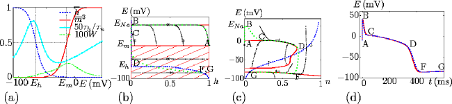
Figure 4: Non-Tikhonov asymptotics of N62, excitable variant. (a) Functions of $E$ illustrating the small quantities taken into account. (b) Phase portrait of the fast subsystem. (c) Phase portrait of the slow subsystem. (d) Action potential solution of (9) for $\epsilon_{2}=1$, solid red, and for $\epsilon_{2}=10^{-3}$, dashed blue. See also [Biktashev-Suckley-2004].

We adopt the hierarchy of times suggested by the formal speed analysis in the previous section, i.e. $m$ is a superfast variable, $E$ and $h$ are equally fast variables and $n$ is a slow variable. We keep the same notation $\epsilon_{1}$ and $\epsilon_{2}$ for the corresponding small parameters. The small parameters should also ensure that $\overline{m}^{3}(E)$ and $\overline{h}(E)$ are small in some ranges of $E$ but not in others. We identify this smallness with $\epsilon_{2}$ rather than $\epsilon_{1}$, as it is to compensate the large value of $g_{Na}$ outside the upstroke, and the large value of $g_{Na}$ is described by $\epsilon_{2}$. We denote the $\epsilon_{2}$-dependent versions of $\overline{m}^{3}(E)$ and $\overline{h}(E)$ as $\hat{{\overline{m}^{3}}}(E;\epsilon_{2})$ and $\hat{{\overline{h}}}(E;\epsilon_{2})$. In this way we obtain

$$\epsilon_{1}\epsilon_{2}{\mathrm{d}m}/{\mathrm{d}t} = {(\hat{{\overline{m}}}(E;\epsilon_{2})-m)}/{\tau_{m}(E)},\qquad\hat{{\overline{m}}}(E;0)=M(E)\theta(E-E_{m}),$$

$$C_{M}{\mathrm{d}E}/{\mathrm{d}t} = \epsilon_{2}^{-1}g_{Na}\left(E_{Na}-E\right)m^{3}h+g_{K}\left(E_{K}-E\right)n^{4}$$

$$+ g_{Na_{1}}(E)\left(E_{Na}-E\right)+g_{K_{1}}(E)\left(E_{K}-E\right)+g_{l}\left(E_{l}-E\right),$$

$$\epsilon_{2}{\mathrm{d}h}/{\mathrm{d}t} = {(\hat{{\overline{h}}}(E;\epsilon_{2})-h)}/{\tau_{h}(E)},\qquad\overline{h}(E;0)=H(E)\theta(E_{h}-E),$$

$${\mathrm{d}n}/{\mathrm{d}t} = {(\overline{n}(E)-n)}/{\tau_{n}(E)},$$ (8)

where $\theta()$ is the Heaviside function.

The limit $\epsilon_{1}\rightarrow 0$ gives adiabatic elimination of the $m$ gate, $m\approx\overline{m}(E)$.

The analysis of the limit $\epsilon_{2}\rightarrow 0$ is complicated by a feature incidental to N62 and not found in other cardiac excitation models. The small conductivity of the window current, $W(E)$, is multiplied by a large factor $g_{Na}$. In N62 the resulting window component of $I_{\mathrm{Na}}$ is comparable to other small currents and cannot be neglected outside the upstroke. The implications of this complication are analysed in [Biktashev-Suckley-2004]. The result, in brief, is that the $\epsilon_{2}$-dependent part of (8) can, in the limit $\epsilon_{2}\rightarrow 0$, be replaced with a “modified N62” model:

$$C_{M}{\mathrm{d}E}/{\mathrm{d}t} = \epsilon_{2}^{-1}g_{Na}\left(E_{Na}-E\right)M^{3}(E)\theta(E-E_{m})h+g_{K}\left(E_{K}-E\right)n^{4}+G(E)$$

$$\epsilon_{2}{\mathrm{d}h}/{\mathrm{d}t} = {(H(E)\theta(E_{h}-E)-h)}/{\tau_{h}(E)},$$

$${\mathrm{d}n}/{\mathrm{d}t} = {(\overline{n}(E)-n)}/{\tau_{n}(E)},$$ (9)

where $G(E)=g_{Na}\left(E_{Na}-E\right)W(E)+g_{Na_{1}}(E)\left(E_{Na}-E\right)+g_{K_{1}}(E)\left(E_{K}-E\right)+g_{l}\left(E_{l}-E\right)$, and as before $M(E)\approx\overline{m}(E)$ for $E>E_{m}$, $H(E)\approx\overline{h}(E)$ for $E<E_{h}$ and $W(E)=\overline{m}^{3}(E)\overline{h}(E)$.

The limit $\epsilon_{2}\rightarrow 0$ of (9) in the fast time $T=t/\epsilon_{2}$ gives the fast subsystem

$$C_{M}{\mathrm{d}E}/{\mathrm{d}T} = g_{Na}\left(E_{Na}-E\right)M^{3}(E)\theta(E-E_{m})h$$

$${\mathrm{d}h}/{\mathrm{d}T} = {(H(E)\theta(E_{h}-E)-h)}/{\tau_{h}(E)}.$$ (10)

As intended, (10) takes into account only the fast sodium current and the gates controlling it, and everything else is a small perturbation on this timescale. The phase portrait of (10) is unusual, see fig. 4(b). The horizontal isocline (the red set) is not just a curve but contains a whole domain $E<E_{m}$. The vertical isocline (the blue set) lies entirely within the red set, so the whole line $h=H(E)\theta(E_{h}-E)$ consists of equilibria. An upstroke trajectory may end up in any of the equilibria above $E_{m}$, so the height of an upstroke depends on initial conditions. For subthreshold initial condition, voltage remains unchanged in the fast time scale. Exactly what happens at the threshold $E=E_{m}$ depends on details of approximating function $M(E)$, but in any case it does not involve any unstable equilibria. This is all different from Tikhonov systems (see the paragraph after equation (4)) where the height of the upstroke is fixed, subthreshold potential decays in the fast time scale and the threshold consists of unstable equilibria and, if appropriate, their stable manifolds. In this sense, asymptotics of (10) give a new meaning to the notion of excitability, completely different from that in the Tikhonov systems.

Let us consider the slow subsystem of (9). For any value of $n$ we have a whole line of equilibria in the fast system $h=H(E)\theta(E_{h}-E)$. The collection of such lines makes a two dimensional manifold in the three-dimensional space with coordinates $(E,h,n)$. So the fast variable $h$ can be adiabatically eliminated on the time scale $t\sim 1$. Thus the slow subsystem, i.e. the limit $\epsilon_{2}\rightarrow 0$ in (9), is

$$C_{M}{\mathrm{d}E}/{\mathrm{d}t} = g_{K}\left(E_{K}-E\right)n^{4}+G(E),$$

$${\mathrm{d}n}/{\mathrm{d}t} = {(\overline{n}(E)-n)}/{\tau_{n}(E)}.$$ (11)

The phase portrait of this system is shown in fig. 4(c). Further discussion of its properties can be found in [Biktashev-Suckley-2004]. Notice that voltage $E$ features in both the fast and slow subsystems, i.e. it is a fast or a slow variable depending on circumstances. This kind of behaviour is not allowed in Tikhonov asymptotic theory, so it is “a non-Tikhonov” variable.

Courtemanche et al. 1998.

CRN is a system of 21 ODE modelling electric excitation of human atrial cells, see [Courtemanche-etal-1998] for a description.

Formal analysis of the time scales $\tau_{i}$ of dynamic variables by the same method as we used for HH and N62, reveals a complicated hierarchy of speeds, which changes during the course of the AP (see fig. 5(a)). From variables with smaller $\tau$’s, we select those that remain close to their quasi-stationary values during an AP, and which can be replaced by those quasi-stationary values without significantly affecting the AP solution. We call them supefast variables. These include $m$, $u_{a}$ and $w$. As before, we denote the associated small parameter $\epsilon_{1}$.

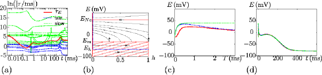
Figure 5: Non-Tikhonov asymptotics of the Courtemanche et al. 1998 model. (a) Characteristic times during a typical AP potential solution, as indicated by the legend. Red solid line: $\tau_{E}$, blue dashed line: $\tau$’s of superfast ($m$, $u_{a}$, $w$) and fast ($h$, $o_{a}$, $d$), green dash-dotted lines: $\tau$’s of other, slow variables. (b) Phase portrait of the fast subsystem (13). (c) Action potential upstroke, $\epsilon_{1}=\epsilon_{2}=1$ (solid red), $\epsilon_{1}=10^{-3}$, $\epsilon_{2}=1$ (dotted blue), $\epsilon_{1}=\epsilon_{2}=10^{-3}$ (dashed green), in the fast time $T=t/\epsilon_{2}$. (d) Same, for the whole AP in the slow time $t$. See also [Suckley-2004].

Next, we identify the fast variables with speeds comparable to the AP upstroke. This is also done by comparing the instantaneous values of the variables with the corresponding quasi-stationary values, and checking how their adiabatic elimination affects the AP, for the AP solution after the initial upstroke. In this way, we identify variables $h$, $o_{a}$ and $d$ as fast, with associated small parameter $\epsilon_{2}$.

Similar to N62, the transmembrane voltage is $\epsilon_{2}^{-1}$-fast only during the AP upstroke due to $\epsilon_{2}^{-1}$-large values of $I_{\mathrm{Na}}$ during that period, and is slow otherwise. This is due to nearly perfect switch behaviour of the gates $m$ and $h$. The definition of $I_{\mathrm{Na}}$ in this model is more complicated as there is also the $j$ gate; however $j$ is slow and does not change noticeably during the upstroke.

These considerations lead to the following parameterization of the model:

$$C_{M}{\mathrm{d}E}/{\mathrm{d}t} = -\left(\epsilon_{2}^{-1}I_{\mathrm{Na}}(E,m,h,j)+{\Sigma_{I}^{\prime}}(E,\dots)\right),$$

$$\epsilon_{1}\epsilon_{2}{\mathrm{d}m}/{\mathrm{d}t} = {(\hat{{\overline{m}}}(E;\epsilon_{2})-m)}/{\tau_{m}(E)},\qquad\hat{{\overline{m}}}(E;0)=M(E)\theta(E-E_{m}),$$

$$\epsilon_{2}{\mathrm{d}h}/{\mathrm{d}t} = {(\hat{{\overline{h}}}(E;\epsilon_{2})-h)}/{\tau_{h}(E)},\qquad\hat{{\overline{h}}}(E;0)=H(E)\theta(E_{h}-E),$$

$$\epsilon_{1}\epsilon_{2}{\mathrm{d}u_{a}}/{\mathrm{d}t} = {(\overline{u_{a}}(E)-u_{a})}/{\tau_{u_{a}}(E)},$$

$$\epsilon_{1}\epsilon_{2}{\mathrm{d}w}/{\mathrm{d}t} = {(\overline{w}(E)-w)}/{\tau_{w}(E)},$$

$$\epsilon_{2}{\mathrm{d}o_{a}}/{\mathrm{d}t} = {(\overline{o_{a}}(E)-o_{a})}/{\tau_{o_{a}}(E)},$$

$$\epsilon_{2}{\mathrm{d}d}/{\mathrm{d}t} = {(\overline{d}(E)-d)}/{\tau_{d}(E)},$$ (12)

$$\dots$$

where $I_{\mathrm{Na}}(E,m,h,j)=g_{Na}m^{3}hj(E-E_{Na})$ is the fast Na current and ${\Sigma_{I}^{\prime}}(E,\dots)$ represents all other currents. Here we have shown only equations that contain $\epsilon_{1}$ or $\epsilon_{2}$. All other equations are the same as in the original model.

As before, we adiabatically eliminate the superfast variables in the limit $\epsilon_{1}\rightarrow 0$, and turn $\epsilon_{2}\rightarrow 0$ in the fast time scale $T=t/\epsilon$. This gives the fast subsystem

$$C_{M}{\mathrm{d}E}/{\mathrm{d}T} = g_{Na}j(E_{Na}-E)M^{3}(E)\theta(E-E_{m})h,$$

$${\mathrm{d}h}/{\mathrm{d}T} = {(H(E)\theta(E_{h}-E)-h)}/{\tau_{h}(E)},$$

$${\mathrm{d}o_{a}}/{\mathrm{d}T} = {(\overline{o_{a}}(E)-o_{a})}/{\tau_{o_{a}}(E)},$$

$${\mathrm{d}d}/{\mathrm{d}T} = {(\overline{d}(E)-d)}/{\tau_{d}(E)}.$$ (13)

Notice that in (13) the equations for $o_{a}$ and $d$ depend on $E$, but equations for $E$ and $h$ do not depend neither on $o_{a}$ nor on $\mathrm{d}$. Thus, the evolution equations for $E$ and $h$ form a closed subsystem. This system is identical to (10), up to the values of parameters, definitions of the functions of $E$ and the presence of the slow variable $j$ as the factor at the maximal conductance of the Na current, $g_{Na}$. The phase portrait of (13), fig. 5(b), is similar to that of N62, fig. 4(b). So the peculiar features of the fast subsystem of N62 are not unique and are found in many cardiac models, including CRN.

With a view of a practical application of approximation (13), it is interesting to test its quantitative accuracy. This is illustrated in fig. 5, panel (c) for the shape of the upstroke in the fast time $T=t/\epsilon$, and panel (d) for the shape of the AP in the slow time $t$. We see that the approximation of the AP is very good in both limits $\epsilon_{1}\rightarrow 0$ and $\epsilon_{2}\rightarrow 0$, except for the upstroke: e.g. the peak voltage is overestimated by about 13 mV. This is mostly due to the limit $\epsilon_{1}\rightarrow 0$, i.e. replacement of $m$ with $\overline{m}(E)$. So the accuracy could be significantly and easily improved by retracting the limit $\epsilon_{1}\rightarrow 0$, which amounts to inclusion of the evolution equation for $m$ instead of the finite equation $m=\overline{m}(E)$. Most of the qualitative analysis remains valid. However, here for simplicity we stick to the less accurate but simpler case $\epsilon_{1}=0$. Notice that in fig. 5(b–d), we took $M(E)=1$, $H(E)=1$; the error introduced by that was small compared to other errors, particularly the error introduced by $m=\overline{m}(E)$.

4 Application to spatially distributed systems

Fronts.

We now use the fast Na subsystem of the cardiac excitation (13) to consider a propagation of an excitation front through a cardiac fibre. In one spatial dimension, this requres replacement of ordinary time derivatives with partial derivatives and adding a diffusion term into the equation for $E$:

$${\partial E}/{\partial t} = J(E)\theta(E-E_{m})h+D{\partial^{2}E}/{\partial x^{2}},$$

$${\partial h}/{\partial t} = {(\theta(E_{h}-E)-h)}/{\tau_{h}(E)},$$ (14)

where $J(E)=g_{Na}j(E_{Na}-E)M^{3}(E)$ and we have put $H(E)=1$. We consider solutions in the form of propagating fronts. For definiteness, let us assume the fronts propagating leftwards, so $E(x,t)=E(\xi)$, $h(x,t)=h(\xi)$, $\xi=x+ct$, $h(-\infty)=1$, $h(+\infty)=0$, $E(-\infty)=E_{-}$ and $E(+\infty)=E_{+}$. In this formulation, we have three constants characterizing the solutions, the prefront voltage $E_{-}$, the postfront voltage $E_{+}$ and the speed $c$. It is not obvious which combinations of the three parameters admit how many front solutions. So we have considered a “caricature” of (14) by replacing functions $J(E)$ and $\tau_{h}(E)$ in it with constants:

$${\partial E}/{\partial t} = J\theta(E-E_{m})h+D{\partial^{2}E}/{\partial x^{2}},$$

$${\partial h}/{\partial t} = {(\theta(E_{h}-E)-h)}/{\tau_{h}},$$ (15)

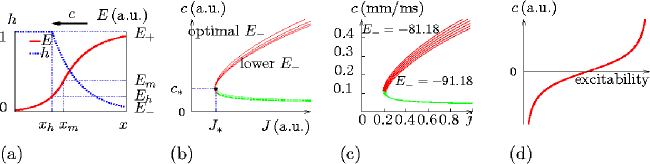
Figure 6: Fronts in the spatially distributed Na subsystem. (a) The structure of the front solution in the caricature model. (b) Speed of the fronts as function of excitability, at selected values of the pre-front voltage, in the caricature model (15). $J_{*}$ is minimal excitability at which propagation is possible at any $E_{-}$, and $c_{*}$ is the corresponding propagation speed. (c) Speed of the fronts as function of excitability, at selected values of pre-front voltage, in the Na subsystem of the CRN model (14). On (b) and (c), solid red lines, above and raising, are the stable branches and dashed green lines, below and decreasing, are the unstable branches. (d) For comparison: speed of the fronts in a typical Tikhonov front (fast susbsystem of the FHN model). See also [Biktashev-2002, Biktashev-Biktasheva-2005].

This system is piecewise linear and admits complete analytical investigation. Details can be found in [Biktashev-2002, Biktashev-2003]; here we only briefly outline the results. Fig. 6(a) illustrates a typical front solution. It exists if speed $c$ and pre-front voltage $E_{-}$ satisfy a finite equation involving also the constants $J$ and $\tau_{h}$. The resulting dependence of the conduction velocity $c$ on excitability $J$ for a few selected values of $E_{-}$ is shown in fig. 6(b). These front solutions exist only for $J$ at or above a certain minimum $J_{\min}$ which depends on $E_{-}$. For $J>J_{\min}(E_{-})$ there are two solutions with different speeds. Numerical simulations of PDE system (15) suggest that solutions with higher speeds are stable and solutions with lower speeds are unstable; this has been confirmed analytically by Hinch-2004.

The replacement of functions $J(E)$ and $\tau_{h}(E)$ with constants is a rather crude step. The purpose of the caricature is not to provide a good approximation, but to investigate qualitatively the structure of the solution set. To see if this structure is the same for the more realistic models, we have solved numerically the boundary-value problems for the front solutions in (14). There the role of the excitability parameter is played by the variable $j$. The results of the calculations are shown in fig. 6(c). Not only the topology of the solution set is the same, but the overall behaviour of $c(j,E_{-})$ in (14) is quite similar to that of $c(J,E_{-})$ in (15), despite the crudeness of the caricature.

PDE simulations show that approximation (14) overestimates the conduction velocity by almost 50% compared to the full model, and the error is again mainly due to the adiabatic elimination of the $m$ gate.

After eliminating the superfast variables $m$, $u_{a}$ and $w$ and the fast variables $h$, $o_{a}$ and $d$, and retaining the non-Tikhonov variable $E$, the slow subsystem of (12) has 16 equations. It describes the AP behind the front.

The most important conclusion is that for any particular value of the prefront voltage $E_{-}$ there is a certain minimum excitability $j_{\min}=j_{\min}(E_{-})$ and corresponding minimum propagation speed $c_{\min}=c_{\min}(E_{-})$, and for $j<j_{\min}$, no steady front solutions are possible. This is completely different from the behaviour in FitzHugh-Nagumo (FHN) type systems, where local kinetics are Tikhonov and a front is a trigger wave in a bistable reaction-diffusion system. A typical dependence of the speed of such a trigger wave on a slow variable is shown in fig. 6(d): it can be slowed down to a halt or even reversed. The reversed trigger waves describe backs of propagating pulses in FHN systems. Thus, questions about the shape of the backs of APs and propagating pulses, and the spectrum of propagation speeds of a propagating excitation wave in a tissue come to be closely related. In both questions, our new non-Tikhonov approach provides different answers from the traditional Tikhonov/FHN approach. We have already seen that the new description is more in line with the detailed ionic models regarding the back of an AP. In the next section, we demonstrate the advantage of the new approach regarding the fronts.

Dissipation of fronts.

The fast subsystem of a typical spatially-dependent cardiac excitation model, discussed in the previous section, only provides part of the answer. This description should be completed with the description of the slow movement. The fronts are passing so quickly through every given point that the values of the slow variables at that point change little while it happens. Away from the fronts, the fast variables keep close to their quasi-stationary values. In our asymptotics this means, in particular, that the fast Na channels are closed, and $E$ is not a fast but a slow variable. Assuming absence of spatially sharp inhomogeneities of tissue properties, simple estimates show that outside fronts, the diffusive current is much smaller than ionic currents, so dynamics of cells there are essentially the same as dynamics of isolated cells outside AP upstrokes.

Propagation of the next front depends on the transmembrane voltage $E$, which serves as parameter $E_{-}$, and the slow inactivation gate $j$ of the fast Na current. This dependence gives an equation of motion for the front coordinate $x(t)$,

$${\mathrm{d}x}/{\mathrm{d}t}=c(j(x,t),E(x,t)),$$ (16)

where the instantaneous speed of the front $c$ is determined by the values of $E$ and $j$ at the sites through which the front traverses (in case of $E$ this is the value which would be there if not the front). This can only continue as long as the function $c(j,E)$ remains defined, i.e while $j(x,t)>j_{\min}(E(x,t))$. If the front runs into a region where this is not satisfied, its propagation becomes unsustainable.

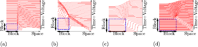
Figure 7: Effects of temporary propagation blocks. (a) In the CRN model. (b) In the FHN model. (c) In the caricature Na front. (d) In the Na subsystem of the CRN model. See also [Biktashev-Biktasheva-2005].

What will happen then is illustrated in fig. 7(a), where the parameter $g_{Na}$ was varied in space and time. To make the effect more prominent, we did not use smooth variation, but put $g_{Na}=0$ in the left half of the interval for some time and then restored it to its normal value. The propagating front reached this region while it was in the inexcitable state. The result was that the sharp front ceased to exist, it “dissipated”, and instead of an active front we observed a purely diffusive spread of the voltage. The excitability was restored a few milliseconds later, but the sharp front did not recover and diffusive spread of voltage continued, leading eventually to a complete decay of the wave. Note that the back of the propagating pulse was still very far when the impact that caused the front dissipation happened.

This is completely different from the behaviour of a FHN system in similar circumstances, shown in fig. 6(b). There propagation was blocked for almost the whole duration of the AP. And yet when the block was removed, the propagation of the excitation wave resumed. Only if the block stays so long that the waveback reaches the block site and the “wavelength” reduces to zero, the wave would not resume. Such considerations have lead to a widespread, would-be obvious assumption that shrinking of the excitation wave to “zero length” is a necessary condition and therefore a “cause” of the block of propagation of excitation waves [Weiss-etal-2000]. Comparison of panels (a) and (b) in fig. 6 shows that this is far from true for ionic cardiac models, where such reduction to zero length happens, but only as a very distant consequence, rather than a cause, of the propagation block. The true reason for the block is the disappearance of the fast Na current at the front, observed phenomenologically as its dissipation.

We expect that the condition $j>j_{\min}(E)$ can also serve as a condition of propagation in the non-stationary situation on the slow space time/scale. Moreover, we conjecture that the dissipation of the front will happen where and when the front runs into a region with $j<j_{\min}(E)$. This is illustrated by a simulation shown in fig. 6(c). It is a solution of the caricature system (15), where the excitability parameter $J$ has been maintained slightly above the threshold $J_{\min}(E_{-})$ outside the block domain, and slightly below it within the block domain. As a result, the front propagation has been stopped and never resumed even after the block has been removed. A similar simulation for the quantitatively more accurate fast subsystem of the CRN model, (14), is shown on panel (d). Both agree with what happens in the full model on panel (a), and both confirm that the condition $j<j_{\min}$ is relevant for causing front dissipation.

Break-ups and self-terminations of re-entrant waves

In two spatial dimensions, the condition $j<j_{\min}(E)$ may happen to a piece of a wavefront rather than the whole of it. Then instead of a complete block we observe a local block and breakup of the excitation wave. This happened in the episode shown in fig. 8.

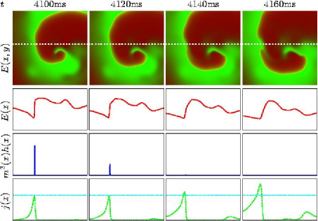
Figure 8: Analysis of a break-up of a re-entrant wave in a simulation similar to fig. 1. Top row: snapshots of the distribution of the transmembrane voltage, at the selected moments of time (designated above the panels). The other three rows: profiles of the key dynamic variables (designated on the left) along the dotted line shown on the top row panels, at the same moments of time. The scale of $E$ is $[-100\,\mathrm{mV},0\,\mathrm{mV}]$. The scale of $m^{3}h$ is $[0,0.15]$. The scale of $j$ is $[0,0.5]$. Cyan dash-dotted line on $j$ panels represents $j_{\min}$. See also [Biktashev-Biktasheva-2005].

The white dotted horizontal line on the top panels goes across the region where the propagating wave has been blocked and front has dissipated. The details of how it happened are analysed on the lower three rows, showing profiles of relevant variables along this dotted white line. The second row shows the profiles of $E$, which lose the sharp front gradient after $t=4100\,\mathrm{ms}$. The third row shows the peaks of the spatial distribution of the product $m^{3}h$; the sharpness of these peaks corresponds to the sharp localization of $I_{\mathrm{Na}}$ at the front, and their decay accompanies the process of the front dissipation. The most instructive is evolution of the profile of the $j$ variable shown on the bottom row. Consider the column $t=4100\,\mathrm{ms}$. The gradient of $j$ ahead of the front, i.e. to the left of the peak of $m^{3}h$, is positive, and the front is moving leftwards, i.e. towards smaller values of $j$. That is, the front moves into a less excitable area, left there after the previous rotation of the spiral wave. To the right of the peak of $I_{\mathrm{Na}}$ the gradient of $j$ is negative which corresponds to the fact that $j$ decreases during the plateau of the AP. Thus its maximal value at this particular time is observed at the front. This maximal value is, therefore, the value that should be considered in the condition of the dissipation, $j<j_{\min}(E)$.

As soon as the front has dissipated ($t\approx 4120\,\mathrm{ms}$), the profile of $j$ starts to raise, so the maximum of the $j$ profile observed at $t=4120\,\mathrm{ms}$ is the lowest one. From the fact that dissipation has started we conclude that this maximum is below the critical value $j_{\min}$. Assuming that dissipation usually happens soon after the condition $j<j_{\min}$ is satisfied (simulations of (14) show that this happens within a few milliseconds), this smallest maximum value should be close to $j_{\min}$, which gives an empirical method of determining $j_{\min}$ from numerical simulations of complete PDE models. For this particular episode the empirical value of $j_{\min}$ was found to be approximately 0.3. This is about 50% higher than the $j_{\min}$ predicted for the same range of voltages by (14); we attribute this to the approximation $m\approx\overline{m}$ which caused similar errors in the upstroke height and front propagation speeds.

5 Conclusion

Our new asymptotic approach for cardiac excitability equations has significant advantages over the traditional approaches. The fast subsystem, represented by equations (10) and (14), appears to be typical for cardiac models. This predicts that front propagation cannot happen at a speed slower than a certain minimum and at an excitability parameter lower than a certain minimum. When these conditions are violated the front dissipates and does not recover even after excitability is restored. We have obtained a condition for front dissipation in terms of an inequality involving prefront values of $j$ and $E$. This condition can be used for the analysis of break-up and self-termination of re-entrant waves in two and three spatial dimensions.

Acknowledgments

This work was supported in part by grants from EPSRC (GR/S43498/01, GR/S75314/01) and by an RDF grant from Liverpool University.

References

- [1] \harvarditem[Arnold et al.]Arnold, Afrajmovich, Il’yashenko & Shil’nikov1994Arnold-etal-1994 Arnold, V. I., Afrajmovich, V. S., Il’yashenko, Y. S. & Shil’nikov, L. P. (1994), Dynamical Systems V. Bifurcation Theory And Catastrophe Theory, Springer-Verlag.
- [2] \harvarditem[Biktashev]Biktashev2002Biktashev-2002 Biktashev, V. N. (2002), ‘Dissipation of the excitation wavefronts’, Phys. Rev. Lett. 89(16), 168102.
- [3] \harvarditem[Biktashev]Biktashev2003Biktashev-2003 Biktashev, V. N. (2003), ‘A simplified model of propagation and dissipation of excitation fronts’, Int. J. of Bifurcation and Chaos 13(12), 3605–3620.
- [4] \harvarditem[Biktashev & Biktasheva]Biktashev & Biktasheva2005Biktashev-Biktasheva-2005 Biktashev, V. N. & Biktasheva, I. V. (2005), ‘Dissipation of excitation fronts as a mechanism of conduction block in re-entrant waves’. To appear in Lect. Notes in Comput. Sci.
- [5] \harvarditem[Biktashev & Suckley]Biktashev & Suckley2004Biktashev-Suckley-2004 Biktashev, V. N. & Suckley, R. (2004), ‘Non-Tikhonov asymptotic properties of cardiac excitability’, Phys. Rev. Lett. 93(16), 168103.
- [6] \harvarditem[Biktasheva et al.]Biktasheva, Biktashev, Dawes, Holden, Saumarez & M.Savill2003Biktasheva-etal-2003 Biktasheva, I. V., Biktashev, V. N., Dawes, W. N., Holden, A. V., Saumarez, R. C. & M.Savill, A. (2003), ‘Dissipation of the excitation front as a mechanism of self-terminating arrhythmias’, IJBC 13(12), 3645–3656.
- [7] \harvarditem[Cherry & Fenton]Cherry & Fenton2004Cherry-Fenton-2004 Cherry, E. M. & Fenton, F. H. (2004), ‘Suppression of alternans and conduction blocks despite steep APD restitution: Electrotonic, memory, and conduction velocity restitution effects’, Am. J. Physiol. - Heart C 286, H2332–H2341.
- [8] \harvarditem[Courtemanche et al.]Courtemanche, Ramirez & Nattel1998Courtemanche-etal-1998 Courtemanche, M., Ramirez, R. J. & Nattel, S. (1998), ‘Ionic mechanisms underlying human atrial action potential properties: insights from a mathematical model’, Am. J. Physiol. 275, H301–H321.
- [9] \harvarditem[FitzHugh]FitzHugh1961FitzHugh-1961 FitzHugh, R. (1961), ‘Impulses and physiological states in theoretical models of nerve membrane’, Biophys. J. 1, 445–456.
- [10] \harvarditem[Hinch]Hinch2004Hinch-2004 Hinch, R. (2004), ‘Stability of cardiac waves’, Bull. Math. Biol. 66(6), 1887–1908.
- [11] \harvarditem[Hodgkin & Huxley]Hodgkin & Huxley1952Hodgkin-Huxley-1952 Hodgkin, A. L. & Huxley, A. F. (1952), ‘A quantitative description of membrane current and its application to conduction and excitation in nerve’, J. Physiol. 117, 500–544.
- [12] \harvarditem[Karma]Karma1994Karma-1994 Karma, A. (1994), ‘Electrical alternans and spiral wave breakup in cardiac tissue’, Chaos 4(3), 461–472.
- [13] \harvarditem[Karma et al.]Karma, Levine & Zou1994Karma-etal-1994 Karma, A., Levine, H. & Zou, X. Q. (1994), ‘Theory of pulse instabilities in electrophysiological models of excitable tissues’, Physica D 73, 113–127.
- [14] \harvarditem[Nagumo et al.]Nagumo, Arimoto & Yoshizawa1962Nagumo-etal-1962 Nagumo, J., Arimoto, S. & Yoshizawa, S. (1962), ‘An active pulse transmission line simulating nerve axon’, Proc. IRE 50, 2061–2070.
- [15] \harvarditem[Noble]Noble1962Noble-1962 Noble, D. (1962), ‘A modification of the Hodgkin-Huxley equations applicable to Purkinje fibre action and pace-maker potentials’, J. Physiol. 160, 317–352.
- [16] \harvarditem[Nolasco & Dahlen]Nolasco & Dahlen1968Nolasco-Dahlen-1968 Nolasco, J. B. & Dahlen, R. W. (1968), ‘A graphic method for the study of alternation in cardiac action potentials’, J. Appl. Physiol. 25, 191–196.
- [17] \harvarditem[Pontryagin]Pontryagin1957Pontryagin-1957 Pontryagin, L. S. (1957), ‘The asymptotic behaviour of systems of differential equations with a small parameter multiplying the highest derivatives’, Izv. Akad. Nauk SSSR, Ser. Mat. 21(5), 107–155.
- [18] \harvarditem[Suckley]Suckley2004Suckley-2004 Suckley, R. (2004), The Asymptotic Structure Of Excitable Systems Of Equations, PhD thesis, University of Liverpool, UK.
- [19] \harvarditem[Suckley & Biktashev]Suckley & Biktashev2003Suckley-Biktashev-2003 Suckley, R. & Biktashev, V. N. (2003), ‘Comparison of asymptotics of heart and nerve excitability’, Phys. Rev. E 68, 011902.
- [20] \harvarditem[Tikhonov]Tikhonov1952Tikhonov-1952 Tikhonov, A. N. (1952), ‘Systems of differential equations, containing small parameters at the derivatives’, Mat. Sbornik 31(3), 575–586.
- [21] \harvarditem[Tyson & Keener]Tyson & Keener1988Tyson-Keener-1988 Tyson, J. J. & Keener, J. P. (1988), ‘Singular perturbation theory of traveling waves in excitable media (a review)’, Physica D 32, 327–361.
- [22] \harvarditem[Weiss et al.]Weiss, Chen, Qu, Karagueuzian & Garfinkel2000Weiss-etal-2000 Weiss, J. N., Chen, P. S., Qu, Z., Karagueuzian, H. S. & Garfinkel, A. (2000), ‘Ventricular fibrillation: How do we stop the waves from breaking?’, Circ. Res. 87, 1103–1107.
- [23] \harvarditem[Wiener & Rosenblueth]Wiener & Rosenblueth1946Wiener-Rosenblueth-1946 Wiener, N. & Rosenblueth, A. (1946), ‘The mathematical formulation of the problem of conduction of impulses in a network of connected excitable elements, specifically in cardiac muscle’, Arch. Inst. Cardiologia de Mexico 16(3–4), 205–265.
- [24]