Semi-discrete composite solitons in arrays of quadratically nonlinear waveguides

Abstract

We demonstrate that an array of discrete waveguides on a slab substrate, both featuring the $\chi^{2}$ nonlinearity, supports stable solitons composed of discrete and continuous components. Two classes of fundamental composite solitons are identified: ones consisting of a discrete fundamental-frequency (FF) component in the waveguide array, coupled to a continuous second-harmonic (SH) component in the slab waveguide, and solitons with an inverted FF/SH structure. Twisted bound states of the fundamental solitons are found too. In contrast with usual systems, the intersite-centered fundamental solitons and bound states with the twisted continuous components are stable, in an almost entire domain of their existence.

Quadratically nonlinear ($\chi^{(2)}$) media, continuous or discrete, provide favorable conditions for the creation of optical solitons. The wave-vector mismatch and $\chi^{(2)}$ coefficient are efficient control parameters in this context, and the solitons display a variety of features due to their “multicolor” character. Accordingly, a great effort has been invested in the study of solitons in continuous hk93prl ; twh95prl (as reviewed in review1 ; review2 ) and (quasi-)discrete bcc97pre ; ppl98pre ; ktv04ol ; kvt04ol ; iss04prl ; mkf02pre ; cls03n $\chi^{(2)}$ media. In both cases, the solitons can find applications to all-optical switching ct99ol ; ppl03ol ; cls03n and light-beam steering.sbs98oqe ; vmk04pre

Waveguide arrays, i.e., one-dimensional (1D) discrete systems, exhibit properties that are absent in continuous media, such as anomalous or managed diffraction.cls03n Accordingly, discrete solitons are drastically different from their counterparts in continuous media, as was first predicted in the context of the $\chi^{(3)}$ nonlinearity cj88ol . Here we propose semi-discrete composite solitons in $\chi^{(2)}$ optical systems, that contain both discrete and continuous components, each carrying either the fundamental-frequency (FF) or second-harmonic (SH) wave. We demonstrate that stable semi-discrete solitons can be readily formed in a waveguide array coupled to a slab waveguide, both structures being made of a quadratically nonlinear material. We study two most interesting species of semi-discrete solitons. Type-A ones consist of a discrete FF component in the waveguide array, coupled to a continuous SH component in the slab waveguide. Conversely, type-B solitons feature continuous FF and discrete SH components in the slab and discrete array, respectively.

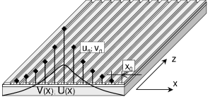
Figure 1: Schematic of the proposed setting.

The proposed setting is displayed in Fig. 1. It includes the periodic array of waveguides, with a spacing $x_{0}$, mounted on top of (or buried into) the slab waveguide. Both the array and slab are made of a $\chi^{(2)}$ material, such as $\mathrm{LiNbO_{3}}$ or $\mathrm{KTiOPO_{4}}$. A rigorous coupled-mode theory for such composite waveguides can be developed by a straightforward generalization of that available for a single discrete waveguide coupled to the slab vh96oc . Thus, we arrive at a system including a set of ordinary differential equations for the discrete array, coupled to a partial differential equation for the slab. In case A, the coupled equations take the following normalized form:

$$i\frac{\displaystyle d\phi_{n}}{\displaystyle d\zeta}+\varrho\left(\phi_{n-1}+\phi_{n+1}\right)+\phi_{n}^{\ast}\Psi(\zeta,n)=0,$$ (1a)

$$i\frac{\displaystyle\partial\Psi}{\displaystyle\partial\zeta}+\frac{\displaystyle 1}{\displaystyle 2}\frac{\displaystyle\partial^{2}\Psi}{\displaystyle\partial\eta^{2}}+\beta\Psi+\frac{\displaystyle 1}{\displaystyle 2}\sum_{n}\phi_{n}^{2}\delta(\eta-n)=0,$$ (1b)

and in case B they are written as

$$i\frac{\displaystyle\partial\Phi}{\displaystyle\partial\zeta}+\frac{\displaystyle 1}{\displaystyle 2}\frac{\displaystyle\partial^{2}\Phi}{\displaystyle\partial\eta^{2}}+\Phi^{\ast}\sum_{n}\psi_{n}\delta(\eta-n)=0,$$ (2a)

$$i\frac{\displaystyle d\psi_{n}}{\displaystyle d\zeta}+\beta\psi_{n}+\varrho\left(\psi_{n-1}+\psi_{n+1}\right)+\frac{\displaystyle 1}{\displaystyle 2}\Phi^{2}(\zeta,n)=0.$$ (2b)

Here, the normalized coordinates are $$\zeta=z/z_{0} \eta=x/x_{0} z x z_{0}=Kx_{0}^{2} K \beta \delta(\eta) \varrho=c_{d}z_{0} c_{d} \phi_{n} \Phi \psi_{n} \Psi u_{n},U v_{n},V \phi_{n}=(z_{0}/\sqrt{x_{0}})\sqrt{2\gamma_{d}\gamma_{c}}u_{n} \Psi=z_{0}\gamma_{d}V \psi_{n}=(z_{0}/x_{0})\gamma_{c}v_{n} \Phi=(z_{0}/\sqrt{x_{0}})\sqrt{2\gamma_{d}\gamma_{c}}u_{n}U \gamma_{d,c}=\frac{\epsilon_{0}\omega}{4P_{d,c}\sqrt{P_{c,d}}}{\int_{A_{d,c}}}dA\mathbf{\hat{e}}_{n,c}^{\ast}(\omega)\cdot\mathbf{\hat{\chi}}(2\omega,\omega)\mathbf{\hat{e}}_{n,c}^{\ast}(\omega)\mathbf{\hat{e}}_{c,n}(2\omega) \gamma_{c,d}=\frac{\epsilon_{0}\omega}{2P_{d,c}\sqrt{P_{c,d}}}{\int_{A_{c,d}}}dA\mathbf{\hat{e}}_{c,n}^{\ast}(2\omega)\cdot\mathbf{\hat{\chi}}(\omega,\omega)\mathbf{\hat{e}}_{n,c}(\omega)\mathbf{\hat{e}}_{n,c}(\omega) P_{d} P_{c} A_{d} A_{c} \mathbf{\hat{e}}_{n}(x,y) \mathbf{\hat{e}}_{c}(x) \varrho=1$$ and , where and are, respectively, the distances in the propagation and transverse directions, , is the propagation constant of the corresponding continuous mode, is the effective wave vector mismatch, is the delta-function, and is the normalized coupling constant between adjacent waveguides in the array, where is the coupling constant in physical units, as predicted by the coupled-mode theory.vh96oc The normalized field amplitudes at the FF, and , and at the SH, and , are proportional to their counterparts, and , measured in physical units: , and , , where , in cases A and B, respectively, with and the power in the stripe waveguide and the power density in the slab waveguide, and the transverse areas of the stripe waveguide and slab waveguide between two adjacent stripes, respectively, and and fundamental modes of the stripe and slab waveguides. In this paper, we focus on the case of , which adequately represents the generic situation.

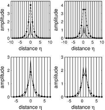
Figure 2: Field profiles of composite solitons. Here and in the next figure, top and bottom panels correspond to the solitons of types A and B, respectively, whereas left and right panels display odd and even solitons. Vertical lines designate the location of discrete waveguides. The wave vector mismatch is $\beta=0$, and the soliton wavenumber is $\lambda=3$ and $\lambda=1.5$, in cases A and B, respectively.

The above equations were derived for the case when the FF and SH fields have the same (TE or TM) polarization. Using the general coupled-mode description vh93jlt , the system can be extended for the case of two polarizations, which will lead to a type-II $\chi^{(2)}$ interactionreview1 ; review2 involving two different FF components. This case will be presented elsewhere.

Both variants of the model (A and B) neglect direct FF-SH interactions in the same waveguide, as they are suppressed by the large natural mismatch, while we assume that care is taken to minimize the mode mismatch, between the continuous and discrete waveguides. Such requirements can be easily fulfilled, as the geometry gives rise to different propagation constants for the same frequency in the waveguides of the two types. A model which takes into regard the residual SH-FF coupling in each waveguide can be easily considered too, but cases A and B, as defined above, are the most interesting ones. Note also that in this geometry the overlap between the FF and SH is smaller, as compared to the case in which FF-SH interactions in the same waveguide are employed.

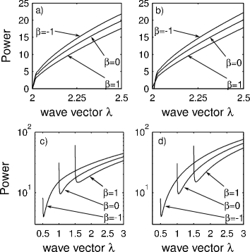
Figure 3: The total power $P$ of the semi-discrete solitons vs. the wavenumber $\lambda$.

Composite solitons amount to stationary solutions of systems (1) and (2) in the form of $\phi_{n}(\zeta)=\bar{\phi}_{n}\exp(i\lambda\zeta)$, $\Psi(\eta,\zeta)=\bar{\Psi}(\eta)\exp(2i\lambda\zeta)$ and $\psi_{n}(\zeta)=\bar{\psi}_{n}\exp(2i\lambda\zeta)$, $\Phi(\eta,\zeta)=\bar{\Phi}(\eta)\exp(i\lambda\zeta)$, respectively, where $\lambda$ is the soliton’s wavenumber. Inserting these expressions in the underlying equations, we solved the resulting systems by dint of the Newton-Raphson method. Similar to the ordinary discrete solitons, the composite ones can be odd or even: the former ones are centered at a site of a discrete waveguide, whereas even solitons are intersite-centered. Typical examples of odd and even composite solitons are displayed for both cases, A and B, in Fig. 2.

To examine the stability of the composite solitons, we have first applied the Vakhitov-Kolokolov (VK) criterion vk73rqe , which predicts that the necessary stability condition is $dP/d\lambda>0$, where $P$ is the total power [which is the single dynamical invariant of Eqs. (1) and (2)], $P(\lambda)=2\int_{-\infty}^{+\infty}|\left\{\Psi,\Phi\right\}|^{2}d\eta+\sum_{n}|\left\{\phi_{n},\psi_{n}\right\}|^{2}$, in cases A and B, respectively. The result is displayed in Fig. 3, which shows that (as may be expected) the solitons exist above the band of linear waves of the discrete subsystem, i.e., for $\lambda>2$ in case A, and $\lambda>1+\beta/2$ in case B, and both odd and even solitons are VK-stable in most of their existence domain. The prediction is significant, as even solitons are always unstable in ordinary discrete systems. Note that the power of odd solitons is slightly smaller than that of even ones.

A noteworthy feature is that A-type solitons exist up to $P=0$, while their B-type counterparts have a cutoff in terms of $P$. This can be explained by noting that the limit of $P\rightarrow 0$ corresponds to the limit of broad (quasi-continuous) small-amplitude solitons. Straightforward analysis of Eqs. (1a) demonstrates that this limit exists indeed, reducing to $i\tilde{\phi}_{\zeta}+\tilde{\phi}_{\eta\eta}+|\tilde{\phi}|^{2}\tilde{\phi}/\left(2\left(4-\beta\right)\right)=0$, $\tilde{\Psi}=\tilde{\phi}^{2}/\left(2(4-\beta)\right)$, with $\{\tilde{\phi},\tilde{\Psi}\}=\{\phi_{n}e^{-2i\zeta},\Psi e^{-4i\zeta}\}$. On the other hand, the same limit, if applied to Eqs. (2a), amounts to a linear asymptotic equation, $i\Phi_{\zeta}+\Phi_{\eta\eta}=0$, which gives rise to no soliton solutions.

Full stability of the solitons was examined in direct simulations of Eqs. (1) and (2), which completely corroborate the predictions of the VK criterion. In particular, those composite solitons of the B-type which are VK-unstable as per Fig. 3 decay into linear waves.

We have also studied the twisted solitons, built as out-of-phase bound states of two odd ones, see examples of A- and B-type solitons with a twisted FF component in Fig. 4. Their stability was also examined by means of both the VK criterion (see Fig. 4) and in direct simulations. The results demonstrate that the semi-discrete twisted solitons exist if their wavenumber $\lambda$ exceeds a cut-off value, which depends on the mismatch $\beta$, and they are stable in almost the entire existence domain. By contrast, in continuous $\chi^{(2)}$ media twisted solitons are always unstable review1 ; review2 . In a small region near the cut-off the twisted composite solitons are unstable too. The cut-off being well separated from the band of linear waves, in simulations the unstable twisted solitons do no decay into linear waves, but rather evolve into a fundamental odd soliton or split in two such solitons.

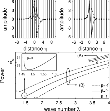
Figure 4: Top panels: field profiles of twisted composite solitons of types A (left) and B (right). In both cases, the wave vector mismatch and soliton’s wavenumber are $\beta=0$ and $\lambda=3.6$. The bottom panel shows the total power $P$ vs. $\lambda$, the inset blowing up a vicinity of the cutoff point (stability border) on the curve for $\beta=0$.

To summarize, we have shown that stable composite solitons, fundamental and twisted ones, can be supported by a slab waveguide coupled to an array of waveguides, both made of a $\chi^{(2)}$ material. This new species of semi-discrete solitons features unusual properties, viz., stability of intersite-centered fundamental solitons, and of states with the twisted continuous component. One can envisage that this system may also support walkingtmm96prl semi-discrete solitons, and that similar solitons can be found in dual discrete-continuous systems with the Kerr nonlinearity, as well as in multidimensional $\chi^{(2)}$ systems.

This work has been supported by the NSF Grant No. ECS-0523386 and DoD STTR Grant No. FA9550-04-C-0022.

References

- (1) K. Hayata and M. Koshiba, Phys. Rev. Lett. 71, 3275 (1993).
- (2) W. E. Torruellas, Z. Wang, D. J. Hagan, E. W. VanStryland, G. I. Stegeman, L. Torner, and C. R. Menyuk Phys. Rev. Lett. 74, 5036 (1995).
- (3) C. Etrich, F. Lederer, B.A. Malomed, T. Peschel, and U. Peschel, Progr. Opt. 41, 483 (2000).
- (4) A. V. Buryak, P. Di Trapani, D. V. Skryabin, and S. Trillo, Phys. Rep. 370, 63 (2002).
- (5) O. Bang, P. L. Christiansen, and C. B. Clausen, Phys. Rev. E56, 7257 (1997).
- (6) T. Peschel, U. Peschel, and F. Lederer, Phys. Rev. E57, 1127 (1998).
- (7) B. A. Malomed, P. G. Kevrekidis, D. J. Frantzeskakis, H. E. Nistazakis, and A. N. Yannacopoulos, Phys. Rev. E65, 056606 (2002).
- (8) Y. V. Kartashov, L. Torner, and V. A. Vysloukh, Opt. Lett. 29, 1117 (2004).
- (9) Y. V. Kartashov, V. A. Vysloukh, and L. Torner Opt. Lett. 29, 1399 (2004).
- (10) R. Iwanow, R. Schiek, G. I. Stegeman, T. Pertsch, F. Lederer, Y. Min, and W. Sohler, Phys. Rev. Lett. 93, 113902 (2004).
- (11) D. N. Christodoulides, F. Lederer, and Y. Silberberg, Nature 424, 817 (2003).
- (12) C. B. Clausen and L. Torner, Opt. Lett. 24, 7 (1999).
- (13) T. Peschel, U. Peschel, and F. Lederer, Opt. Lett. 28, 102 (2003).
- (14) R. Schiek, Y. Baek, G. I. Stegeman, and W. Sohler, Opt. Quantum Electron. 30, 861 (1998).
- (15) R. A. Vicencio, M. I. Molina, and Yu. S. Kivshar, Phys. Rev. E70, 026602 (2004).
- (16) D. Christodoulides and R. Joseph, Opt. Lett. 13, 794 (1988).
- (17) R. Vallée and G. He, Opt. Commun. 126, 293 (1996).
- (18) R. Vallée and G. He, J. Lightwave Tech. 11, 1196 (1993).
- (19) M. G. Vakhitov and A. A. Kolokolov, Radiophys. Quantum Electron. 16, 783 (1973).
- (20) L. Torner, D. Mazilu, and D. Mihalache, Phys. Rev. Lett. 77, 2455 (1996).