Drift of Particles in Self-Similar Systems and its Liouvillian Interpretation

Abstract

We study the dynamics of classical particles in different classes of spatially extended self-similar systems, consisting of (i) a self-similar Lorentz billiard channel, (ii) a self-similar graph, and (iii) a master equation. In all three systems the particles typically drift at constant velocity and spread ballistically. These transport properties are analyzed in terms of the spectral properties of the operator evolving the probability densities. For systems (i) and (ii), we explain the drift from the properties of the Pollicott-Ruelle resonance spectrum and corresponding eigenvectors

I Introduction

Billiard systems have long served as paradigm models to study the foundations of statistical mechanics in connection to ergodic theoryArnold-Avez ; Sinai70 . In the recent years the study of transport properties of ensembles of particles in spatially extended systems, like diffusion in the Lorentz gas or multi-baker map Gasp ; tasaki and heat conduction in similar systems alonso1 ; alonso2 ; Leyvraz , has proven to be very fruitful in establishing connections between irreversible phenomena at the macroscopic scales and the chaotic properties of the reversible classical dynamics at the microscopic scales GaspB ; Dorfman .

In this respect an essential tool is the Liouvillian formulation of the dynamics. In this formulation, instead of considering the behavior of individual trajectories, we consider the evolution of a density $\rho_{0}(X)$ of initial conditions. This density evolves in phase space according to the Liouville equation $\partial_{t}\rho_{t}(X)+\hat{L}\rho_{t}(X)=0$, where $\rho_{t}(X)$ represents the density at time $t$ in phase space of points $X$ and the operator $\hat{L}=\{H,\cdot\}$ with $H$ the Hamiltonian of the system and $\{\cdot,\cdot\}$ the Poisson bracket is called the Liouvillian operator. This equation is integrated using the initial condition $\rho_{0}(X)$ Goldstein . We write its solution in the form $\rho_{t}(X)=(\hat{P}^{t}\rho_{0})(X)$ where we introduced the evolution operator $\hat{P}^{t}$ known as the Perron-Frobenius operator. When we are interested in the future time evolution of the system we may analyze this operator in terms of the Pollicott-Ruelle resonance spectrum $\{s_{j}\}$ of the chaotic systems Ruelle , which determines the decay rates of the system. That is, for long times, the density can be decomposed on modes which decay exponentially in time $\rho(X,t)\sim\sum_{j}e^{s_{j}t}c_{j}\psi_{j}(X)$ with the $c_{j}$ determined by the initial condition. Within this theoretical framework, macroscopic properties have been related to microscopic quantities. In particular it has been applied to billiard systems which are spatially periodic and whose extension is infinite in one or two directions GaspB . For these systems, analytical results can be obtained using the Bloch theorem. In fact, expanding the functions like densities $\rho$ and eigenstates of the Liouville operator $\psi_{j}$ in Fourier series it is possible to analyze the problem in the finite domain of a unit cell instead of the infinite domain of the extended billiard, and compute quantities like eigenvalues as function of the wavenumber.

In studying the application of this formalism to situations of physical interest, an important problem concerns the characterization of classes of systems other than spatially periodic ones, where one can successfully apply the spectral theory of the evolution operator.

Here we study a class of extended billiard models with a self-similar structure and show how the techniques described above can be transposed to such systems. By self-similar billiard, we mean a billiard made up of a collection of cells with a one-dimensional lattice structure, where the cell sizes increase exponentially with their indices. Because of this property, particles will move in a preferred direction and therefore have a mean drift. That is, contrary to the periodic case, a density of particles drifts with constant velocity and does not diffuse. It is our goal to provide a theoretical understanding of these properties, based upon the spectral analysis of the evolution (Perron-Frobenius) operator of the system.

By understanding we mean that, although we do not obtain explicit solutions for the eigenvalues and eigenvectors of the evolution operator, we show that they verify two properties which are essential to produce this drift. Thus, we establish the connection between a transport property of macroscopic nature and the evolution operator acting on phase-space trajectories, for a new class of spatially extended systems.

A comparison between different levels of description is achieved by considering successively a fully deterministic self-similar billiard, then introducing a mesoscopic model with stochastic collision rules, and finally a marcoscopic model in the form of a master equation.

The article is organized as follows. Section II describes the self-similar billiard and the evolution of a particle in it. We identify two properties which characterize the spectrum of the evolution operator and discuss their consequences on the evolution of statistical ensembles. In order to help understand these features, we introduce, in Sec. III, a class of self-similar graphs. We show this system verifies two properties similar to those of the billiard. In Sec. IV, a phenomenological approach is given, based on a Master equation, for which we obtain exact expressions for the drift velocity and the mean square displacement. This provides theoretical predictions for the billiard and the graph models which are compared to numerical computations. Conclusions are drawn in Sec. V.

II Self-similar billiards

We will consider self-similar billiard chains such as shown in Fig. 2, which consist of an infinite collection of two-dimensional cells, shown in Fig. 1, glued together along a horizontal axis. Each cell contains convex scatterers and is open so as to allow particles to flow from one cell to the next. The shapes of the cells are identical, but their sizes are taken to grow exponentially with their indices. The overall geometry is such that upon combined shifting and rescaling the whole billiard is unchanged.

II.1 Definition of the Model

We consider a self-similar billiard chain based on the Lorentz channel GaspB . The reference cell is represented in Fig. 1. It is a region defined by the exterior of five disks, four of which are half disks, located at the corners of the cell and shared with the neighboring cells, and one located at the center of the cell. The dissymmetry between the left- and the right-hand sides depends on the scaling parameter $\mu$ ($\mu=1$ is the symmetric case). Given the value of $\mu$, there are three other parameters, namely $D$, $R$ and $r$, which, as shown in Fig. 1, determine respectively the horizontal width of the reference cell, the radii of the external disks and the radius of the center disk. Of these three pamarameters, only the ratios $R/D$ and $r/D$ are actually relevant. Notice the mirror symmetry of the unit cell about its center under the transformation $\mu\to 1/\mu$. Appendix A details the restrictions imposed on the values of the parameters, chosen so that the self-similar billiard shares the hyperbolicity of the Lorentz channel.

The two vertical segments of lengths $\Delta/\sqrt{\mu}$ and $\Delta\sqrt{\mu}$, with $\Delta\equiv\sqrt{3}D-2R$, at the left and right boundaries will be referred to as the windows of the cell, because a particle that goes across them moves from one cell to one of its neighbors, as will be detailed below.

Figure 1: Left Panel : The reference cell geometry. A detailed description is presented in appendix A. Here it is sufficient to note that $\Delta=\sqrt{3}D-2R$ and that with this choice the usual Lorentz channel is retrieved for $\mu=1$. Right Panel : The arrows on the right pannel represent schematically the matching condition : A trajectory leaving a cell from the right is reinjected to the left with a change of vertical coordinate $y=h\to y=\frac{h}{\mu}$ and the velocity changed according to $v\to\frac{v}{\mu}$.

It will be convenient to take $D=1$ and rescale $R$ and $r$ accordingly. Thus our billiard is characterized by $\mu$, $R/D$ and $r/D$.

The whole chain is constructed by adding a cell to the right of the reference cell, identical in shape but with all its lengths multiplied by $\mu$ and another one to the left with all the lengths divided by $\mu$. We repeat this construction in such a way that in the $i$th cell to the right all the lengths are multiplied by $\mu^{i}$ and, equivalently, by $\mu^{-i}$ to the left. The resulting billiard chain depicted in Fig. 2, is so constructed that the mirror symmetry with respect to the transformation $\mu\to 1/\mu$ remains.

Figure 2: The self-similar billiard and a trajectory for $\mu>1$, $1/\mu<1$ and $\mu=1$ respectively. Notice the symmetry of the billiard under $\mu\to 1/\mu$ and $x\to-x$.

Now we consider a particle moving inside the billiard with velocity $\vec{v}$. Figure 2 shows such a trajectory. As the particle moves from one cell to a neighboring one, the length scales change by a factor $\mu$, so that the characteristic time between collisions with the walls changes accordingly (the speed stays constant). Equivalently we can rescale the velocity by $\mu$ and keep the length scales unchanged. That is, in going from one billiard cell to the next, say from left to right, the following transformations are equivalent :

$$\left\{\begin{array}[]{c}\vec{v}\to\vec{v}\\ l\to\mu l\end{array}\right\}\Leftrightarrow\left\{\begin{array}[]{c}\vec{v}\to\frac{\vec{v}}{\mu}\\ l\to l\end{array}\right\}.$$ (1)

In both transformations the time between collisions with the walls is shorter ($\mu<1$) or longer ($\mu>1$) by a factor $\mu$.

Therefore we can analyze the dynamics on the self-similar billiard in terms of the dynamics in a periodic billiard if, instead of rescaling the size of the cell, we rescale the velocity. This way, the dynamics on the infinite self-similar billiard chain can be reduced to the dynamics on a single cell, provided the matching conditions given in Table 1 are imposed.

			Exit to the right	Exit to the left
position	$\vec{r}$	:	$(D,h)\quad\to\quad(0,h/\mu)$	$(0,h^{\prime})\quad\to\quad(D,h^{\prime}\mu)$
velocity	$\vec{v}$	:	$(v_{x},v_{y})\quad\to\quad(v_{x}/\mu,v_{y}/\mu)$	$(v_{x},v_{y})\quad\to\quad(v_{x}\mu,v_{y}\mu)$

Table 1: Matching conditions for trajectories crossing from one side of the cell to the other, as depicted on the right pannel of Fig. 1. The notations $h$ and $h^{\prime}$ are detailed in the text.

In Table 1, $h$ is the $y$ coordinate of the trajectory escaping through the right window, $-\sqrt{\mu}\Delta/2<h<\sqrt{\mu}\Delta/2$ and $h^{\prime}$, that of the trajectory escaping through the left window, $-\Delta/(2\sqrt{\mu})<h^{\prime}<\Delta/(2\sqrt{\mu})$. For the collisions with the walls the dynamics is determined by the Birkhoff map GaspB $(s,v_{\mathrm{t}})_{n}\to(s,v_{\mathrm{t}})_{n+1}$ of our modified Lorentz channel. Here the variable $s$ represents the arc-length along the unit cell boundary and $v_{\mathrm{t}}$ the projection of the normalized velocity ($|v|=1$) to the vector tangent to the boundary. This map, together with Table 1, provides the map for the evolution of a particle in the self-similar billiard, using only one cell. The matching conditions given in table 1 are analogous to periodic boundary conditions for a periodic billiard without the self-similar structure of our billiard.

The construction of the self-similar billiard we have presented is general and can be used to construct other self-similar billiards by changing the choice of the unit cell. The crucial point is that the cells are scaled uniformly by the factor $\mu$ at every step of the hierarchy.

To our knowledge, we are the first to consider a billiard with such a geometry.

II.2 Poincaré Map

As we have shown, the evolution on a self-similar billiard can be considered on a single cell, provided we change the speed of the particle at every time it crosses the windows. The mapping from one point of the boundary to the next can be described by the variables $s$ and $v_{\mathrm{t}}$. Let $\xi$ denote this pair of variables. The map,

$$\xi_{n+1}=\phi(\xi_{n}),$$ (2)

which determines the sequence of points visited on the boundary and the corresponding projection of the normalized velocity to the tangent vector, is called the ”Poincaré map”. The area where $\xi$ lives defines the Poincare surface of section $\mathcal{P}$.

This Poincaré map misses the information on the speed, which we can restore as follows. To consider the change of speed we need to keep track of the cell where the particle is located after the $n$ iterations. Let us introduce a new variable $I_{n}$, which takes integer values and labels the cell where the particle is at the $n$th iteration of the map. We defined the jump function $a(\xi)$, such that

$$I_{n+1}=I_{n}+a(\xi_{n}),$$ (3)

where $a(\xi_{n})=1$ if $\phi(\xi_{n})$ has the spatial coordinate $s_{n+1}$ on the right window, and $a(\xi_{n})=-1$ if $\phi(\xi_{n})$ has the spatial coordinate $s_{n+1}$ on the left window. Otherwise $a(\xi_{n})=0$.

Using the variable $I$ we can determine the actual speed from Eq. (1). Equivalently, we can say that the time it takes a trajectory at a (phase space) point $\xi$ on the boundary to intersect again with the boundary of the billiard depends on $I$ as

$$T(\xi,I)=\frac{L(\xi)}{v}\mu^{I}$$ (4)

where $L(\xi)$ is the length of the trajectory between intersections at $\xi$ and $\phi(\xi)$ of the trajectory with the boundary of the unit cell and $v$ is the speed of the particle.

Now we have a complete description of the dynamics in the self-similar billiard. Every point of phase space is characterized by $X=[\xi,\tau,I]$ with $0<\tau<T(\xi,I)$ a new variable that restores the position between collisions. The complete flow $\Phi^{t}(X)$ can be specified using these coordinates. This decomposition of the flow in terms of a Poincaré map and the variable $\tau$ along the trajectory issued from the Poincaré section is called a suspension flow. It can be implemented in billiards and other type of systems Sinai .

II.3 Evolution of Statistical Ensembles

Consider now an arbitrary distribution of initial conditions. The evolution of this statistical ensemble is determined by the Perron-Frobenius operator

$$(\widehat{P}^{t}\rho)(X)=\rho(\Phi^{-t}X)\ ,$$ (5)

which requires knowledge of the backward dynamics given by

$$\Phi^{-t}(\xi,\tau,I)=\left\{\begin{array}[]{l}(\xi,\tau-t,I),\qquad{\rm if}\quad 0\leq t<\tau,\\ (\phi^{-1}\xi,\tau-t+T(\phi^{-1}\xi,I-a(\phi^{-1}\xi)),I-a(\phi^{-1}\xi)),\\ \qquad{\rm if}\quad\tau\leq t<\tau+T(\phi^{-1}\xi,I-a(\phi^{-1}\xi)),\\ \vdots\end{array}\right.$$ (6)

At $t=\tau$ we cross the section $\mathcal{P}$ and we have to identify $[\xi,0,I]=[\phi^{-1}\xi,T(\phi^{-1}\xi,I-a(\phi^{-1}\xi)),I-a(\phi^{-1}\xi)]$. The interpretation is the following : for a particle in the cell $I$, its position and velocity are completely specified by $\xi$, which provides both the direction of the velocity and the last point of intersection with the perimeter of the cell. Moving a distance $\tau$ along the line going from this point of intersection in the direction of the velocity (both specified by $\xi$) we retrieve the exact position of the particle.

Now running the time backwards at $t=\tau$ we are just at the point of intersection with the billiard. This point is also the end of the segment issued from $\phi^{-1}(\xi)$, the previous intersection with the perimeter and at $\tau=T(\phi^{-1}\xi,I-a(\phi^{-1}\xi))$ which is the upper limit for the possible values of $\tau$ that start at $\phi^{-1}(\xi)$, with the corresponding direction. This intersection is not necessarily in the same cell $I$. The dependence on $I-a(\phi^{-1}\xi)$ indicate that the point $\phi^{-1}(\xi)$ is in the cell $I-a(\phi^{-1}\xi)$. This identification is made at every point of intersection.

In general, we can write Eq. (6) under the compact form,

$$\Phi^{-t}[\xi,\tau,I] = \left[\phi^{-n}\xi,\tau-t+\sum_{i=1}^{n}T\left(\phi^{-i}\xi,I-\sum_{j=1}^{i}a(\phi^{-j}\xi)\right),I-\sum_{i=1}^{n}a(\phi^{-i}\xi)\right],$$

$$\mathrm{if}\quad 0<\tau-t+\sum_{i=1}^{n}T\left(\phi^{-i}\xi,I-\sum_{j=1}^{i}a(\phi^{-j}\xi)\right)<T\left(\phi^{-n}\xi,I-\sum_{j=1}^{n}a(\phi^{-j}\xi)\right)$$

This construction introduces a small generalization of the treatment of periodic billiards described in Gas96 . More details can be found in that article.

This suspension flow formalism of the billiard dynamics has two main advantages : (i) it provides a method to simulate the dynamics of particles in extended billiards and, (ii) it can be used (at least formally) to determine the spectrum of the evolution operator as shown in Pollicott ; Gas96 . The generalization is direct, the only difference being the dependence of $T$ on $I$, the cell index.

Next we present the results relevant to this generalization and deduce two properties of the spectrum of the Perron-Frobenius operator that follow from the self-similar structure.

II.4 Two Properties of the Spectrum of the self-similar Billiard

Following Gas96 , by a Laplace transform of the Perron-Frobenius operator Eq. (5) and using Eq. (II.3), we obtain the following equation for the Pollicott-Ruelle resonance spectrum $\{s\}$ and the associated eigenstates $\{b_{s}\}$,

$$R_{s}b_{s}[\xi,I]=b_{s}[\xi,I],$$ (8)

with $R_{s}$ defined by

$$R_{s}f_{s}[\xi,I]=\exp[-sT(\phi^{-1}\xi,I-a(\phi^{-1}\xi))]f_{s}(\phi^{-1}\xi,I-a(\phi^{-1}\xi)).$$ (9)

In this expression, the operations must be understood in the following order : First take $\xi\to\phi^{-1}\xi$ everywhere and then $I\to I-a(\phi^{-1}\xi)$. The operator $R_{s}$ can be considered as a reduced Perron-Frobenius operator which evolves densities between successive crossings of the surface of section. A formal eigenstate can be obtained by successive applications of this operator to the identity. That is,

$$b_{s}[\xi,I] \equiv \lim_{n\to\infty}R_{s}^{n},$$ (10)

$$= \prod_{j=1}^{\infty}\exp\left[-sT\left(\phi^{-j}\xi,I-\sum_{i=1}^{j}a(\phi^{-i}\xi)\right)\right],$$

$$= \prod_{j=1}^{\infty}\exp\left[-\frac{s}{v}L(\phi^{-j}\xi)\mu^{I-\sum_{i=1}^{j}a(\phi^{-i}\xi)}\right],$$

which satisfies

$$R_{s}b_{s}=b_{s}.$$ (11)

Here we used Eq. (4) to obtain the last equality in Eq. (10). Similarly, an eigenstate $\tilde{b}_{s}$ of the adjoint operator can be obtained.

Now, we assume that a value of $s$, i. e. a Pollicott-Ruelle resonance, is known and thus the formal expression of $b_{s}$, Eq. (10), defines the corresponding eigenstate. We want to show that, given the pair $s$ and $b_{s}[\xi,I]$ (normalized) that satisfies

$$(R_{s}b_{s})[\xi,I]=b_{s}[\xi,I],$$ (12)

there corresponds a pair $s\mu$, $b_{s\mu}$ such that

$$(R_{s\mu}b_{s\mu})[\xi,I]=b_{s\mu}[\xi,I],$$ (13)

i. e. $s\mu$ is also a resonance.

In order to show this, we make the following ansatz : $b_{s\mu}[\xi,I]=b_{s}[\xi,I+1]$. First notice $b_{s\mu}$ exists and it is normalized by construction. We need to check that Eq. (13) is satisfied :

$$(R_{s\mu}b_{s\mu})[\xi,I] = \exp[-s\mu T(\phi^{-1}\xi,I-a(\phi^{-1}\xi))]b_{s\mu}[\phi^{-1}\xi,I-a(\phi^{-1}\xi)],$$ (14)

$$= \exp[-s\mu T(\phi^{-1}\xi,I-a(\phi^{-1}\xi))]b_{s}[\phi^{-1}\xi,I+1-a(\phi^{-1}\xi)],$$

$$= \exp[-sT(\phi^{-1}\xi,I+1-a(\phi^{-1}\xi))]b_{s}[\phi^{-1}\xi,I+1-a(\phi^{-1}\xi)],$$

$$= (R_{s}b_{s})[\xi,I+1],$$

$$= b_{s}[\xi,I+1],$$

$$= b_{s\mu}[\xi,I]\ .$$

The first equality follows from the definition of $R_{s}$, the second from the ansatz for $b_{s\mu}$, the third from the scaling property of $T$, the fourth using again the definition of $R$, the fifth from Eq. (12) and the sixth again from the definition of $b_{s\mu}$. Hence $s\mu$ is a resonance and $b_{s\mu}[\xi,I]=b_{s}[\xi,I+1]$ is the corresponding eigenstate.

In the appendix B we give a proof without this assumption.

These two properties are essential to what follows :

Property 1 (resonances)

If $s$ is a Pollicott-Ruelle resonance of a self-similar billiard, so is $s\mu$.

Property 2 (eigenstates)

If the eigenstate associated to $s$ is $b_{s}(\xi,I)$, then the eigenstate $b_{s\mu}(\xi,I)$ associated to $s\mu$, is equal to $b_{s}(\xi,I+1)$.

We end this section with a few remarks. These properties follow essentially from the exponential dependence of $T(\xi,I)$ on $\mu$ and thus do not require any assumption on the geometry of the unit cell apart from those needed to have a spectral decomposition of the evolution operator Gas96 . Property 1 says that the mode $b_{s\mu}$ has a lifetime which is a factor $1/\mu$ shorter if $\mu>1$ (resp. longer if $\mu<1$) than the lifetime of the mode $b_{\mu}$, and property 2 says that, the mode $b_{s\mu}$ is equal to the mode $b_{\mu}$, but shifted to the left by one cell of the self-similar chain.

II.5 Transport Properties of self-similar Billiard: Numerical Results

We claim the two properties derived in the previous section govern the macroscopic behavior of a density of particles in the system. Indeed it will be shown in Sec. III.3 that these properties induce a constant drift of the particles towards the direction of growing cells. More information on the spectrum, such as shape of the eigenstates and values of the resonances $s$ are actually needed to compute an explicit formula for the velocity, but with these two properties we can already understand the main behavior, i. e. the drift. Another important aspect of the macroscopic evolution is the spreading of particle densities around the drift.

In order to illustrate this macroscopic behavior, let us consider an ensemble of initial conditions located in a given cell $I_{0}$, whose velocities are distributed at random angles, but with the same magnitude $v_{0}$. We follow the evolution of this density and compute the average position along the horizontal axis, $\langle X\rangle$, of this ensemble as a function of time. In these simulations we fix two parameters, namely $r/D=0.395$ and $R/D=0.480$ an we vary $\mu$ in the interval $0.653<\mu<1.532$ determined by the conditions of appendix A.

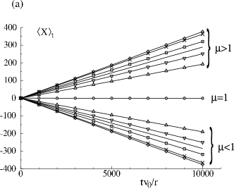
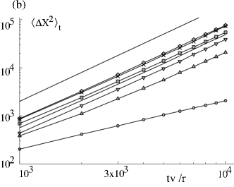
Figure 3: (a) Average horizontal position $\langle X\rangle_{t}$ in the billiard, as a function of time for different values of $\mu$. We see that for each value of $\mu$ there is a well defined slope (average velocity) and as $\mu$ increases so does the slope. (b) Plot of the mean square displacement $\langle\Delta X^{2}\rangle_{t}$, for the same values of $\mu$. We observe a clear quadratic behavior $\sim t^{2}$ (upper solid line) for all values of $\mu$, except for $\mu=1$ (lower curve) where the mean square displacement behaves linearly with time. For panel (a) the data corresponds to $\mu=1/1.53$ ($\triangledown$), 1/1.5 ($-$), 1/1.4 ($\times$), 1/1.3 ($\diamond$), 1/1.2 ($\square$), 1/1.1 ($\bigtriangleup$), 1 ($\circ$), 1.1 ($\bigtriangleup$), 1.2 ($\square$), 1.3 ($\diamond$), 1.4 ($\times$), 1.5 ($-$), 1.53 ($\triangledown$). Note that these values are chosen such that we have pairs $\mu$ and $1/\mu$. The symmetry $v\to-v$ when $\mu\to 1/\mu$ is seen in figure (a). In figure (b) the data for $\mu$ and $1/\mu$ almost superpose, thus we have plotted only values for $\mu\geq 1$. We recall the parameter values are $R/D=0.48$ and $r/D=0.395$.

For $\mu=1$ the chain is periodic and we know that the mean value stays constant (no drift) and the spreading of the density is that of a diffusive process. Thus the density for long times is distributed according to a Gaussian, with a variance growing as $\sqrt{t}$. This is confirmed by the numerical result shown in Fig. 3, central curve on panel (a) and bottom curve on panel (b).

For $\mu\neq 1$ we observe that the packet moves towards the region of growing size cells (i. e. to the left for $\mu<1$ and right for $\mu>1$). The velocity of this motion is obtained by computing the average position of the particles at different times, which is plotted in Fig. 3. Clearly there is a well defined constant speed for each value of $\mu$. This speed is plotted as a function of $\mu$ in Fig. 4. The data is plotted together with the speed, Eq. (35), obtained from a macroscopic model based on a master equation to be described in Sec. IV and a linear approximation for small values of $\mu-1$.

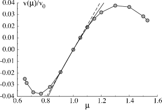
Figure 4: Dots: Plot of the velocity $v$ as a function of $\mu$. The solid line is the function $c(\mu-1/\mu)(\sqrt{\mu}+1/\sqrt{\mu})$, with $c=0.05$ a constant we use to fit the data close to $\mu=1$ (the reason to plot this function will become clear in Sec. IV). The dashed line is a straight line with slope 0.21. Note that for values of $\mu$ away from $\mu=1$ the dots are not well approximated by the line.

We also computed the mean square displacement $\Delta X^{2}=\langle X^{2}\rangle-\langle X\rangle^{2}$ as a function of time. The numerical observation, Fig. 3b is that $\Delta X^{2}\sim t^{2}$, i. e absence of diffusion, as expected from the macroscopic description of the system in Sec. IV.

III A self-similar Graph

In order to simplify matters a bit, we introduce a stochastic system in the form of a graph, with properties similar to the self-similar billiard described in the previous section. In a sense, this self-similar graph is an intermediate description between the billiard and a macroscopic description based on a Master equation, to be discussed in Sec. IV.

Graphs are geometrical objects made of vertices connected by bonds of given lengths, on which particles are allowed to move according to specific rules. The particles move freely on the bonds and get randomly scattered at the vertices to any of the connected bonds, according to prescribed transition probabilities. The classical dynamics of graphs share many properties of one-dimensional chaotic maps. in fact every graph can be mapped to an expanding one-dimensional map ClasGraph .

The model we consider is self-similar in the sense that the lengths of the bonds grow exponentially with their indices. Here the chaotic dynamics of the billiard is replaced by a one-dimensional free flight and a probabilistic law that determines the transition probabilities between cells.

III.1 Definition of the Model

The graph is defined as follows. It consists of a linear chain of bonds, connected to one another from end to end. Transition probabilities to the left, $T_{L}$, and to the right, $T_{R}$, are taken to scale according to $T_{R}/T_{L}=\mu$, with the parameter $\mu$ playing a role similar to the billiard’s. This choice is motivated by the dynamics of the billiard. Indeed, provided we can assume the escape probabilities are small, we expect trajectories to distribute uniformly within the cells before exiting, so that the escape probabilities to the left and right are within a ratio $\mu$ of one another. Thus let $T_{L}=p/\sqrt{\mu}$ the transition probability to the left, and $T_{R}=p\sqrt{\mu}$ to the right. Like in the billiard, we have a reference cell (with index zero) with a bond whose length we take to be $L_{0}$. The first cell to the right has length $L_{1}=L_{0}\mu$ and the $i$th cell to the right has length $L_{i}=L_{0}\mu^{i}$. Likewise the first cell to the left has length $L_{-1}=L_{0}\mu^{-1}$ and the $i$th cell to the left $L_{-i}=L_{0}\mu^{-i}$. The transition probabilities for all the cells are the same as for the zeroth cell and we take for left vertex transition $T_{L}$ and reflection $R_{L}=1-T_{L}$, and for the right vertex $T_{R}$ and reflection $R_{R}=1-T_{R}$.

Figure 5: Schematic representation of a self-similar graph with $\mu=2$.

III.2 Two Properties of the Spectrum of the self-similar Graph

We identify two properties of the spectrum of the Perron-Frobenius operator of the self-similar graph, analogous to Properties 1-2 for the billiard. The Perron-Frobenius operator and its spectral decomposition was studied in ClasGraph . Here we use the tools developed in that article. In particular, as explained in ClasGraph , the Pollicott-Ruelle spectrum $\{s_{i}\}$ for graphs is obtained by computing the zeros of the secular equation

$$\det[I-Q(s)]=0,$$ (15)

where, in the case that concerns us, the matrix $Q$ of the infinite system has elements $Q_{ab}=P_{ab}e^{sL_{b}}$, given by the probability of going from the bond $b$ to the bond $a$ times the exponential function involving the length $L_{b}$ of bond $b$. Here we must take the bonds to be directed, thus $b$ and $\hat{b}$ represent the same bond, but with opposite directions. In our case, the graph has a linear structure and only neighboring bonds are coupled. The matrix $Q$ is ordered in such a way that the column $a$ and row $b$ goes in order of increasing index, alternating directions, $\{\ldots,-1,\widehat{-1},0,\hat{0},1,\hat{1},\ldots\}$,

$$Q(s)=\left(\begin{array}[]{cccccc}\ddots&&T_{L}e^{sL_{1}}&&&\\ &0&R_{L}e^{sL_{1}}&0&0&\\ &R_{R}e^{sL_{1}}&0&0&T_{L}e^{sL_{2}}&\\ &T_{R}e^{sL_{1}}&0&0&R_{L}e^{sL_{2}}&\\ &0&0&R_{R}e^{sL_{2}}&0&\\ &&&T_{R}e^{sL_{2}}&&\ddots\end{array}\right)$$ (16)

From Eqs. (15)-(16), and from the definition of $L_{i}$, we infer the following property :

Property 3 (Analogous to property 1)

If $s_{0}$ is a solution of Eq. (15) then so is $s_{0}\mu$.

To see this, note that changing $s$ by $s\mu$ in Eq. (16) amounts to shifting the elements of the matrix by two rows downwards and two columns to the right, because it is equivalent to changing $L_{i}\to L_{i+1}$. Since the matrix is infinite, this change leaves $Q$ unchanged. Thus, if $s$ is a solution of the secular equation (15) then so is $s\mu$. Thus, given a solution $s_{0}$, we can identify a family of solutions $\{s_{i}\}_{-\infty}^{\infty}$ where each $s_{i}=s_{0}\mu^{i}$. Given a different solution $s^{\prime}_{0}$, there is another family $\{s^{\prime}_{i}\}_{-\infty}^{\infty}$.

For a given family of solutions, the ratio between to roots of Eq. (15) is an entire power of $\mu$. Roots from different families do not have this property.

Property 4 (Analogous to property 2)

If $\chi_{0}=\{\ldots,a_{-1}a_{\widehat{-1}},a_{0},a_{\hat{0}},a_{1},a_{\hat{1}},\ldots\}$ is the eigenvector associated to $s_{0}$, i. e. $Q(s_{0})\chi_{0}=\chi_{0}$, then the eigenvector associated to $s_{1}=s_{0}\mu$ is $\chi_{1}=\{\ldots,a_{0},a_{\hat{0}},a_{1},a_{\hat{1}},a_{2},a_{\hat{2}},\ldots\}$, whose elements are shifted to the left compared to $\chi_{0}$. That is, if $a_{i}$ is the $i$th element of $\chi_{0}$, then it is also the $(i-2)$th element of $\chi_{1}$ or in general $\chi_{j+1}[b]=\chi_{j}[b+2]$, which implies, $\chi_{j}[b]=\chi_{0}[b+2j]$.

With the same argument we have that the left eigenvector satisfies $\tilde{\chi}_{j+1}[b]=\tilde{\chi}_{j}[b+2]$.

Property 4 has a simple interpretation. First, note that due to the order we used for the matrix $Q$ a shift by two elements on the vectors corresponds to a shift by one cell on the chain. Therefore, property 4 says that, the mode $\chi_{j+1}$ is equal to the mode $\chi_{j}$, but shifted to the left by one cell. And property 3 says that the mode $\chi_{j+1}$ has a lifetime which is a factor $1/\mu$ shorter, if $\mu>1$, (resp. longer if $\mu<1$) than the lifetime of the mode $\chi_{j}$. Thus the spectrum of the evolution operator of the graph has the same properties as the spectrum of the evolution operator of the billiard.

III.3 From the Spectrum of self-similar Systems to the Drift

As was shown in numerical simulations of particles moving in the billiard in Sec. II.5, a density of particles drifts towards the regions of growing cell size of the chain with a constant velocity, while at the same time it spreads ballistically. We will show shortly this also holds for the graph.

A heuristic justification for the constant drift can be given thanks to the self-similar structure of the system as follows. Anywhere in the system, the probability is greater for particles to exit in the direction of increasing scales. Furthermore as the scales grow, the average time a particle spends in a cell increases accordingly. Hence we expect the drift to remain constant.

Now we offer a quantitative analysis of the drift, based upon properties 1 and 2, or, equivalently, 3 and 4.

The spectral decomposition of the Perron-Frobenius operator $\widehat{P}^{t}$ was obtained in thomas ; ClasGraph for graphs and in GaspB ; Gas96 for billiards. For graphs, the time evolution of an observable $A[b,x_{b}]$ has the asymptotic expression ($t\to\infty$)

$$\langle A\rangle_{t}=\langle A|\widehat{P}^{t}\rho_{0}\rangle=\sum_{j}\langle A|\psi_{j}\rangle e^{s_{j}t}\langle\tilde{\psi_{j}}|\rho_{0}\rangle+\ldots$$ (17)

with

$$\langle A|\psi_{j}\rangle = \sum_{b^{\prime}=-\infty}^{\infty}\chi_{j}[b^{\prime}]\frac{1}{l_{b^{\prime}}}\int_{0}^{l_{b^{\prime}}}e^{-s_{j}x/v}A[b^{\prime},x]dx,$$ (18)

$$\langle\tilde{\psi_{j}}|\rho_{0}\rangle = \frac{1}{N_{j}}\sum_{b^{\prime}=-\infty}^{\infty}\tilde{\chi}_{j}[b^{\prime}]\int_{0}^{l_{b^{\prime}}}e^{s_{j}x/v}\rho_{0}[b^{\prime},x]dx,$$ (19)

and

$$N_{j}=\sum_{b}l_{b}\tilde{\chi}_{j}[b]^{*}\chi_{j}[b].$$ (20)

In Eq. (17) the dots stand for terms whose coefficients carry subexponential time dependence which may arise from degeneracies of the spectrum and can be neglected in the long time limit. Similar expressions can be obtained for billiards with the same conclusion GaspB ; Gas96 , however for the sake of simplicity we will state the results for graphs only.

We assume the initial density to be localized on one bond, namely $\rho_{t=0}[b,x_{b}]=\delta_{b,b_{0}}\delta(x_{b}-x_{0})$, i. e. all the particles start from $x_{0}$ on the bond $b_{0}$. To simplify as much as possible the calculation and notation we will consider $x_{0}=0$ and the bond $b_{0}$ as the reference bond $b_{0}=0$. We are interested in the density as a function of the position and $t$, i.  e. $\rho_{t}[b,x_{b}]$, so we define the observable $A$ by $A[b^{\prime},x_{b^{\prime}}]=\delta_{b,b^{\prime}}\delta(x_{b}-x_{b^{\prime}})$, in such a way that $\langle A\rangle_{t}=\rho_{t}[b,x_{b}]$, as we see from Eq. (17). For simplicity, we also take $x_{b}=0$, i. e. we measure the density at the beginning of the bond $b$.

Using this in Eq. (17), Eq. (19) and Eq. (20) we get

$$\langle A\rangle_{t}=\sum_{j}\chi_{j}[b]\frac{e^{s_{j}t}}{N_{j}l_{b}}\tilde{\chi}_{j}[0].$$ (21)

Now, since the spectrum is divided in families according to whether or not $s_{j}/s_{k}$ is an entire power of $\mu$, let us consider the contribution of only one of these families to the sum in Eq. (21).

From property 4, if $\chi_{j}[b]$ is the eigenstate associated to $s_{j}$ then, the eigenstate associated to $s_{j}/\mu$ is $\chi_{j-1}[b]=\chi_{j}[b-2]$ and corresponds to the state $\chi_{j}$ but shifted one cell to the right. It is then easy to see that $N_{j}=\mu^{-2j}N_{0}$.

Moreover, from Property 3, we have that if $s_{0}$ is a decay rate (Pollicott-Ruelle resonance), then there is a family of Pollicott-Ruelle resonances associated to it given by $s_{j}=s_{0}\mu^{j}$.

Now using the expressions of the lengths $L_{b}=L_{0}\mu^{b}$, we have that the contribution to Eq. (21) due to this familiy is

$$\frac{1}{N_{0}}\sum_{j=-\infty}^{\infty}\chi_{j}[b]\frac{\mu^{2j}}{\mu^{b}}e^{s_{0}\mu^{j}t}\tilde{\chi}_{j}[0]$$ (22)

Let us split this sum in two parts, first the terms with $j=-\infty,\ldots,0$ and second $j=1,\ldots,\infty$. We consider for now the first term only, i. e. $j=0,-1,\dots,-\infty$.

1. For $j=0,-1,\dots,-\infty$, $s_{0}$ is the largest decay rate. Therefore the component with the corresponding rate, $\chi_{0}$, is the first to decay. After it has decayed, the part of the density represented by this part of the sum –which we refer to as the density for short– moves to the right, because, as a consequence of property 4, all the other modes are shifted to the right of $\chi_{0}$.

2. The support of the density is shifted to the right by a distance $L$, corresponding to the length of the bond where the mode $\chi_{0}$ is centered. Let us call it $b_{c}$.

3. Then, the component of the mode $\chi_{-1}$ is the second to decay with a rate $s_{0}/\mu$ and the support of the density moves another bond to the right because, by property 4, the bond where the mode $\chi_{-1}$ is centered is the one at the right of $b_{c}$, i. e. it is the bond $b_{c+1}$. This bond $b_{c+1}$ is larger by a factor $\mu$ than $b_{c}$.

Thus if we take the distance the packet moves divided by the characteristic time (given by the inverse of the decay-rate), we have that, during the decay time of the first mode, the speed was $Ls_{0}$ and, during the decay time of the second mode to decay, the speed was $(L\mu)s_{0}/\mu=Ls_{0}$, equal to the first. We can obtain the same result for the decay of the third mode, $(L\mu^{2})s_{0}/\mu^{2}=Ls_{0}$, and so on.

Now, it is clear that the same conclusion follows from the other terms $j=1,\ldots,\infty$ of the sum, thus we conclude the packet moves at a constant speed.

This argument shows that a constant drift of particles has to be expected in the self-similar systems as defined here.

If we were able to obtain the exact eigenvectors we could compute numerically this sum and compare with simulations. Instead we propose a heuristic argument and assume the eigenvectors are localized around some finite region of the chain. A simple possibility is to assume a Gaussian shape for the left and right eigenvectors, satisfying property 4, namely $\chi_{j}[b]=\tilde{\chi}_{j}[b]=\exp[\frac{-(b-(b_{0}-2j))^{2}}{\sigma^{2}}]$. The argument that the eigenvectors are localized can be justified with a perturbative calculation provided the transmission probability $p\ll 1$, similar to thomas .

For this heuristic calculation, we consider values of $\mu$ close to one, so we write $\mu=1+\epsilon$ and we can compute the sum in Eq. (22) for small $\epsilon$. We also do the change of variable (we take $L_{0}=1$) $y=\frac{\mu^{b}-1}{\mu-1}\Rightarrow b\approx y+\epsilon y^{2}/2$ which measures the distance from the origin to the bond $b$. Then we obtain

$$\langle A\rangle\sim\exp[-\frac{y^{2}}{2\sigma^{2}}-\epsilon\frac{y^{3}}{2\sigma^{2}}+s_{0}t(1-\epsilon y/4)-\frac{3y\epsilon}{2}]$$ (23)

Now, we calculate the position of the maximum of Eq. (23) as a function of $t$ and obtain

$$y_{m}\approx-\epsilon\frac{\sigma^{2}}{2}(s_{0}t/2+3)$$ (24)

We have a maximum that is linear in $\mu-1$, moves in the appropriate direction and is zero if $\mu=1$, in agreement with simulations to be presented next. Thus we have shown that the two properties of the spectrum are related to the motion of the packet. It will be desirable to have a similar understanding of the spreading of the density in terms of the spectrum of the Liouvillian operator.

III.4 Transport Properties of the self-similar Graph: Numerical Results

The evolution of a density of particles in this system behaves in a way similar to the billiard chain. As with the billiard, a well-defined constant drift is observed, as shown in Fig. 6 (a). The dependence of this drift in $\mu$ is depicted in Fig. 7. Here we also observe that the mean square displacement $\Delta X^{2}=\langle X^{2}\rangle-\langle X\rangle^{2}$ as a function of time, Fig. 6 (b), behave like $\Delta X^{2}\sim t^{2}$. This ballistic spreading of the density is also found with the macroscopic description of the system as given in Sec. IV.

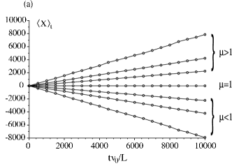
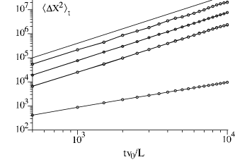
Figure 6: (a) Average horizontal position $\langle X\rangle_{t}$ in the graph vs. time, for different values of $\mu$. We see that for each value of $\mu$ there is a well defined slope (velocity) and as $\mu$ increases so does the slope. (b) Mean square displacement $\langle\Delta X^{2}\rangle_{t}$, for the same values of $\mu$. We observe a clear $\sim t^{2}$ (upper line) for all values of $\mu$ except for $\mu=1$ (lower curve) where the behavior is $\sim t$. The same values of $\mu$ as in Fig. 3 were used.

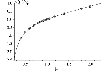
Figure 7: Plot of the velocity $v$ as a function of $\mu$. The line is the function $c(\mu-1/\mu)(\sqrt{\mu}+1/\sqrt{\mu})$, with $c$ a constant we use to fit the data. The reason to plot this function will become clear in Sec. IV

IV Macroscopic description

In this section we present a system which is a charicature of the self-similar systems considered so far and helps understand the macroscopic evolution on systems with self-similar structure. It describes the dynamics based on a Master equation approach Hanson . For this model we are able to obtain analytical expressions for the (constant) drift velocity and the ballistic spreading of the density.

We consider a discrete sequence of states $i\in\mathbb{Z}$ and, associated to them, we have a conditional probability $P_{i}(t)$ which represents the probability of being at site $i$ at time $t$ given some initial condition to be specified later. We will identify the sequence of sites with the sequence of cells of the billiard or graph. Since for the billiard and graph only transitions to neighboring cells are allowed, we introduce the transition rates $W^{-}_{i}$ and $W^{+}_{i}$, respectively for transitions to the left and to the right of the site $i$. The master equation rules the time evolution of the $P_{i}(t)$ and for this process it has the form

$$\partial_{t}P_{i}(t)=P_{i+1}(t)W^{-}_{i+1}+P_{i-1}(t)W^{+}_{i-1}-P_{i}(t)(W^{+}_{i}+W^{-}_{i}),$$ (25)

It is a gain-loose or balance equation. To mimic the transitions that occur on the graph, we consider $W^{-}_{i}$ (respectively $W^{+}_{i}$) as the ratio between the probability of going to the left, i. e. $p/\sqrt{\mu}$ (respectively $p\sqrt{\mu}$ for the right) over the characteristic time associated to bond $i$ $L_{0}\mu^{i}/v_{0}$, i. e.,

$$W^{-}_{i} = \frac{pv_{0}}{L_{0}}\mu^{-i-1/2},$$ (26)

$$W^{+}_{i} = \frac{pv_{0}}{L_{0}}\mu^{1/2-i}.$$ (27)

Thus Eq. (25) becomes

$$\partial_{t}P_{i}(t)=\frac{pv_{0}}{L_{0}}\mu^{-i}\left[\mu^{-3/2}P_{i+1}(t)+\mu^{3/2}P_{i-1}(t)-(\mu^{1/2}+\mu^{-1/2})P_{i}(t)\right].$$ (28)

In matrix notation, this reads

$$\partial_{t}P_{i}(t)=\mathcal{L}_{ij}P_{j}(t)\ ,$$ (29)

where

$$\mathcal{L}_{ij}=\frac{pv_{0}}{L_{0}}\mu^{-j}[\mu^{-1/2}\delta_{j,i+1}+\mu^{1/2}\delta_{j,i-1}-(\mu^{1/2}+\mu^{-1/2})\delta_{ij}].$$ (30)

By exponentiation, since $P_{j}(t=0)=\delta_{j0}$,

$$P_{i}(t)=\exp[\mathcal{L}t]_{ij}\delta_{j0}$$ (31)

Note the symmetry of $\mathcal{L}$, $\mathcal{L}_{ij}(\mu)=\mathcal{L}_{-ji}(1/\mu)$, implies $P_{i}(t)\to P_{-i}(t)$ upon inverting $\mu$.

Note that until here, the model does not contain any metric information. Only part of the self-similar structure is introduced through the transition rates $W^{\pm}_{i}$. The geometrical part of the self-similar structure is implemented by associating a quantity $X_{i}$ to each site $i$ which is a measure of the distance from the origin to the site $i$. We define it following the geometry of the graph. If the site $i=0$ corresponds to the bond of length $L_{0}$, and the site $i$ to the bond of length $L_{i}=L_{0}\mu^{i}$, $X_{i}$ measures the distance from the middle of the $i$th bond to the middle of the $0$th bond (i. e. the origin), viz.

$$X_{i}(\mu)=\frac{L_{0}(1-\mu^{i})}{2}\frac{1+\mu}{1-\mu}.$$ (32)

In the expressions on the RHS, we observe the symmetry $X_{i}\to-X_{-i}$ under the change $\mu\to 1/\mu$. In other words $X_{i}(1/\mu)=-X_{-i}(\mu)$.

We define the average position at time $t$ by

$$\langle X\rangle_{t}=\sum_{i}P_{i}(t)X_{i},$$ (33)

The velocity is defined by

$$V(t)=\partial_{t}\langle X\rangle_{t}=\sum_{ij}\mathcal{L}_{ij}P_{j}(t)X_{i}.$$ (34)

According to the symmetries above, we should have $V\to-V$ upon inverting $\mu$, which we can check by direct calculation. We have

$$V(t) = \frac{pv_{0}}{L_{0}}\sum_{j}\mu^{-j}P_{j}[\mu^{-1/2}X_{j-1}+\mu^{1/2}X_{j+1}-(\mu^{-1/2}+\mu^{1/2})X_{j}],$$

$$= \frac{pv_{0}}{L_{0}}\sum_{j}\mu^{-j}P_{j}[\mu^{-1/2}(X_{j-1}-X_{j})+\mu^{1/2}(X_{j+1}-X_{j})]\ .$$

Using Eq. (32), we obtain the expression

$$V(t)=\frac{pv_{0}}{2}(\mu-\mu^{-1})(\mu^{-1/2}+\mu^{1/2}).$$ (35)

We observe that the speed has a constant value which vanishes for $\mu=1$ as expected. Moreover it is clearly anti-symmetric upon inverting $\mu$.

Now we evaluate the time derivative of the mean square displacement,

$$\partial_{t}\langle\Delta X^{2}\rangle\equiv\partial_{t}[\langle X^{2}\rangle_{t}-\langle X\rangle_{t}^{2}]=\partial_{t}\langle X^{2}\rangle_{t}-2\langle X\rangle_{t}\partial_{t}\langle X\rangle_{t}.$$ (36)

with $\langle X^{2}\rangle_{t}=\sum_{i}P_{i}(t)X_{i}^{2}$. Eq. (36) can be written as

$$\partial_{t}\langle\Delta X^{2}\rangle=\sum_{ij}\mathcal{L}_{ij}P_{j}(t)X_{i}[X_{i}-2\langle X\rangle_{t}].$$ (37)

replacing $\mathcal{L}$ given in Eq. (30) in Eq. (37) we get

$$\partial_{t}\langle\Delta X^{2}\rangle = \frac{pv_{0}}{L_{0}}\sum_{ij}\mu^{-j}P_{j}(t)[\mu^{-1/2}(X_{j-1}-X_{j})(X_{j}+X_{j-1}-2\langle X_{t}\rangle)+\mu^{1/2}(X_{j+1}-X_{j})(X_{j+1}+X_{j}-2\langle X_{t}\rangle)],$$ (38)

$$= \frac{pv_{0}}{L_{0}}\left(\mu\sqrt{\mu}+\frac{1}{\mu\sqrt{\mu}}\right)\left[\left(\frac{L_{0}}{2}\left(\sqrt{\mu}+\frac{1}{\sqrt{\mu}}\right)\right)^{2}+\frac{v_{0}t}{2\sqrt{\mu}}\left(\mu-\frac{1}{\mu}\right)^{2}\right],$$

where we used Eq. (32) and the fact that $\langle X_{t}\rangle=Vt$.

In the long time limit, i. e. $t\gg t_{c}=\frac{L_{0}}{2v_{0}}\frac{\mu\sqrt{\mu}}{\mu-1}$, we can neglect the constant term and therefore $\Delta X^{2}\equiv\langle X^{2}\rangle_{t}-\langle X\rangle_{t}^{2}\sim t^{2}$. In other words, the spreading of the density is ballistic, similar to what we observed numerically in the billiard and graph. In the opposite case $t\ll t_{c}$ the constant term dominates in $\partial_{t}\langle\Delta X^{2}\rangle$ and the spreading is diffusive. The time $t_{c}=\frac{L_{0}}{2v_{0}}\frac{\mu\sqrt{\mu}}{\mu-1}$, marks the crossover from diffusive to ballistic behavior of the mean-square displacement.

Let us compare the speed, Eq. (35), obtained in this macroscopic model with the numerical results of sections II.5 and III.4. In the case of the billiard (see figure 4), the agreement is poor, because the Master equation is not a good model for the billiard, except perhaps for $\mu\approx 1$. In fact, a particle in a given cell of the billiard escapes easily in a few collisions and thus we do not expect that the master equation, where the cell has a uniform probability, will be a good quantitative model. On the other hand what is observed is that for values of $\mu\approx 1$ the speed is proportional to $\mu-1$. In the case of the graph, see figure 7, Eq. (35) fits very well the data because the probability of being in a bond is well approximated by a uniform distribution in the limit $p\ll 1$ where many collisions occurs in average with the scatterers before the particle goes to another bond. Thus we expect the master equation to be a good model for this system.

Finally we show that for this macroscopic description, we also have properties similar to 1 and 2 (or 3 and 4), and therefore a correspondence between the constant drift and the spectral properties of $\mathcal{L}$.

The decay rates can be computed assuming a solution of the form $P_{i}(t)=e^{st}Q_{i}$ . Upon substitution of this expression into Eq. (29), we find that the decay rates $s$ must be solutions of

$$\det[s\delta_{ij}-\mathcal{L}_{ij}]=0\ .$$ (39)

Now we proceed as with the billiard and the graph. We assume a particular solution $s$ of Eq. (39) was obtained and analyze $\det[s\mu\delta_{ij}-\mathcal{L}_{ij}]$. Note that due to the definition of $\mathcal{L}$ we have $\mathcal{L}_{i,j}=\mu\mathcal{L}_{i+1,j+1}$. Therefore,

$$\det[s\mu\delta_{ij}-\mathcal{L}_{ij}]=\det[\mu(s\delta_{i+1,j+1}-\mathcal{L}_{i+1,j+1})]\ .$$ (40)

Because $\mu\neq 0$, we conclude that if $s$ is a solution of Eq. (39) then so is $s\mu$.

Now, the associated eigenvector $Q^{s}_{i}$ is obtained from $\sum_{j}[s\delta_{ij}-\mathcal{L}_{ij}]Q^{s}_{j}=0$ and $Q^{s\mu}_{i}$ is obtained from $\sum_{j}[s\mu\delta_{ij}-\mathcal{L}_{ij}]Q^{s\mu}_{j}=0$. Again, using the definition of $\mathcal{L}$, it is easy to show that $Q^{s\mu}_{i}=Q^{s}_{i+1}$. This shows we have again the equivalent of properties 1 and 2 (or 3 and 4).

V conclusions

In this article we have studied the statistical properties of three different classes of self-similar systems and found that all three share very similar macroscopic properties; we observe a drift of particle densities towards the direction of growing scales at constant velocity, as well as a ballistic spreading of the density.

A justification for the presence of a drift was provided, for both the billiard chains and graphs, in terms of two essential properties of the spectrum of the evolution operator, the first stating that for every decay-rate $s$, there is also a decay rate $s\mu$, and, correspondingly, the second, that the eigenstate associated to $s\mu$ is shifted one cell to the left of the chain with respect to the eigenstate associated to $s$.

As of the Billiard, we should note that these properties hold independently of the exact shape of the unit cell; they are merely a consequence of the self-similar structure. The only relevant restriction regarding the shape of the unit cell is that the dynamics in that billiard cell must be strongly chaotic in order to have the kind of spectral decomposition that we assumed.

For the self-similar graph, these properties are also rather general. Here we considered a very simple self-similar graph, to avoid complicated expressions, but we can take a unit cell composed of any number of bonds, say $N_{B}$, and by ordering the matrix $Q$ in such a way that all the bonds of the same cell are consecutive we will obtain property 3 and property 4, which will look like $\chi_{j+1}[b]=\chi_{j}[b+2N_{B}]$.

Let us discuss an interpretation of these two properties in term of periodic orbits. Consider the billiard. Decay rates and eigenstates are determined by an ensemble of periodic orbits that form a repellor Gas96 . Every periodic orbit can be shifted by one cell to the right or to the left and generate a new periodic orbit with the only difference that the period is a factor of $\mu$ respectively shorter or longer. If the periodic orbits determine the support of the eigenstates, then it is clear that eigenstates of the same ”shape” but shifted along the billiard exist and that the associated decay rates will also differ by a factor of $\mu$. The change in period (time scale) corresponds to property 1 and the fact that the geometry of the orbits is unchanged to property 2.

We have also provided a macroscopic description of self-similar billiards and graphs in terms of a Master Equation, for which we obtained an analytical expression of the velocity and ballistic spreading. Properties equivalent to 1 and 2 are also shared by this system.

We note that in going from the billiard to the graph and then to the Master Equation, the stochasticity increases. Billiards are deterministic chaotic systems; in graphs, there is a stochastic element which acts only when the particles reach the vertices, while the motion within the bond is deterministic; The dynamics described by the Master Equation is completely stochastic with transitions possibly occuring at any time.

We should also note that the existence of a drift is rather intuitive and simple to explain qualitatively in terms of the probabilities of crossing to the left or right and in terms of the time spent in the bigger or smaller cells. However, our aim was to provide an example where a macroscopic property like the drift of particles can be related to the microscopic properties of the system, i. e. the exact Liouvillian evolution operator.

Several perspectives are open for future research, of which we now mention two. First, it will be interesting to characterize the spreading in terms of properties of the spectrum and, second, regarding the billiard, we would like to obtain further understanding of the function $v(\mu)$. Our main observation of this work is that there is a well-defined speed of propagation for each value of $\mu$. However, a determination of the speed $v$ vs. $\mu$ is missing thus far. Numerical results (not all presented here) show that, as we change the parameters of the billiard, the speed displays a rich behavior as a function of $\mu$. For instance, we observed functions $v(\mu)$ that are monotonous with $\mu$ in some parameter regions, while in other regions, such as corresponding to the parameter values used in Fig. 4 we observed a non-monotonous function. Near $\mu=1$ the behavior of $v(\mu)$ is determined by the symmetry $v(\mu)=-v(1/\mu)$. In fact, it follows from that symmetry, that for small values of $\mu-1$, we can expand $v(\mu)=v^{\prime}(1)(\mu-1-(\mu-1)^{2}/2)+\ldots$

We expect to continue our work in these directions. In particular, we believe a better understanding of the dynamical system in the unit cell with boundary conditions given by Table 1 is needed, specifically regarding the properties of the invariant measure. Because of the open boundary condition, the invariant measure is not the Liouville measure. The volumes are not conserved by the matching conditions. One therefore expects fractal properties of the invariant measure. This will be the subject of further publications.

Appendix A Finite Horizon self-similar Billiard Channel

In this appendix, we extend the finite horizon condition for the usual periodic Lorentz gas to the self-similar case, so as to ensure hyperbolicity of the dynamics.

In the absence of self-similar structure ($\mu=1$), the Lorentz channel GaspB has the symmetry of a two-dimensional periodic Lorentz gas on a hexagonal lattice. This system is diffusive provided it verifies the so-called finite horizon conditions, namely

$$2R<D<4R/\sqrt{3},$$ (41)

where $R$ denotes the common radius of the scatterering disks and $D$ the distance between neighboring disks. The lower bound ensures that the disks do not overlap and the upper one that there are no free flying trajectories.

For a mixed Lorentz gas, with alternating rows of scatterers of radii $r$ and $R$, the hexagonal structure of the lattice is preserved, but the corresponding channel now consists of three rows of scatterers : the upper and lower rows with half disks of radii $R$ and the middle row with disks of radii $r$. The corresponding unit cell has a rectangular shape with four quarter disks of radii $R$ at the corners and one disk of radius $r$ at the center (where the diagonals intersect), with coordinates

$$4\ \mathrm{disks}\ \mathrm{of}\ \mathrm{radii}\ R : \begin{array}[]{l}\big{(}0,\pm\sqrt{3}D/2\big{)},\\ \big{(}D,\pm\sqrt{3}D/2\big{)},\end{array}$$ (44)

$$1\ \mathrm{disk}\ \mathrm{of}\ \mathrm{radius}\ r : (D/2,0).$$ (45)

For this system, the finite horizon conditions become

$$D > 2r,$$ (46)

$$D > 2R,$$ (47)

$$D < 2(r+R)/\sqrt{3}.$$ (48)

Now introducing the parameter $\mu$, we deform the cell of the Lorentz channel from a rectangle to a trapezoid with vertical sides scaled by $1/\sqrt{\mu}$ and $\sqrt{\mu}$ respectively, as was shown in Fig. 1. The positions of the disks become

$$4\ \mathrm{disks}\ \mathrm{of}\ \mathrm{radii}\ R : \begin{array}[]{l}\big{(}0,\pm\sqrt{3}D/(2\sqrt{\mu})\big{)},\\ \big{(}D,\pm\sqrt{3}D\sqrt{\mu}/2\big{)},\end{array}$$ (51)

$$1\ \mathrm{disk}\ \mathrm{of}\ \mathrm{radius}\ r : (D/(1+\mu),0),$$ (52)

where the disk on the horizontal axis lies at the intersection of the diagonals.

Let us assume $\mu>1$ in the sequel.

A.1 Non-Overlapping Disks

The non-overlapping conditions Eqs. (46-47) transpose to three new conditions :

1. The sum of the radii of the external disks must be less than the length of the lower/upper side of the cell,

   $$\frac{R}{\sqrt{\mu}}+\sqrt{\mu}R < \sqrt{D^{2}+\left[\frac{\sqrt{3\mu}D}{2}-\frac{\sqrt{3}D}{2\sqrt{\mu}}\right]^{2}},$$ (53)

   $$= D\sqrt{\frac{3}{4}(\mu+\mu^{-1})-\frac{1}{2}}.$$

2. The shortest diagonal must be greater than the sum of the radii $R/\sqrt{\mu}$ and $r$,

   $$\frac{R}{\sqrt{\mu}}+r<\sqrt{\left(\frac{\sqrt{3}D}{2\sqrt{\mu}}\right)^{2}+\left(\frac{D}{\mu+1}\right)^{2}}.$$ (54)

3. The radius of the center disk must be less than the distance from the intersection of the diagonal to the cell’s boundary. That is,

   $$r<\frac{D}{1+\mu}.$$ (55)

Let $\rho\equiv R/D$ and $\lambda\equiv r/D$ be two dimensionless parameters. The first of the three conditions above, Eq. (53), can be transformed into a second degree polynomial in $\rho$ :

$$(3/4-\rho^{2})\mu^{2}-(1/2+2\rho^{2})\mu+(3/4-\rho^{2})>0.$$ (56)

We must assume

$$\rho<\frac{\sqrt{3}}{2}.$$ (57)

The two roots of Eq. (56) are

$$\mu_{\pm}=\frac{1+4\rho^{2}\pm 2\sqrt{8\rho^{2}-2}}{3-4\rho^{2}},$$ (58)

which are real if $\rho\geq 1/2$. In this case, the condition (53) is only satisfied provided either of

$$\begin{array}[]{c}\mu>\mu_{+},\mu<\mu_{-},\end{array}$$ (59)

hold. Note that $\mu_{+}=1/\mu_{-}$. These conditions are depicted in Fig. 8.

Otherwise, if $\rho<1/2$, Eq. (56) has no real roots and Eq. (53) is always true.

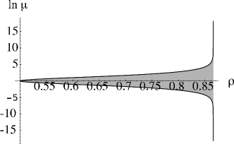
Figure 8: From Eqs. (58, 59). The gray region is forbidden when $1/2<\rho<\sqrt{3}/2$.

Consider the second condition, Eq. (54), which takes the form

$$\left[\frac{3}{4}-(\rho+\lambda\sqrt{\mu})^{2}\right](\mu+1)^{2}+\mu>0.$$ (60)

This is a sixth order polynomial in $\sqrt{\mu}$, with potentially as many roots, but is easy to solve numerically.

With these notations, we rewrite Eq. (55) as

$$\mu<\frac{1}{\lambda}-1.$$ (61)

A.2 Finite Horizon

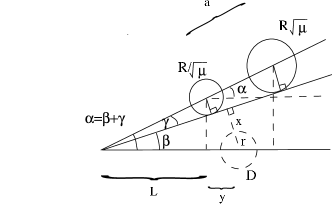
Figure 9: Geometry and definition of $\alpha,\beta,\gamma$ and $x$

The condition that there are no free-flying trajectories, as seen in Fig. 9, is that the line tangeant to the row of upper disks intersect the disk at the center.

Consider the reference cell and let $x$ denote the distance from the center of the central disk to the trajectory tangent to the upper disks. Since these lines are perpendicular, we can write

$$x=(L+y)\sin\beta,$$ (62)

where $y=D/(\mu+1)$ is the distance from the boundary of the cell to the center of the disk and $L=D\sum_{-\infty}^{-1}\mu^{i}=D/(\mu-1)$. In order to compute the angle $\beta$, we write $\beta=\alpha-\gamma$, where $\alpha$ and $\gamma$ are given as follows.

First we have that the difference between the two verticals from the base line to the upper right and upper left disks is $\sqrt{3}/(2D)(\sqrt{\mu}-1/\sqrt{\mu})$ and $D$ is the horizontal distance between their centers. Therefore

$$\tan\alpha=\frac{\sqrt{3}}{2}\left(\sqrt{\mu}-\frac{1}{\sqrt{\mu}}\right)$$ (63)

We note that the distance $a$ along the wall is given by

$$a = D/\cos\alpha,$$ (64)

$$= \frac{D}{2}\sqrt{3(\mu+\mu^{-1})-2}.$$

We can then compute $\gamma$ from the equality

$$\sin\gamma = \frac{R/\sqrt{\mu}}{a\sum_{-\infty}^{-1}\mu^{i}},$$ (65)

$$= \frac{R(\mu-1)}{a\sqrt{\mu}},$$

$$= \frac{2R}{D}\frac{\mu-1}{\sqrt{3\mu^{2}-2\mu+3}}.$$

Now, since $\beta=\alpha-\gamma$ we have

$$\sin\beta = \sin\alpha\cos\gamma-\cos\alpha\sin\gamma,$$

$$= \frac{2\rho\sqrt{\mu}(\mu-1)}{3-2\mu+3\mu^{2}}$$

$$\times\left[\sqrt{\frac{3}{\mu}\left[\frac{3-2\mu+3\mu^{2}}{4\rho^{2}}-(\mu-1)^{2}\right]}-2\right].$$

The finite horizon condition is

$$\lambda=\frac{r}{D}>\frac{2\mu}{\mu^{2}-1}\sin\beta.$$ (67)

In the limit $\mu\to 1$ one retrieves Eq. (48).

A.3 Choice of Parameter values

We want to fix the values of $\rho=R/D$ and $\lambda=r/D$ and find the range of values of $\mu$ so as to verify the constraints specified by Eqs. (53, 54, 55, 67).

The numerical results presented in Sec. II.5 use the fixed parameters $\lambda=r/D=0.395$ and $\rho=R/D=0.480$. For those values, the range of allowed values of $\mu$ is $0.653\leq\mu\leq 1.532$. For the sake of illustration, other possible parameter values are shown in Figs. 10-11 with either $\rho$ or $\lambda$ fixed.

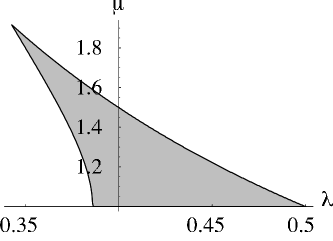
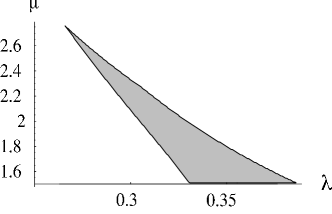
Figure 10: Values of $\mu$ vs. $\lambda$, for fixed $\rho$ = 0.48 (a), 0.52 (b), which are consistent with Eqs. (53), (54), (55) and (67).

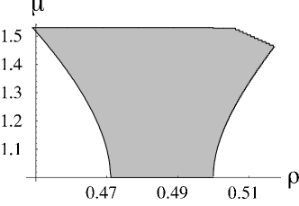
Figure 11: Values of $\mu$ vs. $\rho$, for fixed $\lambda$ = 0.395 which are consistent with Eqs. (53), (54), (55) and (67).

Appendix B Alternative proof of properties 1 and 2 for a self-similar billiard

The dynamics in the billiard chain is Hamiltonian and therefore the Liouville measure is invariant under the time evolution. According to Birkhoff, the Liouville measure can be expressed as $d\zeta d\tau$, where $\zeta=(s,v_{\mathrm{t}})$ is a pair of variables with $s$ representing the arc-length of the billiard (not the unit cell), and $v_{\mathrm{t}}$ the projection of the velocity to the tangential direction at the point $s$. Because the energy is conserved we can fix the speed $|v|=1$. With this choice $-1<v_{\mathrm{t}}<1$. Now, $\tau$ is a variable which measures a distance along a line drawn from the point $s$ with the direction given by $v_{\mathrm{t}}$. Obviously, $\tau$ can vary from zero to the intersection of this line with the billiard. This distance will be denoted by $T(\zeta)$, i. e. $0<\tau<T(\zeta)$. Thus we can consider that the average of a function $f(\zeta,\tau)$ is given by

$$\langle f\rangle=\frac{1}{\int ds\int dv_{\mathrm{t}}\int_{0}^{T(\zeta)}d\tau}\int ds\int dv_{\mathrm{t}}\int_{0}^{T(\zeta)}d\tau f(s,v_{\mathrm{t}},\tau).$$ (68)

The variable $s$ is unbounded because the billiard is infinite. Due to the construction of our billiard, we can split the integral over the arc-length into the contributions over the differents cells, i. e.

$$\int ds=\sum_{I}\int_{0}^{L_{I}}ds\ .$$ (69)

Due to the symmetry $L_{I}=\mu^{I}L_{0}$, we can let $0<s<L_{0}$. The restriction of the variable $\zeta$ to this region will be called $\xi$. We also observe that $T(\zeta)=T(\xi,I)=L(\xi)\mu^{I}$. Thus the average can be written as

$$\langle f\rangle=\frac{1}{\sum_{I}\mu^{I}\int ds\int dv_{\mathrm{t}}\int_{0}^{T(\xi,I)}d\tau}\sum_{I}\mu^{I}\int_{0}^{L_{0}}ds\int dv_{\mathrm{t}}\int_{0}^{T(\xi,I)}d\tau f(s,v_{\mathrm{t}},\tau,I),$$ (70)

or, in a more compact form, using $\int d\xi T(\xi,I)=\mu^{I}\langle L(\xi)\rangle$,

$$\langle f\rangle=\lim_{J\to\infty}\frac{1}{\sum_{I=-J}^{J}\mu^{2I}\langle L(\xi)\rangle}\sum_{I=-J}^{J}\mu^{I}\int d\xi\int_{0}^{T(\xi,I)}d\tau f(\xi,\tau,I).$$ (71)

Now, the quantity that is of interest to us is

$$\langle\tilde{b}_{s^{*}}b_{s}\rangle = \lim_{J\to\infty}\frac{1}{\sum_{I=-J}^{J}\mu^{2I}\langle L(\xi)\rangle}\sum_{I=-J}^{J}\mu^{I}\int d\xi\int_{0}^{T(\xi,I)}d\tau\tilde{b}_{s^{*}}(\xi,I)b_{s}[\xi,I],$$ (72)

$$= \lim_{J\to\infty}\frac{1}{\sum_{I=-J}^{J}\mu^{2I}\langle L(\xi)\rangle}\sum_{I=-J}^{J}\mu^{2I}\int d\xi L(\xi)\tilde{b}_{s^{*}}(\xi,I)b_{s}[\xi,I].$$

We assume that $s$ is a resonance i. e., $\langle\tilde{b}_{s^{*}}b_{s}\rangle=1$ Gas96 and we want to show that this implies $\langle\tilde{b}_{\mu s^{*}}b_{\mu s}\rangle=1$, that is that $s\mu$ is also a resonance.

To show this, we note that, from the formal expression of $b_{s}$, we have $b_{\mu s}[\xi,I]=b_{s}[\xi,I+1]$, and therefore

$$\langle\tilde{b}_{\mu s^{*}}b_{\mu s}\rangle=\lim_{J\to\infty}\frac{1}{\sum_{I=-J}^{J}\mu^{2I}\langle L(\xi)\rangle}\sum_{I=-J}^{J}\mu^{2I}\int d\xi L(\xi)\tilde{b}_{s}[\xi,I+1]b_{s}[\xi,I+1],$$ (73)

which is equal to

$$\langle\tilde{b}_{\mu s^{*}}b_{\mu s}\rangle=\lim_{J\to\infty}\frac{1}{\sum_{I=-J+1}^{J+1}\mu^{2I}\langle L(\xi)\rangle}\sum_{I=-J+1}^{J+1}\mu^{2I}\int d\xi L(\xi)\tilde{b}_{s}[\xi,I]b_{s}[\xi,I].$$ (74)

If the limit in Eq. (72) exists (as we asume), then the limit in Eq. (74) also exists and they are equal. Therefore we conclude that $\langle\tilde{b}_{\mu s^{*}}b_{\mu s}\rangle=1$ and so $s\mu$ is also a resonance. This proves property (A).

Now, from the formal expression for the eigenstate associated to $s$,

$$b_{s}[\xi,I]=\prod_{j=1}^{\infty}\exp[-sT(\phi^{-j}\xi,I-\sum_{i=1}^{j}a(\phi^{-i}\xi))],$$ (75)

we can express $b_{s\mu}[\xi,I]$, the eigenstate associated to $s\mu$ as

$$b_{s\mu}[\xi,I] = \prod_{j=1}^{\infty}\exp[-s\mu T(\phi^{-j}\xi,I-\sum_{i=1}^{j}a(\phi^{-i}\xi))],$$ (76)

$$= \prod_{j=1}^{\infty}\exp[-sT(\phi^{-j}\xi,I+1-\sum_{i=1}^{j}a(\phi^{-i}\xi))],$$

$$= b_{s}[\xi,I+1],$$

where the second equality follows from the definition of $T(\xi,I)$ in Eq. (4) and the last from Eq. (75). This is to say that the eigenstate associated to $s\mu$ is the same than the one associated to $s$ but shifted one cell to the left, and proves property (B).

- (1) V.I . Arnold and A. Avez ”Ergodic Problems of Classical Mechanics” (W. A. Benjamin, New York 1968).
- (2) Ya. G. Sinai, Russian Math. Surveys 27 21 (1970).
- (3) P. Gaspard, J. Stat. Phys. 68, 673 (1992).
- (4) S. Tasaki and P. Gaspard, J. Stat. Phys. 81, 935 (1995).
- (5) D. Alonso, R. Artuso, G. Casati and I. Guarneri, Phys. Rev. Lett. 82, 1859 (1999).
- (6) D. Alonso, A. Ruiz and I. de Vega, Phys. Rev. E 66, 066131 (2002).
- (7) C. Mejìa Monasterio, H. Larralde, and F. Leyvraz, Phys. Rev. Lett. 86, 5417 (2001).
- (8) P. Gaspard, Chaos, Scattering and Statistical Mechanics (Cambridge University Press, Cambridge, UK, 1998).
- (9) J. R. Dorfman An Introduction to Chaos in Nonequilibrium Statistical Mechanics (Cambridge University Press, Cambridge, UK, 1999).
- (10) H. Goldstein, ”Classical Mechanics” (Addison-Wesley, Reading Massachusetts, 1950).
- (11) D. Ruelle, Phys. Rev. Lett. 56 405 (1986); J. Stat. Phys. 44 281 (1986).
- (12) I. P. Cornfeld, S. V. Fomin and Ya. G. Sinai ”Ergodic Theory” (Springer-Verlag, Berlin, 1982).
- (13) P. Gaspard, Phys. Rev. E 53, 4379 (1996).
- (14) M. Pollicott, Invent. Math. 81 415 (1985); Ann. Math. 131 (1990)
- (15) F. Barra and P. Gaspard, Phys. Rev. E 63, 66215 (2001).
- (16) F. Barra and T. Gilbert, J. Stat. Phys. 109, 777 (2002).
- (17) J. D. Hanson, J. R. Cary and J. D. Meiss, J. Stat. Phys. 39, 327 (1985).