Spectral-discrete solitons and localization in frequency space

A.V. Gorbach and D.V. Skryabin

Centre for Photonics and Photonic Materials, Department of Physics, University of Bath, Bath BA2 7AY, UK

Abstract

We report families of discrete optical solitons in frequency space, or spectral-discrete solitons existing in a dispersive Raman medium, where individual side-bands are coupled by coherence. The associated time-domain patterns correspond to either trains of ultrashort pulses, or weakly modulated waves. We describe the physics behind the spectral localization and study soliton bifurcations, stability and dynamics.

OCIS codes:  (190.5650) Raman effect, (060.5530) Pulse propagation and solitons

Discrete solitons in systems of coupled waveguides have been a subject of intense recent interest, due to the richness of optical effects and the potential applications associated with them [1, 2]. A seemingly different, and also very active subfield of optics is the generation of ultrashort pulses via the excitation of multiple harmonics in Raman-active and other materials [3]. In this work, we reveal and explore a surprising link between discrete optical solitons and short pulse generation in a Raman medium.

It can be seen from numerical results [4, 5] that the spectral harmonics involved in short-pulse generation by Raman coherence, can either be spread over the entire frequency space covered by the model equations, or be accidentally localized around some central frequency. The effect of spectral localization has not attracted much attention so far and it is often assumed that cascaded generation of Raman side-bands is practically limited by only the frequency dependence of Raman gain or material losses. Below, we neglect the above two effects and demonstrate the existence of spectrally localized structures supported by a balance between the normal group velocity dispersion (GVD) of a Raman medium (which, quite surprisingly, plays the role of a holding potential) and the nonlinear coupling between the Raman side-bands (playing the role of the effective discrete diffraction happening in the frequency space). These localized structures bear some features of discrete solitons in waveguide arrays [1, 2], but at the same time have many unique properties. It appears natural to call them spectral-discrete solitons (SDSs). Similar ideas of exploring localization in Fourier space have been recently used in a different physical context for an interpretation of the Fermi-Pasta-Ulam paradox [6].

We start with the well-established model [3, 4, 5] describing the evolution of $2N+1$ side bands in a Raman medium coherently excited away from resonance. In the dimensionless form, the corresponding equations are

$$i\partial_{z}E_{n}=\beta_{n}E_{n}+q^{*}E_{n-1}+qE_{n+1},$$ (1)

Here $n=-N,\dots,0,\dots,N$, $z$ is the dimensionless propagation coordinate and $E_{n}$ are the amplitudes of the side-bands with frequencies $\omega_{n}=\omega_{0}+n(\omega_{R}+j\mu)$. $\omega_{R}$ is the Raman transition frequency and $j\mu$ is the detuning of the frequency difference of the neighboring harmonics from $\omega_{R}$. It has been convenient for us to split this detuning into its sign $j=\pm 1$ and its absolute value $\mu\geq 0$. $\beta_{n}$ is the propagation constant at the frequency $\omega_{n}$. The frequency dependence of the propagation constant $\beta(\omega)$ can be fitted with a polynomial in $\omega$, which in the discretized frequency space is

$$\beta_{n}=\sum_{k=0}^{K}p_{k}n^{k}.$$ (2)

where $p_{1}$ is associated with the group velocity at $n=0$, $p_{2}$ with the group velocity dispersion, and all the higher order coefficients correspond to the higher order dispersions.

$q$ is the Raman coherence responsible for coupling between the side-bands and ensuring their cascaded excitation. Any possible frequency dependence of the coupling is neglected for simplicity. $q$ is expressed as a product of the amplitudes $a_{1,2}$ ($|a_{1}|^{2}+|a_{2}|^{2}=1$) of the states separated by $\omega_{R}$: $q=2a_{1}a_{2}^{*}$. The normalized Hamiltonian for the two-photon Raman process (with the decay and Stark terms omitted) is given by [3, 4, 5]

$$\hat{H}=-{1\over 2}\left(\begin{array}[]{cc}j\mu&S\\ S^{*}&-j\mu\end{array}\right),~{}S=\sum_{n}E_{n}E_{n+1}^{*}.$$ (3)

If $S$ varies slowly in comparison to the separation of the $\hat{H}$ eigenvalues, then from $i\partial_{t}\vec{a}=\hat{H}\vec{a}$, where $\vec{a}=(a_{1},a_{2})^{T}$, an approximate expression for $q$ can be found:

$$q = {jS\over 2\sqrt{\mu^{2}+|S|^{2}}},$$ (4)

where $j=+1/-1$ corresponds to the in-phase/anti-phase dressed state, respectively [3, 5].

If $q$ is real, the correspondence between Eqs. (1) and the equations describing propagation in an array of coupled linear waveguides [1, 2] is obvious: $q$ plays the role of the coupling between the waveguides. However, in our case the coupling itself is a nonlinear function of the field amplitudes, see Eqs. (4), (3). The combination of equations (1) and (4) is invariant with respect to the symmetry transformation

$$E_{n}\to E_{n}e^{in\psi},$$ (5)

where $\psi$ is an arbitrary constant. Thus the phase difference between the neighboring side-bands is an arbitrary number, which does not change the properties of any solution found. For $q$ real, its sign, $s=sign(q)$, is controlled by the relative phases of the Raman harmonics. The in-phase neighboring harmonics correspond to $\psi=0$ and $s=1$, while the out-of-phase harmonics imply that $\psi=\pi$ and $s=-1$. However, the overall sign of $q^{*}E_{n-1}+qE_{n+1}$ is not changed under the transformation (5) with any $\psi$, including $\psi=\pi$. This is because the phase of $q$, see Eq. (4), compensates the phases of $E_{n\pm 1}$. It contrasts sharply with the discrete waveguide array model [2], where Eq. (5) is not a symmetry, and therefore, taking $\psi=\pi$ reverses the discrete diffraction sign, which strongly effects propagation in the array [1, 2].

It is also useful to consider the continuous limit with $E_{n}\to E(\omega)$, $\beta_{n}\to\beta(\omega)$, and $E_{n\pm 1}\to E(\omega)\pm\delta\omega\cdot\partial_{\omega}E+{1\over 2}(\delta\omega)^{2}\cdot\partial_{\omega}^{2}E+O(\delta\omega^{3})$, where $\delta\omega=(\omega_{R}+j\mu)/\omega_{0}$. In this limit, Eqs. (1), (4) transform into the Schrödinger equation for $E(\omega)$:

$$i\partial_{z}E=\beta(\omega)E+j|q|\frac{\partial^{2}E}{\partial\omega^{2}}+2j|q|E,$$ (6)

$$|q|={{\cal P}\over 2\sqrt{\mu^{2}+{\cal P}^{2}}},~{}{\cal P}=\int\left|E(z,\omega)\right|^{2}d\omega.$$ (7)

the $\beta(\omega)$-term forms a potential in frequency space, while $q$ is the coefficient in front of the effective diffraction term controlling the spreading of a wavepacket in frequency space. $\cal P$ is the total power, which is a conserved quantity ($\partial_{z}{\cal P}=0$) and so in the continuous limit, $q$ itself is a constant. The third term in (6) is simply a constant shift of the propagation constant. We note that $j=-1$ corresponds to the sign in front of the second derivative being that which is usual in the quantum mechanical context. Therefore, if $\beta(\omega)$ has a minimum at some $\omega$ it indicates the presence of a potential well in frequency space.

The simplest parabolic potential well is formed by $p_{2}>0$ and $p_{k>2}=0$, corresponding to the normal GVD typical for Raman gases [3]. It is clear that by taking account of GVD only, i.e. $p_{k>2}=0$, we reduce Eq. (6) to the harmonic oscillator problem, which has a known set of localized eigenmodes. Thus Eqs. (1), (4) are also expected to have a set of localized solutions. In a way, this is analogous to the approach used for fiber solitons. Their existence was first discovered theoretically in the approximation of zero higher-order dispersions, and later their relative robustness to the realistic dispersion profiles was verified [2]. To find stationary solutions to the nonlinear system (1), (4) we make the ansatz

$$E_{n}(z)=B_{n}\exp(i\kappa z+i\alpha nz)$$ (8)

and numerically solve the resulting algebraic equations for $B_{n}$ using a Newton method. $\kappa$ and $\alpha$ are the two parameters enabled by phase symmetries of our system. We notice that substitutions $\kappa\to\kappa-p_{0}$ and $\alpha\to\alpha-p_{1}$ eliminate parameters $p_{0,1}$. In other words, without restriction of generality one can assume $p_{0,1}=0$ in Eq. (2).

Fig. 1: Single-peak (ground state) and two-peak SDSs calculated for $j=-1$. $\kappa$ varies from $-0.004$ to $-0.93$ in (a) and from $0.009$ to $-0.79$ in (b), which gives $|q|$ from $0.005$ to $0.5$. $p_{2}=0.01$, $\mu=1$, $\alpha=0$, $p_{k>2}=0$.

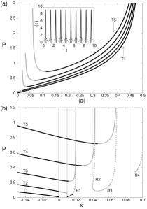
Fig. 2: Solid lines show power of the first five SDSs vs $|q|$ (a) and vs $\kappa$ (b) for $j=-1$. Dashed lines in (b) show $j=+1$ SDSs. The other parameters as in Fig. 1. Black/gray lines mark stable/unstable solutions.

Using the above approach we have been able to find families of spectrally localized solutions, which we called spectral-discrete solitons (SDSs). Examples of SDSs corresponding to the first and second modes of the harmonic oscillator are shown in Figs. 1(a), (b) as functions of the coherence $|q|$. Doing numerical continuation of SDSs along $\kappa$ we computed $q$ at each step and used $|q|$ as a parameter in Figs. 1,2. $|q|$ tends to its maximum, $|q|=1/2$, when $|S|\gg 1$. Notably, the derivative of $|q|$ in $|S|$ tends to zero under the same conditions, i.e. $|q|$ becomes field independent. Thus, perhaps counter-intuitively, in the limit of the maximum Raman coherence Eqs. (1) become quasi-linear. Oppositely, the nonlinearity of our system is at its maximum for $|S|\ll 1$. The dependencies of the power $P=\sum_{n}|E_{n}|^{2}$ of the first five SDSs (labeled as $T1$-$T5$ in all Figs.) as functions of both $|q|$ and $\kappa$ are shown in Figs. 2(a,b). Black lines in Fig. 2 correspond to the stable SDSs and gray ones to the unstable ones. The boundaries of existence in $\kappa$ of some of the SDSs (see vertical lines in Fig. 2(b)) are given by the linear spectrum of Eqs. (1).

$|q|$ tends to $1/2$, when $\kappa$ is negative and its absolute value increases. For these parameter values, the shape of SDSs is very close to the modes of the linear harmonic oscillator. Since nonlinearity is diminished under these conditions, it is not surprising that SDSs are stable for $\kappa<0$. Diffraction in the frequency space increases for large $|q|$, and so is the number of excited Raman harmonics. Thus in the time domain, the quasi-linear SDSs represent a periodic sequence of ultra-short pulses, see the full line in the inset to Fig. 2(a), where the intensities of the total field $I=\left|\sum_{n}E_{n}(z)\exp(i\omega_{n}t)\right|^{2}$ are plotted. Here, $t$ is dimensionless time. At intermediate and low values of Raman coherence, the diffraction in frequency space is relatively small and nonlinear interaction starts to play an important role. Both of the above factors contribute to stronger spectral localization of SDSs, see Fig. 1. The corresponding temporal profiles transform into weakly modulated wavetrains, see the dashed curve in the inset to Fig. 2(a). Dynamical instabilities of the higher order SDSs are readily found in this regime, see Figs. 2(a,b). However, the ground state solution remains stable within the entire range of its existence. An example of evolution of spectral components of the unstable two-peak SDS perturbed by noise is shown in Fig. 3(a). One can see that localization due to potential $\beta(\omega)$ remains unaffected by the instability development. Shape deformation of the unstable SDS increasing its power leads to formation of spectral breathers, see Fig. 3(b). Note that the dependencies of $P$ on $\kappa$ in Fig. 2(a) indicate that transition from the stable to unstable regimes may be driven by the Vakhitov-Kolokolov type of instability [2].

Fig. 3: Propagation of the unstable two-peak SDS with noise added (a) and with its power increased by a regular correction (b). $\kappa=0.005$ and $|q|\approx 0.013$. The other parameters as in Fig. 1.

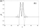
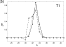
Fig. 4: (a) An example of SDS for $j=+1$. $\kappa=0.01$, $|q|\approx 0.00035$ (black lines and circles), $\kappa=0.02$, $|q|\approx 0.016$ (gray lines and squares). (b) Examples of transformation of a single peak $j=-1$ SDS for non-zero $p_{3}=0.005$ (dashed line, open circles) and non-zero $\alpha=0.008$ (solid gray line, gray squares). Solid black line and filled circles mark the $p_{3}=\alpha=0$ case. $\kappa=-0.004$ for all solutions. The other parameters as for Fig. 1.

The above discussion focuses on the SDSs branches found for negative Raman detuning $j=-1$ ($T$-type SDS), while the dashed lines in Fig. 2(b) mark the solutions existing for $j=+1$ ($R$-type SDS). The latter ones are mostly unstable, because for $j=+1$ the discrete diffraction is not compensated by the normal GVD. However, $R$-type SDSs are still of some interest because they are involved with the bifurcations joining them to the $T$-type SDSs. An example of an $R$-type solution is shown in Fig. 4(a). We have also found that the SDS branches shown in Fig. 2 can be smoothly continued using the Newton method into the region of nonzero higher order dispersions and nonzero values of $\alpha$, which results in the appearance of asymmetries in their profiles, see Fig. 4(b). Interestingly, this creates an opportunity to compensate asymmetries due to unavoidable $p_{3}$ with controllable $\alpha$. A more detailed discussion of the existence and stability of SDSs goes beyond our present scope.

Summary: We reported families of spectral-discrete solitons existing due to the balance between the effective diffraction in frequency space induced by Raman coherence, and the spectral trapping created by the normal GVD. The SDS concept has allowed us to study the problem of short pulse generation using methods of nonlinear dynamics. We demonstrated that spectrally broad, but still localized, solutions associated with trains of short-pulses are typically stable and that solutions strongly localized in frequency space, corresponding to the weakly modulated waves, tend to be dynamically unstable. Our approaches could be useful in the analysis of other nonlinear systems which generate regular frequency combs.

References

- [1] D.N. Christodoulides, F. Lederer, and Y. Silberberg, Nature 424, 817 (2004) and references therein.
- [2] Y.S. Kivshar and G.P. Agrawal, Optical Solitons (Academic, New York, 2003) and references therein.
- [3] A.V. Sokolov and S.E. Harris, J. Opt. B 5, 1 (2003) and references therein.
- [4] S.E. Harris and A.V. Sokolov, Phys. Rev. A 55, R4019 (1997).
- [5] D.D. Yavuz, A.V. Sokolov, and S.E. Harris, Phys. Rev. Lett. 84, 75 (2000).
- [6] S. Flach, M.V. Ivanchenko, and O.I. Kanakov, Phys. Rev. Lett. 95, 064102 (2005).