Gaussian paradox and clustering in intermittent turbulent signals

Abstract

A relation between intermittency and clustering phenomena in velocity field has been revealed for homogeneous fluid turbulence. It is described how the intermittency exponent can be split into sum of two other exponents. One of these exponents (cluster-exponent) characterizes clustering of the ’zero’-crossing points in nearly Gaussian velocity field and another exponent is related to the tails of the velocity probability distribution. The cluster-exponent is uniquely determined by the energy spectrum of the nearly Gaussian velocity field and entire dependence of the intermittency exponent on Reynolds number is determined by the cluster-exponent.

Relation between intermittency of dissipation field fs ,sa ,g and clustering in turbulent velocity field sb1 ; sb2 is still very obscure. Taking into account that turbulent velocity itself is nearly Gaussian my the clustering phenomenon in the velocity field should be also a ’Gaussian’ one, while the intermittency phenomenon is usually associated just with non-Gaussian properties of the velocity derivatives fs ,sa ,my . On the other hand, it is expected that high frequency events in the velocity field should provide significant contribution to the turbulent dissipation and, especially, to its high order moments fs ,sms ,bt .

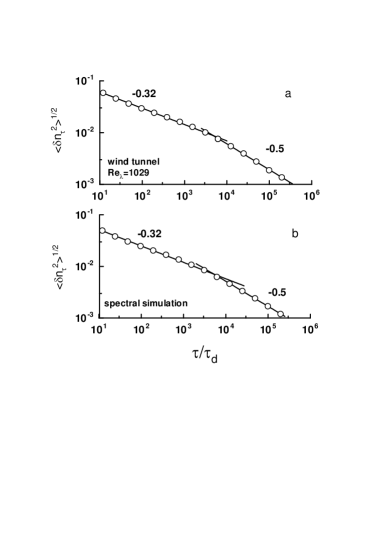
Figure 1: Standard deviation of the running density fluctuations against $\tau$ for for the velocity fluctuations measured in the wind-tunnel pkw (Fig. 1a) and for their Gaussian spectral simulation (Fig. 1b).

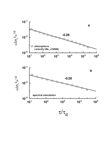
Figure 2: As in Fig. 1 but for atmospheric surface layer at $Re_{\lambda}=19000$ sd (Fig. 2a) and for its Gaussian spectral simulation (Fig. 2b).

Therefore, to find relationship between the two phenomena is rather a non-trivial task that demands special tools. In our recent papers sb1 ,sb2 we introduced a cluster-exponent to describe quantitatively clustering in turbulent velocity field and we found an empirical relationship between the cluster- and intermittency exponents. In present paper we will describe how the intermittency exponent can be split into sum of two other exponents (Eq. 6). One of these exponents is the cluster-exponent sb1 and another exponent is related to the tails of the velocity probability distribution. We also will show that the cluster-exponent is uniquely determined by the energy spectrum of the nearly Gaussian velocity field. This simple splitting of the intermittency exponent on the Gaussian and ’tail’ components can be considered as a solution of the problem which was formulated above. Moreover, for finite Reynolds numbers $Re_{\lambda}$ the energy spectrum depends on $Re_{\lambda}$ and, therefore, the cluster-exponents depends on $Re_{\lambda}$, while the ’tail’ component of the intermittency exponent is independent on $Re_{\lambda}$. Therefore, the entire dependence of the intermittency exponent on $Re_{\lambda}$ is uniquely determined by its Gaussian component (through the clustering phenomenon) that we will call Gaussian paradox.

Let us count the number of ’zero’-crossing points of the signal in a time interval $\tau$ and consider their running density $n_{\tau}$. Let us denote fluctuations of the running density as $\delta n_{\tau}=n_{\tau}-\langle n_{\tau}\rangle$, where the brackets mean the average over long times. We will be interested in the scaling variation of the standard deviation of the running density fluctuations $\langle\delta n_{\tau}^{2}\rangle^{1/2}$ with $\tau$

$$\langle\delta n_{\tau}^{2}\rangle^{1/2}\sim\tau^{-\alpha_{n}}$$

For white noise it can be derived analytically molchan ,lg that $\alpha_{n}=1/2$ (see also sb1 ). In Figure 1a and 2a we show calculations of the standard deviation for a turbulent velocity signal obtained in the wind-tunnel experiment pkw and for a velocity signal obtained in an atmospheric experiment sd respectively. The straight lines are drawn in the figures to indicate scaling (1). One can see two scaling intervals in Fig. 1. The left scaling interval covers both dissipative and inertial ranges, while the right scaling interval covers scales larger then the integral scale of the flow. While the right scaling interval is rather trivial (with $\alpha_{n}=1/2$, i.e. without clustering), the scaling in the left interval (with $\alpha_{n}<1/2$) indicates clustering of the high frequency fluctuations. The cluster-exponent $\alpha_{n}$ decreases with increase of $Re_{\lambda}$, that means increasing of the clustering (as it was expected from qualitative observations).

To describe intermittency a running average of fluctuations of the dissipation rate $\varepsilon(t)$ of the velocity signal $u(t)$ can be used po (see also a discussion in lp )

$$\langle\delta\varepsilon_{\tau}^{2}\rangle^{1/2}\sim\tau^{-\alpha_{\varepsilon}}$$

where

$$\varepsilon_{\tau}=\frac{\int_{0}^{\tau}\varepsilon(t)dt}{\tau}$$

and $\langle\delta\varepsilon_{\tau}^{2}\rangle^{1/2}$ is standard deviation of $\varepsilon_{\tau}$. Figure 3 shows an example of the scaling (2) providing the intermittency exponent $\alpha_{\varepsilon}$ for the wind-tunnel data (see po for more details and Fig. 5 for the statistical errors).

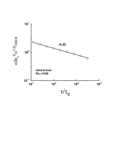
Figure 3: Intermittency exponent as slope of the straight line for the longitudinal velocity signal obtained in the wind tunnel experiment pkw at $Re_{\lambda}=1029$.

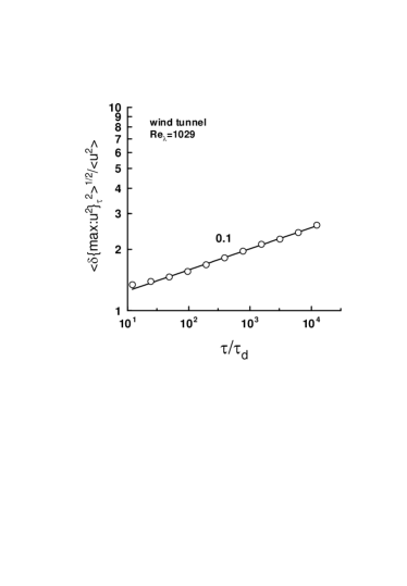
Figure 4: Statistical (’tail’) exponent $\alpha_{m}\simeq 0.1$ as slope of the straight line for the longitudinal velocity signal obtained in the wind tunnel experiment pkw at $Re_{\lambda}=1029$.

Events with high concentration of the zero-crossing points in the intermittent turbulent velocity signal provide main contribution to the $\langle\delta\varepsilon_{\tau}^{2}\rangle$ due to high concentration of the statistically significant local maximums in these events bt . Therefore, one can make use of statistical version of the theorem ’about mean’ in order to estimate the standard deviation

$$\langle\delta\varepsilon_{\tau}^{2}\rangle^{1/2}\sim\langle\delta\{\max:u^{2}\}_{\tau}^{2}\rangle^{1/2}\langle\delta n_{\tau}^{2}\rangle^{1/2}$$

where $\{\max:u^{2}\}_{\tau}$ is maximum of $u(t)^{2}$ in the interval of length $\tau$. Value of $\langle\delta\{\max:u^{2}\}_{\tau}^{2}\rangle^{1/2}$ should grow with $Re_{\lambda}$ (due to increasing of $\langle u^{2}\rangle$) and, statistically, with the length of interval $\tau$ (the later growth is expected to be self-similar), i.e.

$$\langle\delta\{\max:u^{2}\}_{\tau}^{2}\rangle^{1/2}=C(Re_{\lambda})\cdot\tau^{\alpha_{m}}$$

where constant $C(Re_{\lambda})$ is a monotonically increasing function of $Re_{\lambda}$, and the statistical (’tail’) exponent $\alpha_{m}\geq 0$ is independent on $Re_{\lambda}$. Fig. 4 shows an example of scaling (5) providing the statistical (’tail’) exponent $\alpha_{m}\simeq 0.10\pm 0.01$. Substituting (5) into (4) and taking into account (1) and (2) we can infer a relation between the scaling exponents

$$\alpha_{\varepsilon}=\alpha_{n}-\alpha_{m}$$

Unlike the exponent $\alpha_{m}$ the exponent $\alpha_{n}$ depends on $Re_{\lambda}$ (see Fig. 2 and Ref. sb1 ). Therefore, we can learn from (6) that just the clustering of the high frequency velocity fluctuations ($\alpha_{n}$ in (6)) is responsible for dependence of the intermittency exponent $\alpha_{\varepsilon}$ on the $Re_{\lambda}$.

It is naturally consider the exponent functions through $\ln R_{\lambda}$: $\alpha=\alpha(\ln Re_{\lambda})$ sb1 ,cgh ,bg (see also Appendix). Following to the general idea of Ref. bg (see also sb1 ) let us expend this function for large $Re_{\lambda}$ in a power series:

$$\alpha(\ln Re_{\lambda})=\alpha(\infty)+\frac{a_{1}}{\ln Re_{\lambda}}+\frac{a_{2}}{(\ln Re_{\lambda})^{2}}+...$$

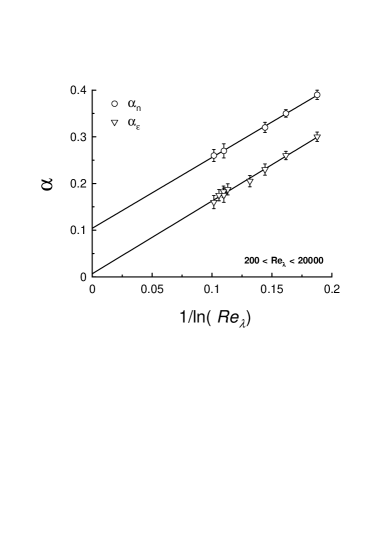
Figure 5: The cluster-exponent: $\alpha_{n}$ (circles), against $1/\ln Re_{\lambda}$ for velocity signal at different values of Reynolds number ($200<Re_{\lambda}<20000$). Scaling exponent $\alpha_{\varepsilon}$ (triangles) for fluctuations of the dissipation rate of the velocity signals.

In Figure 5 we show the values of $\alpha_{n}$ (circles) and $\alpha_{\varepsilon}$ (triangles) calculated for the velocity signals against $1/\ln Re_{\lambda}$ for $200<Re_{\lambda}<20000$ (the data are taken from the wind-tunnel experiment pkw , from the atmospheric experiment sd , from a mixing layer and an atmospheric surface experiments po ). The straight lines (the best fit) indicate approximation with the two first terms of the power series expansion (7)

$$\alpha_{n}(\ln Re_{\lambda})\simeq 0.1+\frac{3/2}{\ln Re_{\lambda}},~{}~{}~{}~{}~{}~{}~{}~{}\alpha_{\varepsilon}(\ln Re_{\lambda})\simeq\frac{3/2}{\ln Re_{\lambda}}$$

This means, in particular, that

$$\lim_{Re_{\lambda}\rightarrow\infty}\alpha_{n}\simeq 0.1,~{}~{}~{}~{}~{}\lim_{Re_{\lambda}\rightarrow\infty}\alpha_{\varepsilon}\simeq 0$$

The closeness of the constants $a_{1}\simeq 3/2$ (the slopes of the straight lines in Fig. 5) in the approximations (8) of the cluster-exponent $\alpha_{n}$ and of the intermittency exponent $\alpha_{\varepsilon}$ confirms the relationship (6) with $\alpha_{m}\simeq 0.1$ (cf Figs. 4 and 5).

Thus one can see that entire dependence of the intermittency exponent $\alpha_{\varepsilon}$ on $Re_{\lambda}$ is uniquely determined by dependence of the cluster-exponent $\alpha_{n}$ on $Re_{\lambda}$. On the other hand, the cluster-exponent $\alpha_{n}$ itself is uniquely determined by energy spectrum of the velocity signal at suggestion that the velocity field is nearly Gaussian. This means that energy spectrum uniquely determines dependence of the intermittency exponent on the Reynolds number $Re_{\lambda}$. From conventional point of view on intermittency it seems as a paradox.

We use spectral simulation to illustrate the uniquely relationship between energy spectrum and cluster-exponent for the Gaussian signals; i.e. we generate Gaussian stochastic signal with energy spectrum given as data (the spectral data is taken from the original velocity signals). Obviously, the pure Gaussian signal obtained in such simulation does not possesses the turbulent intermittency properties resulting in the estimate (4). Figures 1b and 2b show, as examples, results of such simulation for the wind-tunnel velocity data (Fig. 1b) and for the atmospheric surface layer (Fig. 2b). Namely, Figures 1a and 2a show results of the calculations for the original velocity signals and Figs. 1b, and 2b show corresponding results obtained for the spectral simulations of the signals (to be sure, for the both Gaussian simulations $\alpha_{\varepsilon}\simeq 0.5$ unlike of $\alpha_{n}$).

It is interesting to note that for isotropic turbulence with prominent inertial (Kolmogorov) range the only small-scale edge of the inertial range (this scale depends on $Re_{\lambda}$) determines value of the cluster-exponent $\alpha_{n}$ corresponding to the spectrum. I.e. role of the viscous dissipation in this respect is reduced to the effective small-scale ’cut-off’ effect and just dependence of the ’cut-off’ scale on $Re_{\lambda}$ determines dependence of the intermittency exponent $\alpha_{\varepsilon}$ on $Re_{\lambda}$ through equation (6) for such flows.

I thank K.R. Sreenivasan for inspiring cooperation. I also thank G. Falkovich, C.H. Gibson, A. Praskovsky, and V. Steinberg for discussions.

I Appendix

Thin vortex tubes (or filaments) are the most prominent hydrodynamical elements of turbulent flows batchelor . The filaments are unstable in 3-dimensional space. In our recent paper sb1 we investigated this instability in order to renormalize the Taylor microscale Reynolds number.

A straight line-vortex can readily develop a kink propagating along the filament with a constant speed. To estimate the velocity of propagation of such a kink let us first recall the properties of a ring vortex batchelor . Its speed $v$ is related to its diameter $\lambda$ and strength $\Gamma$ through

$$v=\frac{\Gamma}{2\pi\lambda}\ln\left(\frac{\lambda}{2\eta}\right),$$

where $\eta$ is the radius of the core of the ring and $\lambda/2\eta\gg 1$ (see figure 6).

If, for instance, a straight line-vortex develops a kink with a radius of curvature $\lambda/2$, then self-induction generates a velocity perpendicular to the plane of the kink. This velocity can be also calculated using (A.1).

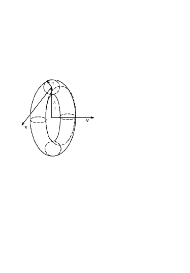
Figure 6: The vortex ring and its velocity.

One can guess that in a turbulent environment, the most unstable mode of a vortex tube with a thin core of length $L$ (integral scale) and radius $\eta$ (Kolmogorov or viscous scale), will be of the order $\lambda$: Taylor-microscale my ,saf . Then, the characteristic scale of velocity of the mode with the space scale $\lambda$ can be estimated with help of equation (A.1). Noting that the Taylor-microscale Reynolds number is defined as my

$$Re_{\lambda}=\frac{v_{0}\lambda}{\nu},$$

where $v_{0}$ is the root-mean-square value of a component of velocity. It is clear that the velocity that is more relevant (at least for the processes related to the vortex instabilities) for the space scale $\lambda$ is not $v_{0}$ but $v$ given by (A.1). Therefore, corresponding effective Reynolds number should be obtained by the renormalization of the characteristic velocity in (A.2), as

$$Re_{\lambda}^{eff}=\frac{v\lambda}{\nu}\sim\frac{\Gamma}{2\pi\nu}\ln\left(\frac{\lambda}{2\eta}\right).$$

It can be readily shown from the definition that

$$\frac{\lambda}{\eta}=const~{}Re_{\lambda}^{1/2}$$

where $const=15^{1/4}\simeq 2$. Hence

$$Re_{\lambda}^{eff}\sim\frac{\Gamma}{4\pi\nu}\ln(Re_{\lambda})$$

The strength $\Gamma$ can be estimated as

$$\Gamma\sim 2\pi v_{\eta}\eta$$

where $v_{\eta}=\nu/\eta$ is the velocity scale for the Kolmogorov (or viscous) space scale $\eta$ my . Substituting (A.6) into (A.5) we obtain

$$Re_{\lambda}^{eff}\sim\ln(Re_{\lambda}).$$

Thus, for turbulence processes determined by the vortex instabilities the relevant dimensionless characteristic is $\ln(Re_{\lambda})$ rather than $Re_{\lambda}$ (cf Eq. (7) and Fig. 5).

References

- (1) G. Falkovich and K.R. Sreenivasan, Physics Today, 59, 43 (2006).
- (2) K.R. Sreenivasan and R.A. Antonia, Annu. Rev. Fluid Mech., 29, 435 (1997).
- (3) C.H. Gibson, Proc. Roy. Soc. London, Ser. A, 434, 149 (1991).
- (4) K.R. Sreenivasan and A. Bershadskii, J. Fluid Mech., 54 477 (2006).
- (5) K.R. Sreenivasan and A. Bershadskii, J. Stat. Phys., in press (2006).
- (6) Monin A. S. and Yaglom A.M., 1975 Statistical Fluid Mechanics: Mechanics of Turbulence, V. 2 (The MIT Press, Cambridge).
- (7) G. Stolovitzky, C. Meneveau and K.R. Sreenivasan, Phys. Rev. Lett., 80, 3883 (1998).
- (8) A. Bershadskii and A. Tsinober, Phys. Lett. A, 165 37-41 (1992).
- (9) G. Molchan, private communication.
- (10) M.R. Leadbetter and J.D. Gryer, Bull. Amer. Math. Soc. 71, 561 (1965).
- (11) B.R. Pearson, P.-A. Krogstad and W. van de Water, Phys. Fluids, 14, 1288 (2002).
- (12) K.R. Sreenivasan and B. Dhruva, Prog. Theor. Phys. Supp., 130 103 (1998).
- (13) A. Praskovsky and S. Oncley, Fluid. Dyn. Res., 21, 331 (1997).
- (14) V.S. L’vov and I. Procaccia, Phys. Rev. Lett., 74, 2690 (1995).
- (15) B. Castaing, Y. Gagne and E.J. Hopfinger, Physica D, 46, 177 (1990).
- (16) G.I. Barenblatt and N. Goldenfeld, Phys. Fluids, 7, 3078 (1995).
- (17) G.K. Batchelor, An Introduction to Fluid Dynamics (Cambridge University Press, Cambridge, 1970).
- (18) P.G. Saffman, Lectures on Homogeneous Turbulence. In Topics in Nonlinear Physics (ed. N.J. Zabusky), pp. 485-614, Springer-Verlag, New York, 1968.