Many-body perturbation calculation of spherical nuclei with a separable monopole interaction: I. Finite Nuclei

Abstract

We present calculations of ground state properties of spherical, doubly closed-shell nuclei from ¹⁶O to ²⁰⁸Pb employing the techniques of many-body perturbation theory using a separable density dependent monopole interaction. The model gives results in Hartree-Fock order which are of similar quality to other effective density-dependent interactions. In addition, second and third order perturbation corrections to the binding energy are calculated and are found to contribute small, but non-negligible corrections beyond the mean-field result. The perturbation series converges quickly, suggesting that this method may be used to calculate fully correlated wavefunctions with only second or third order perturbation theory. We discuss the quality of the results and suggest possible methods of improvement.

I Introduction

The central problem of nuclear structure theory is the solution of the many-body Schrödinger equation (MBSE). For Hamiltionans of interest in the nuclear case, an analytic solution is impossible, and one is compelled to use some approximation, either in the numerical solution of the equation or the specification of the Hamiltonian, or both.

Approaching the problem with the aim of using as realistic a representation of the potential as possible usually means fitting a combination of a meson exchange and phenomenological interaction to low-energy nucleon-nucleon scattering data and properties of few-body systems. To get good agreement with experiment both two- and three-body forces seem to be necessary. Recent examples of such potentials include the Bonn [1], the Argonne two-body [2] with Urbanna 3-body[3], Nijmegen [4] and Moscow [5] potentials, the last of which also incorporates quark degrees of freedom. These forces share the property of having a hard repulsive core which is a natural consequence of meson-exchange. It is this hard core which presents the difficulty in solving the MBSE. For instance, Hartree-Fock (HF) mean-field calculations with such interactions result in unbound nuclei. Treating corrections beyond the HF approximation order-by-order in perturbation theory is also unsuccessful since the interactions used are non-perturbative. One has to solve the full MBSE numerically in as exact a way as possible using techniques such as Variational Monte-Carlo[6], Green’s Function Monte Carlo[7], the coupled-cluster method[8, 9], and the Fermion Hyper-netted chain model[10]. Using effective interactions derived from realistic potentials, no-core shell-model calculations have been made in light nuclei[11] and heavier nuclei close to closed shells have been treated[13].

The computational difficulty of performing numerically exact solutions of the MBSE has limited the techniques to light nuclei, for instance $A=8$ results have been published recently using the Argonne $v18$ and Urbanna IX potentials in the GFMC framework[12]. In this work, it is seen that although the lightest nuclei are reproduced very well, the quantitative comparison of theory to data gets worse as $A$ increases. This may be due to the necessarily phenomenological nature of the three–body potential, a problem which may be overcome with re-fitting. On the other hand, it is not obvious that higher-body forces will not prove necessary or that the concept of a bare interaction between nucleons is valid for small distances.

Attempts were made in the late sixties primarily by the Kerman group at MIT to parameterize the NN interaction in such a way that it is weak in the sense of being perturbative. Such a weak interaction allows one to perform Hartree-Fock calculations to obtain a reasonable approximation to the full wavefunction and then to calculate corrections in perturbation theory. While this technique seems very attractive, the result obtained were only moderately successful at reproducing experimental data[14, 15, 16, 17, 18], a fact which was presumed to be due to inadequacies in the potentials used. The efficacy of developing a suitable interaction when similar, though more complicated, techniques were available for realistic interactions has been questioned[19] and no better interaction was developed. Separable parameterizations, particularly the quadrupole-quadrupole interaction[20, 21], have retained currency, as residual interactions [41]. Even when the interactions are too strong for regular perturbation theory, separable interactions requiring solution of Brückner Hartree-Fock equations have proved fruitful[22] because of their simplicity.

On the other hand, interactions have been developed which are not intended for use in the full MBSE, but rather to give good results with a Hartree-Fock calculation alone. Good quantitative success came with the zero-range density-dependent force of Ehlers and Moszkowski[24] and Skyrme’s interaction[23], used in HF calculations by Vautherin and Brink [25] and subsequently by many others, and also Gogny’s finite-range interaction[26]. Skyrme’s interaction has been particularly successful, in part due to its simple form, that of a delta function, which leads to easy calculation, even of the exchange part of the force. This computational simplicity has allowed extensive study of the properties of nuclei to be made with the Skyrme interaction across the entire range of nuclei in the periodic table [27, 48, 50]. Related somewhat to the Skyrme-Hartree-Fock model is the Relativistic Mean Field (RMF) approach[28, 29], which also gives single-particle motion in a mean field, but as a solution to the Dirac equation as opposed to the Schrödinger equation. The RMF approach has some nice features such as the natural occurrence of the spin-orbit splitting without recourse to an assumed spin-orbit interaction.

These mean-field models are inherently single-particle in nature. The forces used are not intended to be used in the MBSE, nor are explicit corrections beyond the mean-field part of the framework, although Skyrme’s interaction can be considered as a phenomenological G-matrix equivalent[30], and in that sense includes a subset of possible correlation effects in the mean-field. Although appropriate for use in mean-field calculations, Skyrme’s interaction would actually diverge in perturbation theory because of the zero range. This compels one to use a different interaction to obtain correlation beyond the mean field than was used to create it. Extra residual forces are used, such as pairing[32], or shell model interactions[31] to allow for more general wavefunctions and obtain more accurate reproduction of the physics, or certain approximations are used such as RPA[33], which can describe certain observables, particularly those of giant resonance states and other forms of collective motion, but not others. It is thought that correlations should be particularly important in nuclei at the limits of stability, where the nucleons nearest the Fermi level couple strongly to the continuum.

We revisit the idea that it is possible to parameterize a nuclear interaction in such a way that it is weak enough with which to perform perturbation theory, thereby allowing correlated wavefunctions and observables to be calculated across the entire range of nuclei. Using the separable ansatz of previous “weak” interactions we have developed a density dependent interaction which we hope will provide some insight into the correlation structure of nuclear wavefunctions while retaining the quantitative power of contemporary effective interactions used in Hartree-Fock. In contrast to previous work, the interaction is designed to be an effective interaction with parameters fitted to the properties of finite nuclei within the calculation framework for which it is intended.

The paper is organized as follows. In Section 2 we briefly review basics of many-body perturbation theory. The separable interaction, used in the present work is given and discussed in Section 3. Results of the calculation for doubly magic nuclei are summarized in Section 4. Derivation of the HF energy and potential is outlined in Appendix A.

II Single particle models and many-body perturbation theory

For standard perturbation theory to be successful, the Hamiltonian must be separated into two parts, one which is solvable ($H_{0}$), and another which is “small” ($H_{1}$). The Hamiltonian for a many-fermion problem in which the particles interact via one- and two-body interactions may be written schematically as

$$H=\sum_{ij}\langle i|U|j\rangle\,a^{\dagger}_{i}a_{j}+\frac{1}{4}\sum_{ijkl}\langle ij|V|kl\rangle a^{\dagger}_{i}a^{\dagger}_{j}a_{l}a_{k}.$$ (1)

Typically, the one-body part of the Hamiltonian is just the kinetic energy. This is a unsuitable choice for $H_{0}$ in the case of nuclei since the eigenstates of this operator, namely plane wave states, are not close enough to the exact eigenstates of the full Hamiltonian and $H_{1}$ is thus not small. By adding and subtracting a one-body term, $U^{\prime}$, of ones choice, the $H_{0}$ part of the Hamiltonian may be solvable to give a wavefunction close to the solution of the full problem, thereby making the corrections from the $H_{1}$ part small enough for perturbation theory to succeed. Schematically the Hamiltonian is now split up into two terms;

$$H=\underbrace{\sum_{ij}\langle i|U+U^{\prime}|j\rangle\,a^{\dagger}_{i}a_{j}}_{H_{0}}+\underbrace{\frac{1}{4}\sum_{ijkl}\langle ij|V|kl\rangle a^{\dagger}_{i}a^{\dagger}_{j}a_{l}a_{k}-\sum_{ij}\langle i|U^{\prime}|j\rangle\,a^{\dagger}_{i}a_{j}}_{H_{1}}.$$ (2)

One practical choice of $U^{\prime}$ is a simple, analytically-solvable external potential, typically – in the nuclear case – of harmonic oscillator or Woods-Saxon form. In such a case, all of the physics of the nuclear interaction is in the residual part, $H_{1}$. Unfortunately, for sensible choices of two-body interaction, the residual part of the Hamiltonian is non-perturbative in the basis obtained from the solution of the one-body part of the Hamiltonian, and one has to perform more exact and exacting interaction shell-model calculations to arrive at a meaningful result. Traditionally, this has involved the diagonalisation of large matrices, or more recently, auxiliary field Monte-Carlo calculations in the SMMC[34].

Another popular choice for $U^{\prime}$ is that of the Hartree-Fock mean-field. The HF mean-field potential is usually derived from the full Hamiltonian by a variational principle. Viewed in this way, it is the one-body potential whose occupied eigenstates form the lowest energy Slater-Determinant many-body wavefunction possible for the full many-body Hamiltonian. Using such a one-body potential, some physics of the two-body interaction is included in the single-particle problem. With a judicious choice of interaction, one ought to be able to produce very good results, since the approximation of the nucleus as a system of non-interacting particles in a mean-field is known to be a good one. Using the HF potential for $U^{\prime}$ has the added attraction that it leads to vanishing first order corrections to the energy in perturbation theory. In this case, using Wick’s theorem[35], one can re-write (1) as

$$H=\underbrace{E_{0}+\sum_{i<\epsilon_{F}}\varepsilon_{i}:\!a^{\dagger}_{i}a_{i}\!:}_{H_{0}}+\underbrace{\frac{1}{4}\sum_{ijkl}\langle ij|V|kl\rangle:\!a^{\dagger}_{i}a^{\dagger}_{j}a_{l}a_{k}\!:}_{H_{1}}$$ (3)

where $H_{0}$ is the HF mean-field Hamiltonian and $H_{1}$ is the perturbing Hamiltonian. Note that $H_{1}$ is just the full two-body interaction matrix elements with a time-ordered product of creation and annihilation operators. The perturbation series for the energy is ordered by the number of matrix elements of the potential. Usually a diagrammatic representation is used[36]. One can write down the number of diagrams for any particular order of perturbation theory. We have evaluated these for the vacuum amplitude up to order seven. The results are presented in Table I. One sees that, for the method of direct evaluation of diagrams by order to be effective, the series must be sufficiently converged by fourth, or perhaps fifth, order.

In this work, the second and third order diagrams for the vacuum amplitude, as shown in Figs. 1 and 2, are calculated. Their algebraic form is given here as

$$E_{2} = \frac{1}{4}\sum\limits_{ab<\epsilon_{F}}\sum\limits_{rs>\epsilon_{F}}\frac{|\langle ab|\tilde{V}|rs\rangle|^{2}}{\epsilon_{a}+\epsilon_{b}-\epsilon_{r}-\epsilon_{s}}$$ (4)

$$E_{3}^{(pp)} = \frac{1}{8}\sum\limits_{ab<\epsilon_{F}}\sum\limits_{rs>\epsilon_{F}}\sum\limits_{tu>\epsilon_{F}}\frac{\langle ab|\tilde{V}|rs\rangle\langle rs|\tilde{V}|tu\rangle\langle tu|\tilde{V}|ab\rangle}{(\epsilon_{a}+\epsilon_{b}-\epsilon_{r}-\epsilon_{s})(\epsilon_{a}+\epsilon_{b}-\epsilon_{t}-\epsilon_{u})}$$ (5)

$$E_{3}^{(hh)} = \frac{1}{8}\sum\limits_{ab<\epsilon_{F}}\sum\limits_{cd<\epsilon_{F}}\sum\limits_{rs>\epsilon_{F}}\frac{\langle ab|\tilde{V}|rs\rangle\langle cd|\tilde{V}|ab\rangle\langle rs|\tilde{V}|cd\rangle}{(\epsilon_{a}+\epsilon_{b}-\epsilon_{r}-\epsilon_{s})(\epsilon_{c}+\epsilon_{d}-\epsilon_{t}-\epsilon_{u})}$$ (6)

$$E_{3}^{(ph)} = \sum\limits_{abc<\epsilon_{F}}\sum\limits_{rst>\epsilon_{F}}\frac{\langle ab|\tilde{V}|rs\rangle\langle cr|\tilde{V}|at\rangle\langle st|\tilde{V}|cb\rangle}{(\epsilon_{a}+\epsilon_{b}-\epsilon_{r}-\epsilon_{s})(\epsilon_{b}+\epsilon_{c}-\epsilon_{s}-\epsilon_{t})}$$ (7)

in which the tildes over the potential indicate the matrix element is antisymmetrized. The state vectors label HF single-particle states, whose energies are given by the subscripted $\epsilon$.

It is important to note that our interaction is not intended to fit scattering data, having, as it does, density dependence. On the level of the perturbation theory it is necessary to treat the density functions as just the spatial form of the interaction, rather than a representation of a many-body force. This is to be considered a part of the present model. To do otherwise would be to surrender the simplifications our weak, separable potential affords.

In the present work, the Hartree-Fock problem is solved in a basis of spherical harmonic oscillator states. This yields, along with the hole states, a large number of particle states, with which to directly evaluate the sums of the perturbation series. A sufficient number of states is used so that the particle states are oscillatory over the size of the nucleus and that both the HF solution and the perturbation corrections are reasonably converged.

III Interaction

We have developed an interaction written in the form of a sum of separable terms, which is to say it is in the form $V(r_{1},r_{2})\sim\sum g(r_{1})g(r_{2})$. The functions $g$ carry no angular momentum ($l=0$), and the force is dubbed a monopole-monopole interaction. For future applications, it is in intended to include higher multipole forces, with $l=1,2,\ldots$, within our framework as these will presumably be necessary for calculation of excited states and deformed nuclei. Although higher multipole forces will contribute to spherical nuclei from the exchange term in Hartree Fock order and via correlations in perturbation theory, they are not included in the present calculation since it seems unwise to attempt to fit the parameters of such forces to spherical nuclei alone.

In coordinate space, the monopole interaction is written as

$$V(\vec{r}_{1},\vec{r}_{2}) = W_{a}f_{a}\rho^{\beta_{a}}(\vec{r}_{1})\rho^{\beta_{a}}(\vec{r}_{2})(1+a_{a}(\tau_{1}^{+}\tau_{2}^{-}+\tau_{1}^{-}\tau_{2}^{+})+b_{a}t_{1z}t_{2z})$$ (8)

$$+ W_{r}f_{r}\rho^{\beta_{r}}(\vec{r}_{1})\rho^{\beta_{r}}(\vec{r}_{2})(1+a_{r}(\tau_{1}^{+}\tau_{2}^{-}+\tau_{1}^{-}\tau_{2}^{+})+b_{r}t_{1z}t_{2z})$$ (9)

$$+ k\nabla_{\!\!1}^{2}\rho(\vec{r}_{1})\nabla_{\!\!2}^{2}\rho(\vec{r}_{2}),$$ (10)

where the function $f_{\xi}$ is defined as

$$f_{\xi}=\left[\int{\rm d}^{3}\vec{r}\,\rho^{\alpha_{\xi}}(\vec{r})\right]^{-1},$$ (11)

for subscripts $\xi=a$ and $\xi=r$. Throughout this work, the three terms in (10) are referred to, in the order they appear in the above expression, as the attractive, repulsive and derivative terms.

In addition, the spin-orbit force is taken to be

$$V_{\rm s-o}(r)=c\frac{1}{r}\frac{\partial\rho}{\partial r}\vec{l}\cdot\vec{s},$$ (12)

which is similar to that used in the modified delta interaction [24].

The parameters $W_{a}$, $\alpha_{a}$, $\beta_{a}$, $a_{a}$, $b_{a}$, $W_{r}$, $\alpha_{r}$, $\beta_{r}$, $a_{r}$, $b_{r}$, $k$ and $c$ are to be fitted to experimental data.

One notices that the two-body interaction consists of a sum of terms, each of which is separable in form and that the expressions for the attractive and repulsive terms in (10) differ only by the values of their parameters

The energy, $E_{\rm pot}$, due to the interaction (10) in the Hartree-Fock approximation is derived in Appendix A (A4), (A10), (A41) and is presented here;

$$E_{HF} = T+E_{\rm coul}+E_{\rm pot}=T+E_{\rm coul}+\sum_{\xi=a,r}\Big{\{}\frac{1}{2}W_{\xi}f_{\xi}N_{\xi}^{2}-\frac{1}{2}W_{\xi}f_{\xi}M_{\xi}+\frac{1}{2}W_{\xi}b_{\xi}f_{\xi}(\Delta N_{\xi})^{2}$$ (14)

$$-\frac{1}{2}W_{\xi}f_{\xi}[b_{\xi}M_{\xi}+a_{\xi}M_{\xi}^{(\tau\bar{\tau})}]\Big{\}}+\frac{1}{2}kN_{d}^{2}+cN_{w}$$

where $T$ is the kinetic energy, $E_{\rm coul}$ is the direct Coulomb energy plus exchange in the Slater approximation. The following quantities have been defined;

$$N_{\xi} = \int{\rm d}^{3}\vec{r}\,\rho^{\beta_{\xi}+1}(\vec{r})$$ (15)

$$M_{\xi} = \int\!\int{\rm d}^{3}\vec{r}_{1}{\rm d}^{3}\vec{r}_{2}\,\left[\rho_{p}(\vec{r}_{1},\vec{r}_{2})\rho^{\beta_{\xi}}(\vec{r}_{1})\rho^{\beta_{\xi}}(\vec{r}_{2})\rho_{p}(\vec{r}_{1},\vec{r}_{2})+\rho_{n}(\vec{r}_{1},\vec{r}_{2})\rho^{\beta_{\xi}}(\vec{r}_{1})\rho^{\beta_{\xi}}(\vec{r}_{2})\rho_{n}(\vec{r}_{1},\vec{r}_{2})\right]$$ (16)

$$\Delta N_{\xi} = \int{\rm d}^{3}\vec{r}\,\rho^{\beta_{\xi}}(\vec{r})\left[\rho_{p}(\vec{r})-\rho_{n}(\vec{r})\right]$$ (17)

$$M_{\xi}^{(\tau\bar{\tau})} = \int\!\int{\rm d}^{3}\vec{r}_{1}{\rm d}^{3}\vec{r}_{2}\,\left[\rho_{p}(\vec{r}_{1},\vec{r}_{2})\rho^{\beta_{\xi}}(\vec{r}_{1})\rho^{\beta_{\xi}}(\vec{r}_{2})\rho_{n}(\vec{r}_{1},\vec{r}_{2})+\rho_{n}(\vec{r}_{1},\vec{r}_{2})\rho^{\beta_{\xi}}(\vec{r}_{1})\rho^{\beta_{\xi}}(\vec{r}_{2})\rho_{p}(\vec{r}_{1},\vec{r}_{2})\right]$$ (18)

$$N_{d} = \int{\rm d}^{3}\vec{r}\,\rho(\vec{r})\nabla^{2}\rho(\vec{r})$$ (19)

$$N_{w} = \int{\rm d}^{3}\vec{r}\,\frac{1}{r}\frac{\partial\rho}{\partial r}\rho_{w}(\vec{r})$$ (20)

and the following densities are used:

$$\rho(\vec{r}) = \rho_{p}(\vec{r})+\rho_{n}(\vec{r})=\sum_{i<\epsilon_{F}\in p}\varphi_{i}^{*}(\vec{r})\varphi_{i}(\vec{r})+\sum_{i<\epsilon_{F}\in n}\varphi_{i}^{*}(\vec{r})\varphi_{i}(\vec{r})$$ (21)

$$\rho(\vec{r}_{1},\vec{r}_{2}) = \rho_{p}(\vec{r}_{1},\vec{r}_{2})+\rho_{n}(\vec{r}_{1},\vec{r}_{2})=\sum_{i<\epsilon_{F}\in p}\varphi_{i}^{*}(\vec{r}_{1})\varphi_{i}(\vec{r}_{2})+\sum_{i<\epsilon_{F}\in n}\varphi_{i}^{*}(\vec{r}_{1})\varphi_{i}(\vec{r}_{2})$$ (22)

$$\rho_{w}(\vec{r}) = \sum_{i<\epsilon_{F}}\frac{1}{2}\left(j_{i}(j_{i}+1)-l_{i}(l_{i}+1)-3/4\right)\varphi^{*}_{i}(\vec{r})\varphi_{i}(\vec{r}).$$ (23)

The variation of the total energy is carried out in Appendix A (see A28, A31, A38, A45) . The resulting local Hartree-Fock potential is

$$U_{L,\tau}(x) = \sum_{\xi=a,r}\Big{\{}W_{\xi}f_{\xi}\left[N_{\xi}(\beta_{\xi}+1)+b_{\xi}\Delta_{\tau}N_{\xi}\right]\rho^{\beta_{\xi}}(x)$$ (24)

$$- W_{\xi}(\alpha_{\xi}/2)f_{\xi}^{2}\left[N_{\xi}^{2}+b_{\xi}(\Delta N_{\xi})^{2}-(1+b_{\xi})M_{\xi}-a_{\xi}M_{\xi}^{(\tau\bar{\tau})}\right]\rho^{\alpha_{\xi}-1}(x)$$ (25)

$$- W_{\xi}f_{\xi}\beta_{\xi}\left[(1+b_{\xi})G_{\xi}(x)+a_{\xi}G_{\xi}^{(\tau\bar{\tau})}(x)\right]\rho^{\beta_{x}-1}(x)$$ (26)

$$+ \left[W_{\xi}b_{\xi}\beta_{\xi}f_{\xi}\Delta N_{\xi}\right]\rho^{\beta_{x}-1}(x)\delta\rho(x)\Big{\}}$$ (27)

$$+ 2kN_{d}\nabla^{2}\rho(x)$$ (28)

which differs for protons ($\tau=p$) and neutrons ($\tau=n$) through the function

$$\Delta_{\tau}N_{\xi}=\left\{\begin{array}[]{cl}\Delta N_{\xi},&\tau=p\\ -\Delta N_{\xi},&\tau=n.\end{array}\right.$$ (29)

The other newly-introduced functions in (28) are

$$G_{\xi}(x) = G_{\xi}^{(pp)}(x)+G_{\xi}^{(nn)}(x)=\int\!{\rm d}^{3}\vec{r}\left[\rho_{p}(\vec{r},\vec{x})\rho^{\beta_{\xi}}(r)\rho_{p}(\vec{x},\vec{r})+\rho_{n}(\vec{r},\vec{x})\rho^{\beta_{\xi}}(\vec{r})\rho_{n}(\vec{x},\vec{r})\right]$$ (30)

$$G^{(\tau\bar{\tau})}_{\xi}(x) = G_{\xi}^{(pn)}(x)+G_{\xi}^{(np)}(x)=\int\!{\rm d}^{3}\vec{r}\left[\rho_{p}(\vec{r},\vec{x})\rho^{\beta_{\xi}}(r)\rho_{n}(\vec{x},\vec{r})+\rho_{n}(\vec{r},\vec{x})\rho^{\beta_{\xi}}(\vec{r})\rho_{p}(\vec{x},\vec{r})\right].$$ (31)

In addition, the non-local component to the mean field is (see A39)

$$U_{NL,\tau}(\vec{x},\vec{x}^{\prime})=\sum_{\xi=a,r}W_{x}f_{x}\rho^{\beta_{\xi}}(\vec{x})\rho^{\beta_{\xi}}(\vec{x}^{\prime})\left\{(1+b_{\xi})\rho_{\tau}(\vec{x},\vec{x}^{\prime})+a_{\xi}\rho_{\bar{\tau}}(\vec{x},\vec{x}^{\prime})\right\}.$$ (32)

and there is a state-dependent potential from the spin-orbit interaction of the form

$$U_{\rm so}(\vec{x})\varphi_{b}(x)=c\left(w_{b}\frac{1}{x}\frac{\partial\rho}{\partial x}-\frac{1}{x}\frac{\partial\rho_{w}}{\partial x}-\frac{1}{x^{2}}\rho_{w}(x)\right)\varphi_{b}(x)$$ (33)

where $w_{b}=1/2(j_{b}(j_{b}+1)-l_{b}(l_{b}+1)-3/4)$ is the spin-orbit weight factor.

Note that the one-body spin-orbit term could be taken as either a one-body force, or as a one-body potential deriving from a two-body force. Since the latter approach would render the perturbation calculation problematic due to the absence of a suitable of form of the two-body force, we choose the former approach. Hence, since the force is density-dependent, we have also included the rearrangement contribution to the HF potential. Only the non-rearrangement term actually gives rise to the spin-orbit splittings, but the rearrangement terms, coming as they do from a variational principle, result in a lowering of the HF energy. Combining the potentials (28), (32) and (33) gives us the HF equation

$$U_{L,\tau}(\vec{x})\varphi_{b}(\vec{x})+\int{\rm d}^{3}\vec{x}^{\prime}\,\,U_{NL,\tau}(\vec{x},\vec{x}^{\prime})\varphi_{b}(\vec{x}^{\prime})+U_{\rm so}(\vec{x})\varphi_{b}(\vec{x})=\varepsilon_{b}\varphi_{b}(\vec{x})$$ (34)

In this potential, as well as in the expression for the total energy (14), the exchange contribution from the derivative term is omitted. While it would, in principle, be desirable to include this term, the calculational complexity involved in doing so has forced the omission in the present case. However, for the main attractive and repulsive terms, the exchange part is much smaller than the direct in all nuclei, and the direct derivative term gives a rather small contribution to the mean-field and the binding energy in comparison to the other direct terms, so it is not considered an unwarranted approximation to neglect the effects of this term.

It might be objected that the form of the interaction is too unrealistic. For instance, since it is separable it cannot satisfy Galilean invariance. Furthermore, the unusual form of the isospin operators gives rise to a different effective interaction for protons and neutrons. As for the second point, since this is a density-dependent interaction, the effect of the difference between neutrons and protons comes from the densities as well as the isospin operators. This being the case, it seems reasonable to allow for the “stretching” of the isospin operator as we have done, to allow greater freedom in fitting the interaction to data. As for the first issue, the unusual form has been motivated by the desire to keep the force “weak” and is justified by the quality of the results produced. A possible method for restoring Galilean invariance within our framework is discussed in Section IV.

The choice of omitting a spin-spin ($\sigma\cdot\sigma$) type force yet having an isospin-isospin type force is motivated by the nuclei under study. All the closed-shell nuclei are spin-saturated and would contribute only through the exchange term in the HF order. For this separable interaction, the space-exchange terms are rather small and a spin-spin force would add little to the results. In addition, even if the effects in closed-shell nuclei are important, it does not seem reasonable to fit this term to closed-shell nuclei alone. It remains an open question whether such a force will prove necessary or useful in open-shell nuclei.

It is interesting to compare the leading terms in the HF mean field to that of other models. The first line of equation (28) gives us this as

$$U(x)\sim\sum_{\xi=a,r}C_{\xi}(f_{\xi}N_{\xi})\rho^{\beta_{\xi}}(x)$$ (35)

where $C_{\xi}$ is a combination of constants. The product $f_{\xi}N_{\xi}$ is

$$f_{\xi}N_{\xi}=\frac{\int{\rm d}^{3}\vec{r}\,\rho^{\beta_{\xi}+1}(\vec{r})}{\int{\rm d}^{3}\vec{r}\,\rho^{\alpha_{\xi}}(\vec{r})}.$$ (36)

If $\beta_{\xi}+1=\alpha_{\xi}$ then the product $f_{\xi}N_{\xi}$ is constant and the leading mean field terms go like

$$U(x)\sim{\mathcal{C}}_{a}\rho^{\beta_{a}}(\vec{x})+{\mathcal{C}}_{r}\rho^{\beta_{r}}(\vec{x})$$ (37)

which, for the special case $\beta_{a}=1$, are the same as the terms in the Skyrme and Gogny mean-field proportional to the parameters $t_{0}$ and $t_{3}$, which give the bulk of the binding energy and saturation properties. In this work, we do not strictly keep $\beta_{\xi}+1=\alpha_{\xi}$, thus allowing for some A-dependence of the coefficients in the mean-field potential. It has been found, however, that one can not go too far away from the equality and still obtain reasonable results.

That one can get similar results in a mean-field calculation from two very different interactions is reflected in the different constitution of the resulting perturbative part of the Hamiltonian, $H_{1}$.

IV Doubly (Semi-) Magic Nuclei

In order to find the best set of parameters for the interaction (10), calculations have been made of 14 doubly closed-shell nuclei across the periodic table. They are ¹⁶O, ³⁴Si, ^40,48Ca, ^48,56,68,78Ni, ⁹⁰Zr, ^100,114,132Sn, ¹⁴⁶Gd and ²⁰⁸Pb. The nuclei represent a selection of doubly-closed (sub-)shell nuclei both close to and far from stability. There is limited experimental information about ⁴⁸Ni [42] and ¹⁰⁰Sn [43]. ⁷⁸Ni has yet to be discovered.

The ability to reproduce the properties of such exotic nuclei will be important for applications of our technique and discrepancies will help direct refinements.

A Hartree-Fock code assuming spherical symmetry and representing wavefunctions in a basis of spherical harmonic oscillator states was used to calculate uncorrelated wavefunctions. Perturbation corrections to the binding energy were directly evaluated using the results of the HF calculation. The results presented here were obtained in a basis of 12 expansion coefficients per single-particle wavefunction and iterated until the HF energy had converged to within 1keV. The parameters of the force were fitted to binding energies to second order and charge radii, charge density distributions, single-particle energies and spin-orbit splittings to HF order of the nuclei listed above where experimental data were available, and are presented in Table II.

The results of the the calculated energies, in HF order and in each order of perturbation theory are presented in Table III. The differences between the HF energy $E_{\rm cal}=(\ref{eq:hfenergy})E_{\rm HF}$ and the experimental ground state energy $E_{\rm exp}$ and between HF plus second order perturbation correction (4) $E_{\rm cal}=E_{\rm HF}+E_{2}$ and experiment are shown in Figure 3. The experimental energies are taken from the mass table of Audi and Wapstra [45] with two exceptions. An estimate of the mass of the recently-discovered nuclei ⁴⁸Ni [51] and the measured mass of ¹⁰⁰Sn [44]. The energy for ⁷⁸Ni was taken from [45] in which extrapolated values are given, which are thought to be in error by less than $0.2\%$.

One sees from Figure 3 that most of the nuclei fit the binding energy to within $\sim$2%. The most obvious exception is ¹⁶O which is quite under-bound. This may be due to the omission of a center-of-mass correction which would undoubtedly go a long way to close the discrepancy in the energy[46]. It was not calculated in this case since a rigorous microscopic correction would destroy the mean-field which provides the essential basis for the perturbation calculation. A phenomenological correction could have been calculated, but perhaps the most suitable method in our framework would be to include with our multipole forces an isoscalar dipole force which could be fitted to restore the translational invariance of the many-body Hamiltonian, and evaluated exactly in perturbation theory.

A general trend can be seen in which lighter nuclei are somewhat over-bound and the heaviest are under-bound. It is the exceptions which conspire to stop the fitting algorithm from doing better, but the somewhat systematic nature of this discrepancy suggests that a better mass or isospin dependence may improve matters. It is unclear as yet the extent to which multipole correlations or a spin-spin force would improve the fit to spherical nuclei. That question awaits the study of deformed nuclei and excited states.

In Table IV a comparison is made of the quality of the fit to the binding energy to properties of the same nuclei calculated with a selection of Skyrme parameterizations. The parameterizations used are SIII[47], SkP[48], SLy4[49] and SkI4[50]. In this comparison, it is seen that the energies from the different Skyrme parameterizations are of a similar quality, all reproducing the binding energies of closed-shell nuclei very well, with only a few binding energies being reproduced no better than 1% – including ⁴⁸Ni whose experimental value is in any case not well known. It is clear that the results from the separable force are somewhat worse. Particularly problematic is ¹⁶O, whose large under-binding was mentioned above, and also ⁴⁸Ni which is, as with the Skyrme parameterizations, over-bound, although more so with the separable interaction.

Results for one-body properties are also presented. Comparison of the charge density results to experiment [55] and to the selection of Skyrme interactions is made in Table VI. One-body observables are generally reproduced better in the HF calculation alone than the binding energies. The comparison of the calculated charge radii with experiment is generally more favourable than the energy data. The radius of oxygen is too large by about 5% which is consistent with its under-binding. It can be seen that the agreement with experiment is of the same level as the Skyrme interactions. Perturbative corrections to the one-body observables, such as the densities, and hence radii, will be calculated in future work.

Figures 5-9 show the electron scattering form-factors of a selection of the nuclei compared to experiment [55]. The proton density was corrected for the finite proton size by folding with a Gaussian to give the charge density, from which the radii and form-factors were calculated. The form-factors agree with experiment quite well, which is expected given the generally correct radii.

Some typical single-particle energies for light and heavy nuclei are shown in Figures 10 and 11 for ⁴⁰Ca and ²⁰⁸Pb respectively. The single-particle energies of a density-dependent Hartree-Fock calculation do not directly correspond to an experimental observable, so caution should be used in comparing values. It can be seen that the level spacings and shell closures are better reproduced in ²⁰⁸Pb, which is true of heavy nuclei in general. The comparatively poorer results in light nuclei seems to be common to mean-field approaches [51]. In the case of ⁴⁰Ca, the gap at the fermi level may be widened by the inclusion of multipole forces which will link the occupied levels with the $f_{7/2}$ states, which is otherwise “inert”.

Table V shows spin-orbit splittings for some cases where the experimental values are known. The “experimental” data presented represents that used in previous work for fitting effective interactions to data [49, 56, 57]. Clearly the splittings are all systematically small. This could be remedied by an increase in the spin-orbit coefficient, $c$. In a previous work [58], a value 10% higher than ours was used for the same spin-orbit interaction, and hence the spin-orbit splittings were more realistic. The lower value used in our work is the result of a compromise between the reproduction of the spin-orbit splittings and the total binding energies. This is a further indication that a more suitable spin-orbit potential needs to be sought.

The perturbation correction to the energy are seen to be rather small in all nuclei considered. This is consistent with our goal that the mean field solution should be close to the exact solution of the MBSE. The size of the second order correlation is roughly constant across the periodic table. It is characterized by a dimensionless strength parameter, $\kappa$, defined as

$$\kappa=\frac{1}{4}\sum_{ab\leq\epsilon_{F}}\sum_{rs>\epsilon_{F}}\frac{\langle ab|\tilde{V}|rs\rangle\langle rs|\tilde{V}|ab\rangle}{\left(\epsilon_{a}+\epsilon_{b}-\epsilon_{r}-\epsilon_{s}\right)^{2}}.$$ (38)

It is related to the “wound integral”[54] and is proportional to the number of 2p2h states excited due to the second order perturbation.

Figure 4 shows the correlation structure from the second order correction in the $N=Z$ nucleus ⁴⁰Ca, and the nuclei ⁴⁸Ca and ²⁰⁸Pb. The contribution to the second-order energy is defined as a function of one of the particle states $r$;

$$E_{2}(|r\rangle)=\frac{1}{4}\sum_{ab\leq\epsilon_{F}}\sum_{s>\epsilon_{F}}\frac{\left|\langle ab|\tilde{V}|rs\rangle\right|^{2}}{\epsilon_{a}+\epsilon_{b}-\epsilon_{r}-\epsilon_{s}}.$$ (39)

The plot shows the contribution to the total second order energy correction as a function of the single particle energy $\epsilon_{r}$, in 5 Mev wide bins. In all three cases particles are dominantly excited to low-lying states above the Fermi level. This results in a ground state with occupation probabilities similar to those which result from pairing forces. It is also a further indication that perturbation theory makes sense for our interaction since it does not predict excitation of particles in the ground state to extremely high energies.

Since the calculations were made only using a monopole force, the correlation structure is not expected to be complete. Only corrections involving simultaneous $l=0$ scattering of two particles is included. An indication of this is seen in the difference between the results for $N=Z$ and $N\neq Z$ nuclei. The second order correction in ⁴⁸Ca is much larger than that in ⁴⁰Ca, due to the possibility of an $f_{7/2}$ neutron exciting to the $f_{7/2}$ proton state while another proton excites to a neutron state. This extra excitation is the labelled peak in Fig. 4. As well as having large wavefunction overlaps, the energy denominator in this case is much smaller than in any other possible monopole excitation which must excite any particle across major shells to keep all angular and isospin quantum numbers the same. When general excitations are permitted by higher multipole forces $l=1,2\ldots$, this difference between correlations in $N=Z$ and $N\neq Z$ nuclei will be smoothed out. For this reason, too, the correlation energies should not be considered too quantitatively at this stage, but rather as an indication of the perturbative properties of the interaction.

Comparing the form of the interaction to that of Skyrme suggests other possible sources of improvement to the model. One such may come from a better parameterization of the spin-orbit interaction. A two-body form which fits the philosophy of the separable effective interaction has not been found, but may be necessary to give the correct contribution to the binding energy. In any case, the simple form used in the present work which depends on a radial derivative will need modification if it is to be applied to deformed nuclei. It may also prove fruitful to explore a more general term dependent upon the derivatives of the density than the single term with parameter $k$, such as is found in the Skyrme interaction with two terms proportional to $t_{1}$ and $t_{2}$, which often carry further exchange parameters $x_{1}$ and $x_{2}$.

V Conclusion

We have presented a new effective nuclear interaction which is designed for use in calculations which go beyond the mean-field. The technique of using perturbation theory to build correlations on top of the Hartree-Fock result is applicable to our interaction and results in small corrections to the single-particle behavior. A monopole-monopole force alone gives reasonable results for the ground state properties of spherical doubly-magic nuclei. It is expected that the addition of multipole forces will improve these results, particularly through the completion of the correlation structure. Such multipole forces will also presumably be important in giving the correct shapes of deformed nuclei, which are the subject of a forthcoming study and in the correct description of excited states.

VI Acknowledgements

The authors would like to acknowledge useful discussions with D. Vautherin, P.-G. Reinhard, D. M. Brink and D. J. Dean. This research was sponsored by the Division of Nuclear Physics, U.S. Dept. of Energy under contract DE-AC05-00OR 22725 managed by UT–Battelle, LLC, and by research the UK EPSRC, and by US DOE grant no. DE-FG02-94ER40834.

A HF Energy and Potential

The interaction is given in equation (10). Its expectation value is the contribution it makes to the total energy and is

$$E_{\rm pot}=\frac{1}{2}\sum_{ij<\epsilon_{F}}\langle ij|V\left\{|ij\rangle-|ji\rangle\right\}.$$ (A1)

If we consider just the attractive term - that is, the term whose parameters have the subscript “a” - then we will obtain the contribution from the repulsive term by simply substituting the subscript “a” for “r”.

$$E_{\rm a} = \frac{1}{2}W_{a}f_{a}\sum_{ij<\epsilon_{F}}\langle ij|\rho^{\beta_{a}}(r_{1})\rho^{\beta_{a}}(r_{2})\left\{|ij\rangle-|ji\rangle\right\}$$ (A2)

$$+ \frac{1}{2}W_{a}f_{a}a_{a}\sum_{ij<\epsilon_{F}}\langle ij|\rho^{\beta_{a}}(r_{1})\rho^{\beta_{a}}(r_{2})(\tau_{1}^{+}\tau_{2}^{-}+\tau_{1}^{-}\tau_{2}^{+})\left\{|ij\rangle-|ji\rangle\right\}$$ (A3)

$$+ \frac{1}{2}W_{a}f_{a}b_{a}\sum_{ij<\epsilon_{F}}\langle ij|\rho^{\beta_{a}}(r_{1})\rho^{\beta_{a}}(r_{2})t_{1z}t_{2z}\left\{|ij\rangle-|ji\rangle\right\}.$$ (A4)

Taking the first line, the matrix element is represented in space (and spin and isospin) coordinates;

$$\frac{1}{2}W_{a}f_{a}\sum_{ij<\epsilon_{F}}\int{\rm d}^{3}\vec{r}_{1}\int{\rm d}^{3}\vec{r}_{2}\,\,\phi^{*}_{i}(\vec{r}_{1})\phi^{*}_{j}(\vec{r}_{2})\rho^{\beta_{a}}(\vec{r}_{1})\rho^{\beta_{a}}(\vec{r}_{2})\phi_{i}(\vec{r}_{1})\phi_{j}(\vec{r}_{2})$$ (A6)

$$-\frac{1}{2}W_{a}f_{a}\sum_{ij<\epsilon_{F}}\int{\rm d}^{3}\vec{r}_{1}\int{\rm d}^{3}\vec{r}_{2}\,\,\phi^{*}_{i}(\vec{r}_{1})\phi^{*}_{j}(\vec{r}_{2})\rho^{\beta_{a}}(\vec{r}_{1})\rho^{\beta_{a}}(\vec{r}_{2})\phi_{j}(\vec{r}_{1})\phi_{i}(\vec{r}_{2})$$

$$= \frac{1}{2}W_{a}f_{a}\int{\rm d}^{3}\vec{r}_{1}\,\,\rho^{\beta_{a}+1}(\vec{r}_{1})\int{\rm d}^{3}\vec{r}_{2}\,\,\rho^{\beta_{a}+1}(\vec{r}_{2})$$ (A9)

$$-\frac{1}{2}W_{a}f_{a}\int{\rm d}^{3}\vec{r}_{1}\int{\rm d}^{3}\vec{r}_{2}\,\,\rho_{p}(\vec{r}_{1},\vec{r}_{2})\rho^{\beta_{a}}(\vec{r}_{1})\rho^{\beta_{a}}(\vec{r}_{2})\rho_{p}(\vec{r}_{2},\vec{r}_{1})$$

$$-\frac{1}{2}W_{a}f_{a}\int{\rm d}^{3}\vec{r}_{1}\int{\rm d}^{3}\vec{r}_{2}\,\,\rho_{n}(\vec{r}_{1},\vec{r}_{2})\rho^{\beta_{a}}(\vec{r}_{1})\rho^{\beta_{a}}(\vec{r}_{2})\rho_{n}(\vec{r}_{2},\vec{r}_{1})$$

$$= \frac{1}{2}W_{a}f_{a}N_{a}^{2}-\frac{1}{2}W_{a}f_{a}M_{a}$$ (A10)

where quantities defined in section III are used. Note that integrals include sums over spinors and isospinors where appropriate, and the coordinates include spin and isospin coordinates where appropriate. Where densities are used, the summing over isospin states has already been done and where densities do not carry isospin labels, the isoscalar density is assumed. See equations (21) and (22) for definitions.

The second line of (A4) contains “isospin-flipping” operators whose action is to turn an isospin state where particle one is a proton and particle two a neutron, $|pn\rangle$, into $|np\rangle$ and vice-versa. The direct contribution, in which the labels in the bra and the ket are in the same order is zero since all proton states are orthogonal to all neutron states. The exchange term is similar to that in (A10) but with different isospin combination of the density matrices;

$$-\frac{1}{2}W_{a}f_{a}a_{a}\int{\rm d}^{3}\vec{r}_{1}\int{\rm d}^{3}\vec{r}_{2}\,\,\rho_{p}(\vec{r}_{1},\vec{r}_{2})\rho^{\beta_{a}}(\vec{r}_{1})\rho^{\beta_{a}}(\vec{r}_{2})\rho_{n}(\vec{r}_{2},\vec{r}_{1})$$ (A12)

$$-\frac{1}{2}W_{a}f_{a}a_{a}\int{\rm d}^{3}\vec{r}_{1}\int{\rm d}^{3}\vec{r}_{2}\,\,\rho_{n}(\vec{r}_{1},\vec{r}_{2})\rho^{\beta_{a}}(\vec{r}_{1})\rho^{\beta_{a}}(\vec{r}_{2})\rho_{p}(\vec{r}_{2},\vec{r}_{1})$$

$$= -\frac{1}{2}W_{a}f_{a}a_{a}M_{a}^{(\tau\bar{\tau})}.$$ (A13)

The third line of A4 contains isospin-projection operators which have a value $+1$ when $i$ and $j$ are like particles and $-1$ when they are unlike. In the direct term this gives an energy of

$$\frac{1}{2}W_{a}f_{a}b_{a}\int{\rm d}^{3}\vec{r}_{1}\,\rho_{p}(\vec{r}_{1})\rho^{\beta_{a}}(\vec{r}_{1})\int{\rm d}^{3}\vec{r}_{2}\,\rho_{p}(\vec{r}_{2})\rho^{\beta_{a}}(\vec{r}_{2})$$ (A17)

$$+\frac{1}{2}W_{a}f_{a}b_{a}\int{\rm d}^{3}\vec{r}_{1}\,\rho_{n}(\vec{r}_{1})\rho^{\beta_{a}}(\vec{r}_{1})\int{\rm d}^{3}\vec{r}_{2}\,\rho_{n}(\vec{r}_{2})\rho^{\beta_{a}}(\vec{r}_{2})$$

$$-\frac{1}{2}W_{a}f_{a}b_{a}\int{\rm d}^{3}\vec{r}_{1}\,\rho_{p}(\vec{r}_{1})\rho^{\beta_{a}}(\vec{r}_{1})\int{\rm d}^{3}\vec{r}_{2}\,\rho_{n}(\vec{r}_{2})\rho^{\beta_{a}}(\vec{r}_{2})$$

$$-\frac{1}{2}W_{a}f_{a}b_{a}\int{\rm d}^{3}\vec{r}_{1}\,\rho_{n}(\vec{r}_{1})\rho^{\beta_{a}}(\vec{r}_{1})\int{\rm d}^{3}\vec{r}_{2}\,\rho_{p}(\vec{r}_{2})\rho^{\beta_{a}}(\vec{r}_{2})$$

$$= \frac{1}{2}W_{a}f_{a}b_{a}\left[\int{\rm d}^{3}\vec{r}\,\rho_{p}(\vec{r})\rho^{\beta_{a}}(\vec{r})\right]^{2}+\frac{1}{2}W_{a}f_{a}b_{a}\left[\int{\rm d}^{3}\vec{r}\,\rho_{n}(\vec{r})\rho^{\beta_{a}}(\vec{r})\right]^{2}$$ (A19)

$$-W_{a}f_{a}b_{a}\int{\rm d}^{3}\vec{r}_{1}\,\rho_{n}(\vec{r}_{1})\rho^{\beta_{a}}(\vec{r}_{1})\int{\rm d}^{3}\vec{r}_{2}\,\rho_{p}(\vec{r}_{2})\rho^{\beta_{a}}(\vec{r}_{2})$$

$$= \frac{1}{2}W_{a}f_{a}b_{a}\left[\int{\rm d}^{3}\vec{r}(\rho_{p}(\vec{r})-\rho_{n}(\vec{r}))\rho^{\beta_{a}}(\vec{r})\right]^{2}=\frac{1}{2}W_{a}f_{a}b_{a}(\Delta N_{a})^{2}.$$ (A20)

The exchange term gives a contribution only when $i$ and $j$ have the same isospin quantum number, which is just like the case for having no isospin operator there, so the contribution is like that in (A10)

$$-\frac{1}{2}W_{a}f_{a}b_{a}M_{a}.$$ (A21)

The HF mean-field is obtained by varying the total energy with respect to the single particle states. This gives, for the case of the attractive term, without the explicit isospin dependence:

$$\frac{\delta}{\delta\phi_{b}(\vec{x})}\left(\frac{1}{2}W_{a}f_{a}N_{a}^{2}-\frac{1}{2}W_{a}f_{a}M_{a}\right) = \frac{1}{2}W_{a}\frac{\delta f_{a}}{\delta\phi^{*}_{b}(\vec{x})}N_{a}^{2}+W_{a}f_{a}N_{a}\frac{\delta N_{a}}{\delta\phi^{*}_{b}(\vec{x})}$$ (A22)

$$- \frac{1}{2}W_{a}\frac{\delta f_{a}}{\delta\phi^{*}_{b}(\vec{x})}M_{a}-\frac{1}{2}W_{a}f_{a}\frac{\delta M_{a}}{\delta\phi^{*}_{b}(\vec{x})}.$$ (A23)

The variation of the function $f_{a}$ is given by

$$\frac{\delta f_{a}}{\delta\phi^{*}_{b}(\vec{x})} = \frac{\delta}{\delta\phi^{*}_{b}(\vec{x})}\left[\int\rho^{\alpha_{a}}(\vec{r}){\rm d}^{3}\vec{r}\right]^{-1}$$ (A24)

$$= -f_{a}^{2}\int\,{\rm d}^{3}\vec{r}\,\frac{\rho^{\delta\alpha_{a}}(\vec{r})}{\delta\phi^{*}_{b}(\vec{x})}$$ (A25)

$$= -f_{a}^{2}\alpha_{a}\int\,{\rm d}^{3}\vec{r}\,\rho^{\alpha_{a}-1}(\vec{r})\frac{\delta\rho(\vec{r})}{\delta\phi_{b}^{*}(\vec{x})}$$ (A26)

$$= -f_{a}^{2}\alpha_{a}\rho^{\alpha_{a}-1}(\vec{x})\phi_{b}(\vec{x})$$ (A27)

so that the contributions of the two terms in (A23) involving the variation of $f_{a}$ give a contribution to the HF mean–field of

$$-W_{a}(\alpha_{a}/2)f_{a}^{2}(N_{a}^{2}-M_{a})\rho^{\alpha_{a}-1}(x)$$ (A28)

The function $N_{a}$ is similar in form to $f_{a}$ and the functional variation proceeds in a similar manner;

$$\frac{\delta N_{a}}{\delta\phi_{b}^{*}(\vec{x})} = \frac{\delta}{\delta\phi^{*}_{b}(\vec{x})}\int\,{\rm d}^{3}\vec{r}\,\rho^{\beta_{a}+1}(\vec{r})$$ (A29)

$$= (\beta_{a}-1)\rho^{\beta_{a}}(\vec{x})\phi_{b}(\vec{x})$$ (A30)

and the contribution from the second term in (A23) to the mean-field is

$$W_{a}f_{a}N_{a}(\beta_{a}-1)\rho^{\beta_{a}}(\vec{x}).$$ (A31)

Finally, the functional variation of the exchange matrix element $M_{a}$ is

$$\frac{\delta M_{a}}{\delta\phi^{*}_{b}(\vec{x})} = \frac{\delta}{\delta\phi^{*}_{b}(\vec{x})}\left(\sum_{ij<\epsilon_{F}}\int\int{\rm d}^{3}\vec{r}_{1}{\rm d}^{3}\vec{r}_{2}\phi^{*}_{i}(\vec{r}_{1})\phi^{*}_{j}(\vec{r}_{2})\rho^{\beta_{a}}(\vec{r}_{1})\rho^{\beta_{a}}(\vec{r}_{2})\phi_{j}(\vec{r}_{1})\phi_{i}(\vec{r}_{2})\right)$$ (A32)

$$= 2\sum_{ij<\epsilon_{F}}\int\int{\rm d}^{3}\vec{r}_{1}{\rm d}^{3}\vec{r}_{2}\frac{\delta\phi^{*}_{i}}{\delta\phi^{*}_{b}(\vec{x})}\phi_{j}(\vec{r}_{2})\rho^{\beta_{a}}(\vec{r}_{1})\rho^{\beta_{a}}(\vec{r}_{2})\phi_{j}(\vec{r}_{1})\phi_{i}(\vec{r}_{2})$$ (A33)

$$+ 2\sum_{ij<\epsilon_{F}}\int\int{\rm d}^{3}\vec{r}_{1}{\rm d}^{3}\vec{r}_{2}\phi^{*}_{i}(\vec{r}_{1})\phi^{*}_{j}(\vec{r}_{2})\frac{\delta\rho^{\beta_{a}}(\vec{r}_{1})}{\delta\phi^{*}_{b}(\vec{x})}\rho^{\beta_{a}}(\vec{r}_{2})\phi_{j}(\vec{r}_{1})\phi_{i}(\vec{r}_{2})$$ (A34)

$$= 2\sum_{j<\epsilon_{F}}\int{\rm d}^{3}\vec{r}_{2}\phi^{*}_{j}(\vec{r}_{2})\rho^{\beta_{a}}(\vec{x})\rho^{\beta_{a}}(\vec{r}_{2})\phi_{j}(\vec{x})\phi_{b}(\vec{r}_{2})$$ (A35)

$$+ 2\sum_{ij<\epsilon_{F}}\int{\rm d}^{3}\vec{r}_{2}\phi^{*}_{i}(\vec{x})\phi_{j}(\vec{r}_{2})\beta_{a}\rho^{\beta_{a}-1}(\vec{x})\phi_{b}(\vec{x})\rho^{\beta_{a}}(\vec{r}_{2})\phi_{j}(\vec{x})\phi_{i}(\vec{r}_{2})$$ (A36)

where use is made of the symmetry of the integral to combine the four terms into two. The last term in (A36) gives rise to a local term in the mean-field of

$$-W_{a}f_{a}\beta_{a}\sum_{i<\epsilon_{F}}\left(\int\,{\rm d}^{3}\vec{r}\,\rho(\vec{r},\vec{x})\rho^{\beta_{a}}(\vec{r})\rho(\vec{x},\vec{r})\right)\rho^{\beta_{a}-1}(\vec{x})$$ (A37)

$$= -W_{a}f_{a}\beta_{a}G_{a}(\vec{x})\rho^{\beta_{a}-1}(\vec{x})$$ (A38)

where $G_{a}(\vec{x})$ has been defined as in (31).

The other term in (A36) gives rise to a truly non-local Fock term in the mean-field:

$$U(\vec{x},\vec{x}^{\prime})\phi_{b}(\vec{x})=-W_{a}f_{a}\sum_{i<\epsilon_{F}}\rho^{\beta_{a}}(\vec{x})\phi_{i}(\vec{x})\left[\int\,{\rm d}^{3}\vec{r}\,\phi^{*}_{i}(\vec{r})\rho^{\beta_{a}}(\vec{r})\phi_{b}(\vec{r})\right].$$ (A39)

This completes the non-isospin-dependent part of the attractive force, and so also the repulsive by change of subscript. The isospin-dependent terms are obtained in an analogous way, except that when the variation applies to the density of a single nucleon species, so the contribution to the mean-field applies only to that species.

For the final term in equation (10), the so-called derivative term, only the direct part of the energy is at present considered. It is

$$E_{\rm deriv.} = \frac{1}{2}k\sum_{ij<\epsilon_{F}}\langle ij|\nabla^{2}_{\!1}\rho(\vec{r}_{1})\nabla^{2}_{\!2}(\vec{r}_{2})|ij\rangle$$ (A40)

$$= \frac{1}{2}k\int{\rm d}^{3}\vec{r}_{1}\,\rho(\vec{r}_{1})\nabla^{2}_{\!1}\rho(\vec{r}_{1})\int{\rm d}^{3}\vec{r}_{2}\,\rho(\vec{r}_{2})\nabla^{2}_{\!2}\rho(\vec{r}_{2})=\frac{1}{2}kN_{d}^{2}.$$ (A41)

The functional variation proceeds as

$$\frac{\delta E_{\rm deriv.}}{\delta\phi^{*}_{b}(\vec{x})} = kN_{d}\frac{\delta}{\delta\phi^{*}_{b}(\vec{x})}\int\,{\rm d}^{3}\vec{r}\,\rho(\vec{r})\nabla^{2}\!\rho(\vec{r})$$ (A42)

$$= kN_{d}\int\,{\rm d}^{3}\vec{r}\,\left\{\frac{\delta\rho(\vec{r})}{\delta\phi^{*}_{b}(\vec{x})}\right\}\nabla^{2}\!\rho(\vec{r})+kN_{d}\int\,{\rm d}^{3}\vec{r}\,\rho(\vec{r})\left\{\frac{\delta}{\delta\phi^{*}_{b}(\vec{x})}\nabla^{2}\!\rho(\vec{r})\right\}.$$ (A43)

The first term gives a contribution to the mean field of

$$kN_{d}\nabla^{2}\!\rho(\vec{x}).$$ (A44)

By integrating the second term by parts twice, one in fact gets exactly the same contribution to the mean-field again, so that the total contribution to the mean-field from the direct term of the derivative interaction is

$$2kN_{d}\nabla^{2}\!\rho(\vec{r})$$ (A45)

The exchange part of this term is not calculated.

TABLE I.: Number of Hugenholz diagrams by order of perturbation theory

Order	2	3	4	5	6	7
Labelled Diagrams	1	3	39	840	27,300	1,232,280
Cumulative Diagrams	1	4	43	883	28,183	1,260,463

TABLE II.: Monopole force parameters

$W_{a}$	$\alpha_{a}$	$\beta_{a}$	$a_{a}$	$b_{a}$
-1543.8 MeV fm3	2.0	1.0	-0.4295	-0.444825
$W_{r}$	$\alpha_{r}$	$\beta_{r}$	$a_{r}$	$b_{r}$
1778.0 MeV fm3.8265	2.2165	1.246	-1.4788	-0.314625
$c$			$k$
160.0 Mev fm5			16.0 Mev fm10

TABLE III.: Hartree-Fock energy (14) and corrections from perturbation theory (4)-(7) compared with experimental value from [45]. All energies are in MeV

Nucleus	$E_{HF}$	$E^{(2)}$	$E^{(3)_{hh}}$	$E^{(3)_{pp}}$	$E^{(3)_{ph}}$	$E_{HF+2+3}$	$\kappa$	Expt.
16O	-109.32	-3.31	-0.1365	-0.3624	+0.921	-112.21	0.063	-127.68
34Si	-280.88	-7.37	-0.0384	-0.4830	+1.223	-287.55	0.232	-283.43
40Ca	-334.53	-2.51	-0.0323	-0.1114	+0.233	-336.95	0.052	-342.00
48Ca	-417.01	-5.97	-0.0189	-0.2725	+0.273	-422.70	0.202	-416.16
48Ni	-360.69	-6.57	-0.0130	-0.2058	+0.427	-367.05	0.234	-348.33
56Ni	-481.25	-2.31	-0.0210	-0.0643	+0.123	-483.52	0.046	-483.99
68Ni	-593.33	-6.00	-0.0109	-0.2091	+0.484	-598.85	0.221	-590.43
78Ni	-651.90	-8.34	-0.0053	-0.1458	+0.477	-659.92	0.342	-641.38
90Zr	-782.70	-3.91	-0.0070	-0.1257	+0.103	-786.51	0.149	-783.89
100Sn	-825.65	-1.71	-0.0060	-0.0220	+0.048	-827.35	0.039	-826.81
114Sn	-963.20	-4.04	-0.0046	-0.1093	+0.226	-967.12	0.162	-971.57
132Sn	-1097.65	-6.17	-0.0023	-0.0864	+0.209	-1103.70	0.287	-1102.92
146Gd	-1190.32	-3.42	-0.0026	-0.0699	+0.142	-1193.66	0.146	-1204.44
208Pb	-1599.04	-4.51	-0.0013	-0.0664	+0.108	-1603.51	0.233	-1636.45

TABLE IV.: Percentage error in binding energy. Negative values are underbound. Separable force is HF+perturbations, Skyrme calculations are HF+pairing.

Nucleus	Sep.	SIII	SkP	SLy4	SkI4
16O	-12.10	0.36	-0.12	0.19	0.57
34Si	1.45	0.43	0.92	1.08	1.06
40Ca	-1.49	-0.18	0.21	0.50	0.51
48Ca	1.61	0.40	-0.04	-0.63	0.31
48Ni	5.37	1.52	1.22	0.74	1.58
56Ni	-0.10	-0.22	-1.11	0.09	-0.29
68Ni	1.43	-0.25	0.09	0.81	0.26
78Ni	2.89	0.58	-0.05	-0.29	0.21
90Zr	0.33	-0.14	-0.14	-0.11	0.13
100Sn	0.07	0.14	-0.51	0.75	0.28
114Sn	-0.46	-0.71	-0.48	0.09	-0.56
132Sn	0.07	0.10	-0.31	0.14	-0.12
146Gd	-0.90	-0.33	-0.41	-0.20	-0.24
208Pb	-2.01	-0.17	-0.27	0.21	-0.24

TABLE V.: Spin-Orbit splittings in HF calculation. For source of experimental values, see text.

levels	splitting (HF)	splitting (exp)
16O, 0p (p)	4.2	6.3
16O, 0p (n)	4.3	6.1
40Ca, 0d (p)	5.3	7.2
40Ca, 0d (n)	5.3	6.3
208Pb, 2p (n)	0.67	0.89

TABLE VI.: Comparison of charge radii between experiment, the separable interaction and a selection of Skyrme interactions. The model-dependent experimental values are from [55]

Nucleus	exp.	Sep.	SIII	SkP	SLy4	SkI4
16O	2.69	2.85	2.71	2.80	2.76	2.72
34Si	–	3.19	3.23	3.25	3.23	3.21
40Ca	3.48	3.54	3.48	3.52	3.49	3.45
48Ca	3.48	3.47	3.52	3.53	3.51	3.45
48Ni	–	3.88	3.77	3.82	3.79	3.80
56Ni	3.78	3.84	3.80	3.80	3.78	3.74
68Ni	–	3.89	3.94	3.93	3.91	3.81
78Ni	–	3.87	4.02	3.99	3.98	3.97
90Zr	4.27	4.29	4.31	4.30	4.28	4.23
100Sn	–	4.60	4.53	4.52	4.50	4.45
114Sn	4.60	4.65	4.66	4.62	4.62	4.59
132Sn	–	4.66	4.78	4.74	4.73	4.70
146Gd	4.96	5.02	5.03	5.00	4.99	4.94
208Pb	5.50	5.50	5.57	5.52	5.51	5.48

FIG. 1.: Labelled second-order Hugenholz diagram

FIG. 2.: Labelled third-order Hugenholz diagrams

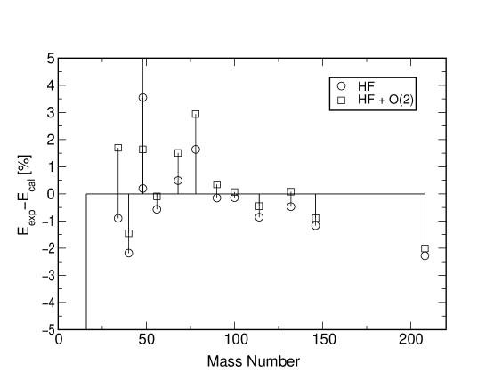
FIG. 3.: Deviation of Hartree-Fock Energy from experiment. Negative errors denote underbinding. Note that ¹⁶O and the second-order result for ⁴⁸Ni are beyond the scale.

FIG. 4.: Second-Order Ground-State Correlation structure in ⁴⁰Ca, ⁴⁸Ca and ²⁰⁸Pb.

FIG. 5.: Charge Form factor in ¹⁶O

FIG. 6.: Charge Form factor in ⁴⁰Ca

FIG. 7.: Charge Form factor in ⁴⁸Ca

FIG. 8.: Charge Form factor in ⁹⁰Zr

FIG. 9.: Charge Form factor in ²⁰⁸Pb

FIG. 10.: Single-particle energies in ⁴⁰Ca compared to experiment [51]

FIG. 11.: Single-particle energies in ²⁰⁸Pb compared to experiment [51]

REFERENCES

- [1] R. Machleidt, K. Holinde and Ch. Elster, Phys. Rep. 149, 1987
- [2] R. B. Wiringa, V. G. J. Stoks and R.Schiavilla, Phys. Rev. C 51, 38 (1995).
- [3] J. Carlson, V. R. Pandharipande, R. B.Wiringa, Nucl. Phys. A 401, 59 (1983).
- [4] V. G. J. Stoks, R. A. M. Klomp, C. P. F. Terheggen and J. J. de Swart, Phys. Rev. C 49, 2950 (1994).
- [5] V. I. Kukulin, V. N. Pomerantsev and Amand Faessler, Phys. Rev. C 59, 3021 (1999).
- [6] R. B. Wiringa, Phys. Rev. C 43,1585 (1991).
- [7] B. S. Pudliner, V. R. Pandharipande J. Carlson, Phys. Rev. C 56, 1730 (1997).
- [8] F. Coester, Nucl. Phys. 7, 421 (1958).
- [9] B. Mihaila, PhD Thesis, University of New Hampshire, 1998
- [10] A. Fabrocini, F. Arias de Saavedra, G. Co’ and P. Folgarait, Phys. Rev. C 57, 1668 (1998).
- [11] D. C. Zheng, B. R. Barrett, J. P. Vary, W. C. Haxton and C.-L. Song, Phys. Rev. C 52, 2488 (1995).
- [12] R. B. Wiringa, Steven C. Pieper, J. Carlson and V. R. Pandharipande, nucl-th/0002022, to be published Phys. Rev. C
- [13] L. Coraggio, A. Covello, A. Gargano, N. Itaco and T. T. S. Kuo, Phys. Rev. C 58, 3346 (1998).
- [14] A. Kerman, Cargése Lectures in Physics, Vol.3 p.396 (1969).
- [15] C. N. Bressel, A. K. Kerman ,B. Rouben, Nucl.Phys. A 124, 624, (1969).
- [16] B. Rouben, PhD Thesis, MIT 1969
- [17] J.Zipse, PhD Thesis, MIT 1970
- [18] E. Riihimäki, PhD Thesis, MIT 1970
- [19] H. A. Bethe, Annu. Rev. Nucl. Sci. 21, 93 (1971).
- [20] D. R. Bés and Z. Szymanski, Nucl.Phys. 28, 42 (1961).
- [21] M. Baranger and K. Kumar, Nucl.Phys. 62, 113 (1965).
- [22] N. H. Kwong and H. S. Köhler, Phys. Rev. C 55, 1650 (1997)
- [23] T. H. R. Skyrme, Phil.Mag. 1, 1043, (1956).
- [24] J. W. Ehlers and S. A. Moszkowski, Phys. Rev. C 6, 217 (1972).
- [25] D. Vautherin and D. M. Brink, Phys. Rev. C 5, 626 (1972).
- [26] J. Decharge and D. Gogny, Phys. Rev. C 21, 1568 (1980).
- [27] P. Quentin and H. Flocard, Annu. Rev. Nucl. Sci. 28, 523 (1978).
- [28] B. D. Serot and J. D. Walecka, Adv. Nucl. Phys. 16, 1 (1986).
- [29] P.-G. Reinhard, Rep. Prog. Phys. 52, 439 (1989).
- [30] J. W. Negele, Phys. Rev. C 5, 1472 (1972).
- [31] B. A. Brown and W. A. Richter, Phys. Rev. C 58, 2099 (1998).
- [32] P. Moller and J. R. Nix, Nucl. Phys. A 536, 20 (1992).
- [33] D. Bohm and D. Pines, Phys. Rev. 92,609 (1953).
- [34] S. E. Koonin, D. J. Dean and K. Langanke, Annu. Rev. Nucl. Part. Sci. 47, 463 (1997).
- [35] G. C. Wick, Phys. Rev. 80, 268 (1950).
- [36] N. M. Hugenholz, Physica 23, 481 (1957).
- [37] M. Gell-Mann and K. A. Brueckner, Phys. Rev. 106, 364 (1957).
- [38] U. S. Mahapatra, B. Datta and D. Mukherjee, J. Phys. Chem. A 103, 1822 (1999)
- [39] J. G. Zabolitsky, Nucl. Phys. A226, 285 (1974).
- [40] E. Chabanat, P. Bonche, P. Haensel, J.Meyer and R. Schaeffer, Nucl.Phys. A627, 710 (1997).
- [41] R. Devi and S. K. Khosa, Phys. Rev. C 54, 1661 (1996).
- [42] B. Blank et al., Phys. Rev. Lett. 84, 1116 (2000).
- [43] R. Schneider, Phys. Scr. T56, 67 (1995).
- [44] M. Chartier et al., Phys. Rev. Lett. 77, 2400 (1996).
- [45] G. Audi and A. H. Wapstra, Nucl. Phys. A 584, 221 (1995).
- [46] M. Bender, K. Rutz, P.-G. Reinhard, J. A. Maruhn, Eur. Phys. J. A 7, 467 (2000).
- [47] M. Beiner, H. Flocard, N. Van Giai, P. Quentin, Nucl. Phys. A 361, 29 (1975)
- [48] J. Dobaczewski, H. Flocard, J. Treiner, Nucl. Phys. A 422, 103 (1984).
- [49] E. Chabanat, Ph. D. Thesis, Lyon (1995).
- [50] P.-G. Reinhard, H. Flocard, Nucl. Phys. A 584, 467 (1995).
- [51] B. Alex Brown, Phys. Rev. C 58, 220 (1998).
- [52] M. Leuschner, J. R. Calarco, F. W. Hersman, E. Jans, G. J. Kramer, L. Lapikás, G. van der Steenhoven, P. K. A. de Witt Huberts, H. P. Blok, N. Kalantar-Nayestanaki, J. Friedrich, Phys. Rev. C 49, 955 (1994).
- [53] S. E. Koonin, PhD Thesis, MIT 1975
- [54] B. H. Brandow, Phys. Rev. 80, 268 (1950).
- [55] G. Fricke et al., At. Data Nucl. Data Tables 60, 177 (1995)
- [56] J. Friedrich and P.-G. Reinhard. Phys. Rev. C 33, 335 (1986).
- [57] A. Bouyssy, J.-F. Mathiot, N. Van Giai, Phys. Rev. C 36, 380 (1987)
- [58] D. Vautherin and M. Veneroni, Phys. Lett. 26B, 552 (1968).
- [59] M. Farine, J. M. Pearson and F. Tondeur, Nucl. Phys., A 615, 135 (1997).
- [60] R. P. Feynman, Phys. Rev. 76, 769 (1949).
- [61] J. Goldstone, Proc. Roy. Soc. A 239, 267 (1957)