Diabatic Mean-Field Description of Rotational Bands
in Terms of the Selfconsistent Collective Coordinate Method

1 Introduction

Back-bending of the yrast rotational bands is one of the most striking phenomena in the spectroscopic studies of rapidly rotating nuclei.[1, 2]  The first back-bending, which has been observed systematically in the rotational bands of the rare-earth nuclei, has been understood as a band-crossing between the ground state rotational band ($g$-band) and the lowest two quasineutron excited band ($s$-band). A simple approach to describe the band-crossing is the cranked mean-field approximation, where the concept of independent particle motion in the rotating frame is fully employed. As long as the conventional (adiabatic) cranking model is used, however, the two bands mix at the same rotational frequency and, in the crossing region, loose their identities as individual rotational bands. It should be noted that the difficulty lies in the fact that the angular momenta of two bands are considerably different in the vicinity of the crossing frequency where the mixing takes place, especially in the case of sharp back-bendings, and such a mixing is largely unphysical.[3, 4, 5]

A key to solve this problem is to construct diabatic rotational bands, where the internal structure of the band does not change abruptly.[6, 7, 8, 9]  Once reliable diabatic bands are obtained it is rather straightforward to mix them if the number of independent bands are few as in the case of the first back-bending. Note, however, that it is highly non-trivial how to construct reliable diabatic bands in the mean-field approximation, because it is based on the variational principle and the mixing at the same rotational frequency is inevitable for states with the same quantum numbers (in the intrinsic frame). On the other hand, in the mean-field approximation, the effects of rotational motion on the internal structure of the $g$-band can be nicely taken into account as selfconsistent changes of the deformation and the pairing gap parameters. Furthermore, rotation alignment effects of the quasiparticle angular momenta are described in a simple and clear way. Therefore, it is desired to develop a method to describe the rotational band diabatically within the mean-field approximation.

In this paper, we present a powerful method to obtain reliable diabatic rotational bands by making use of the selfconsistent collective coordinate (SCC) method.[10]  The method is applied to the $g$- and $s$-bands and the results for nuclei in the rare-earth region are compared systematically with experimental data. In order to reproduce the rotational spectra, the choice of residual interaction is essential. We use the pairing-plus-quadrupole force type interaction.[11]  However, it has been well-known that the moment of inertia is generally underestimated by about 20$-$30% if only the monopole-pairing interaction is included.[12]  Therefore, we exploit the monopole and quadrupole type interaction in the pairing channel, and investigate the best form of the quadrupole-pairing part. This is done in §2. After fixing the suitable residual interaction, we present in §3 a formulation to describe the diabtic rotational bands and results of its application to nuclei in the rare-earth region. In practical applications it often happens that a complete set of the diabatic quasiparticle basis is necessary; for example, in order to go beyond the mean-field approximation. For this purpose, we present in §4 a practical method to construct the diabatic quasiparticle basis satisfying the orthonormality condition. Concluding remarks are given in §5.

2 Quadrupole-pairing interaction suitable for deformed nuclei

In this section we try to fix the form of residual interactions, which is suitable to describe the properties of deformed rotating nuclei. It might be desirable to use effective interactions like Skyrme-type interactions,[13]  but that is out of scope of the present investigation. We assume the separable-type schematic interactions instead, and try to fix their forms and strengths by a global fit of the basic properties; the even-odd mass difference and the moment of inertia.

2.1 Residual interactions

The residual interaction we use in the present work is of the following form:

$$V=-G_{0}P_{00}^{\dagger}P_{00}-G_{2}\sum_{K}P_{2K}^{\dagger}P_{2K}-{1\over 2}\,\sum_{K}\mathchar 28948\relax_{2K}Q_{2K}^{\dagger}Q_{2K},$$ (2.1)

where the first and the second terms are the monopole- and quadrupole-pairing interactions, while the third term is the quadrupole particle-hole type interaction. The pairing interactions are set up for neutrons and protons separately (the $T=1$ and $T_{z}=\pm 1$ pairing) as usual, although it is not stated explicitly, and only the isoscalar part is considered for the quadrupole interaction. The quadrupole-pairing interaction is included for purpose of better description of moment of inertia: It has been known for many years[12] that the cranking moments of inertia evaluated taking into account only the monopole-pairing interaction underestimate the experimental ones systematically in the rare-earth region, as long as the monopole-pairing strength is fixed to reproduces the even-odd mass differences. It should be mentioned that the treatment of residual interactions in the pairing and the particle-hole channels are different: In the pairing channel the mean-field (pairing gap) is determined by the interaction selfconsistently, while that in the particle-hole channel (spatial deformation) is obtained by the Nilsson-Strutinsky method[14, 15] and the interaction in this channel only describes the dynamical effects, i.e. the fluctuations around the equilibrium mean-field.

The basic quantity for deformed nuclei is the equilibrium deformation. For the present investigation, where the properties of deformed rotational nuclei are systematically studied, the Nilsson-Strutinsky method is most suitable to determine the equilibrium deformations, because there is no adjustable parameters. As emphasized by Kishimoto and Sakamoto,[17]  the particle-hole type quadrupole interaction for deformed nuclei should be of the double-stretched form:[17, 18, 19]

$$Q_{2K}=\sum_{ij}q_{2K}(ij)\,c_{i}^{\dagger}c_{j},\quad q_{2K}(ij)=\langle i|(r^{2}Y_{2K})^{\prime\prime}|j\rangle,$$ (2.2)

where $c_{i}^{\dagger}$ is the nucleon creation operator in the Nilsson state $|i\rangle$. $(O)^{\prime\prime}$ means that the Cartesian coordinate in the operator $O$ should be replaced such as $x_{k}\rightarrow x^{\prime\prime}_{k}\equiv(\mathchar 28961\relax_{k}/\mathchar 28961\relax_{0})x_{k}$ ($k=x,y,z$), where $\mathchar 28961\relax_{x}$, $\mathchar 28961\relax_{y}$ and $\mathchar 28961\relax_{z}$ are frequencies of the anisotropic oscillator potential and related to the deformation parameter $(\mathchar 28943\relax_{2},\mathchar 28941\relax)$;[15, 16]  here $\hbar\mathchar 28961\relax_{0}\equiv\hbar(\mathchar 28961\relax_{x}\mathchar 28961\relax_{y}\mathchar 28961\relax_{z})^{1/3}=41.0/A^{1/3}$ MeV ($A$ is the mass number). Then the selfconsistent condition gives, at the equilibrium shape, a vanishing mean value for the double-stretched quadrupole operator, $\langle Q_{2K}\rangle=0$, and thus the meaning of residual interaction is apparent for the double-stretched interaction. Moreover, the force strengths are determined at the same time to be the so-called selfconsistent value,

$$\mathchar 28948\relax_{2K}=\mathchar 28948\relax_{2}^{\rm self}={4\mathchar 28953\relax\over 3}{\hbar\mathchar 28961\relax_{0}\over AR^{2}_{0}b^{2}_{0}},\quad{\rm with}\quad b^{2}_{0}={\hbar\over M\mathchar 28961\relax_{0}},\;\;R_{0}=1.2A^{1/3}\;{\rm fm},$$ (2.3)

by which the $\mathchar 28940\relax$- and $\mathchar 28941\relax$-vibrational excitations are correctly described. Strictly speaking, the vanishing mean value of $Q_{2K}$ holds only for the harmonic oscillator model. It is, however, easily confirmed that the mean value vanishes in a good approximation in the case of Nilsson potential. In fact the calculated ratio of mean values of the double-stretched and non-stretched quadrupole operator is typically within few percent, if the deformation parameter determined by the Strutinsky procedure is used.

Pairing correlations are important for the nuclear structure problem as well. The operators entering in the pairing type residual interactions are of the form

$$P_{00}^{\dagger}=\sum_{i>0}c_{i}^{\dagger}c_{\tilde{i}}^{\dagger},\quad P_{2K}^{\dagger}=\sum_{ij>0}p_{2K}(ij)\,c_{i}^{\dagger}c_{\tilde{j}}^{\dagger},$$ (2.4)

where ${\tilde{j}}$ denotes the time-reversal conjugate of the Nilsson state $j$. In contrast to the residual interactions in the particle-hole channel, there is no such selfconsitency condition known in the pairing channel. Therefore, we use the Hartree-Bogoliubov (HB) procedure (exchange terms are neglected) for the pairing interactions, only the monopole part of which leads to the ordinary BCS treatment. Note that the generalized Bogoliubov transformation is necessary in order to treat the quadrupole-pairing interaction, since the pairing potential becomes state-dependent and contains non-diagonal elements:

$$\mathchar 28929\relax_{ij}=\mathchar 28929\relax_{00}\,\mathchar 28942\relax_{ij}+\sum_{K}\mathchar 28929\relax_{2K}\,p_{2K}(ij),$$ (2.5)

where $\mathchar 28929\relax_{00}=G_{0}\,\langle P_{00}\rangle$ and $\mathchar 28929\relax_{2K}=G_{2}\,\langle P_{2K}\rangle$, the expectation values being taken with respect to the resultant HB state.

For the application of these residual interaction we are mainly concerned with deformed nuclei in the rare-earth region, where the neutron and proton numbers are considerably different. In such a case, the “iso-stretching” of multipole operators,[20, 21]  $Q_{\mathchar 28956\relax}\rightarrow(2N_{\mathchar 28956\relax}/A)^{2/3}\,Q_{\mathchar 28956\relax}$ for $\mathchar 28956\relax=\mathchar 28951\relax,\mathchar 28953\relax$ ($N_{\mathchar 28956\relax}$ denotes the neutron or proton number and $A$ the mass number), is necessary in accordance with the difference of the oscillator frequencies, $\mathchar 28961\relax_{0}^{\mathchar 28956\relax}=(2N_{\mathchar 28956\relax}/A)^{1/3}\mathchar 28961\relax_{0}$, or of the oscillator length, $(b_{0}^{\mathchar 28956\relax})^{2}=(2N_{\mathchar 28956\relax}/A)^{-1/3}b^{2}_{0}$. We employ this modification for the quadrupole interaction in the particle-hole channel.

2.2 Treatment of pairing interactions

As for the quadrupole-pairing part, there are at least three variants that have been used in the literature.[22, 23, 24, 25, 26, 27]  Namely, they are non-stretched, single-stretched and double-stretched quadrupole-pairing interactions, where the pairing form factor in the operator in Eq. (2.4) is defined as,

$$p_{2K}(ij)=\langle i|r^{2}Y_{2K}|j\rangle,\,\,\,\langle i|(r^{2}Y_{2K})^{\prime}|j\rangle,\,\,\,\langle i|(r^{2}Y_{2K})^{\prime\prime}|j\rangle,$$ (2.6)

respectively. The single-stretching of operators is analogously performed by the replacement, $x_{k}\rightarrow x^{\prime}_{k}\equiv\sqrt{\mathchar 28961\relax_{k}/\mathchar 28961\relax_{0}}~{}x_{k}$ ($k=x,y,z$). Note that there are matrix elements between the Nilsson states with $\mathchar 28929\relax N_{\rm osc}=\pm 2$ in Eq. (2.6). We have neglected them in the generalized Bogoliubov transformation in accordance with the treatment of the Nilsson potential, which is arranged to have vanishing matrix elements of $\mathchar 28929\relax N_{\rm osc}=\pm 2$.

Consistently to the Nilsson-Strutinsky method, we use the smoothed pairing gap method[14] in which the monopole-pairing force strength is determined for a given set of single-particle energies by

$${2\over G_{0}}={1\over 2}\,{\widetilde{g}}_{\rm F}\log{\Bigl{(}\mathchar 28931\relax/{\widetilde{\mathchar 28929\relax}}+\sqrt{(\mathchar 28931\relax/{\widetilde{\mathchar 28929\relax}})^{2}+1}\,\Bigr{)}},$$ (2.7)

where ${\widetilde{g}}_{\rm F}$ is the Strutinsky smoothed single-particle level density at the Fermi surface, $\mathchar 28931\relax$ is the cutoff energy of pairing model space, for which we use $\mathchar 28931\relax=1.2\hbar\mathchar 28961\relax_{0}$, and ${\widetilde{\mathchar 28929\relax}}$ is the smoothed pairing gap. We introduce a parameter $d$ (MeV) to control the strength of the monopole-pairing force by

$${\widetilde{\mathchar 28929\relax}}={d\over\sqrt{A}},$$ (2.8)

through Eq. (2.7), where the same smoothed pairing gap is used for both neutrons and protons, for simplicity. As for the quadrupole-pairing force strength, we take the following form,

$$G_{2}=G_{0}\,{g_{2}\over R^{4}_{0}},\quad{\rm with}\quad R_{0}=1.2A^{1/3}\;{\rm fm}.$$ (2.9)

Thus, we have two parameters $d$ (in MeV) and $g_{2}$ for the residual interactions in the pairing channel.

It is worthwhile mentioning that Eq. (2.7) gives the form,

$$G^{\mathchar 28956\relax}_{0}\approx{c\over A}\Bigl{(}{2N_{\mathchar 28956\relax}\over A}\Bigr{)}^{-1/3},\quad{\rm with}\quad c={41.0\over 3^{2/3}2^{4/3}}\log{\bigl{(}2\mathchar 28931\relax/{\widetilde{\mathchar 28929\relax}}\bigr{)}},$$ (2.10)

for the semiclassical treatment of the isotropic harmonic oscillator model,[28, 29]  where ${\widetilde{g}}_{\rm F}^{\mathchar 28956\relax}\approx(3N)^{2/3}/(\hbar\mathchar 28961\relax_{0}^{\mathchar 28956\relax})$, and it is a good approximation for the Nilsson potential. The quantity $\log{\bigl{(}2\mathchar 28931\relax/{\widetilde{\mathchar 28929\relax}}\bigr{)}}$ depends very slowly on the mass number and can be replaced by a representative value for a restricted region of mass table. Taking $A=170$, one obtains $c\approx 23$, which gives the monopole-pairing force strength often used for nuclei in the rare-earth region.

2.3 Determination of parameters $d$ and $g_{2}$

Now let us determine the form of the quadrupole-pairing interaction. Namely, we would like to answer the question of which form factor in Eq. (2.6) is best, and of what are the values of the parameters, $d$ and $g_{2}$, introduced in the previous subsection. For this purpose, we adopt the following criteria; the moments of inertia ${\cal J}_{0}$ of the Harris formula[30] and the even-odd mass differences (the third order formula[28]) for even-even nuclei should be simultaneously reproduced as good as possible. Since the neutron contribution is more important for the moment of inertia, we have used the even-odd mass difference for neutrons, $E_{\mathchar 28951\relax}^{({{\rm e}\hbox{\raise-0.45206pt\hbox{\rm-}}{\rm o}})}$. Then it turns out that the proton even-odd mass difference is also reasonably well reproduced as long as the same smoothed pairing gap is used for neutrons and protons. Thus, the two parameters $d$ (MeV) and $g_{2}$ are searched so as to minimize the root-mean-square deviations of these quantities divided by their average values,

$$X_{\rm rms}(x)=\Bigl{[}{1\over N_{\rm data}}\sum_{i=1}^{N_{\rm data}}\bigl{(}x_{i}^{({\rm exp})}-x_{i}^{({\rm cal})}\bigr{)}^{2}\Bigr{]}^{1/2}{\hbox{$\left/\vbox to0.0pt{}\right.\n@space$}}\,\Bigl{[}{1\over N_{\rm data}}\sum_{i=1}^{N_{\rm data}}x_{i}^{({\rm exp})}\Bigr{]}$$ (2.11)

for $x={\cal J}_{0}$ and $E_{\mathchar 28951\relax}^{({{\rm e}\hbox{\raise-0.45206pt\hbox{\rm-}}{\rm o}})}$. Nuclei used in the search are chosen from even-even rare-earth nuclei in Table I, thus $N_{\rm data}=83$ (58) for $x=E_{\mathchar 28951\relax}^{({{\rm e}\hbox{\raise-0.45206pt\hbox{\rm-}}{\rm o}})}$ (${\cal J}_{0}$).

Table I: Nuclei included for the search of the pairing interaction parameters, $d$ and $g_{2}$.

	64Gd	66Dy	68Er	70Yb	72Hf	74W
$N$ for $E_{\mathchar 28951\relax}^{({{\rm e}\hbox{\raise-0.45206pt\hbox{\rm-}}{\rm o}})}$	76$-$100	78$-$102	80$-$104	80$-$108	84$-$110	86$-$114
$N$ for ${\cal J}_{0}$	86$-$96	86$-$100	86$-$102	86$-$108	90$-$110	92$-$114

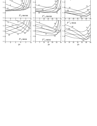
Fig. 1: Root-mean-square deviations of neutron even-odd mass differences and moments of inertia, calculated by using the non-stretched (left), single-stretched (middle), and double-stretched (right) residual quadrupole-pairing interactions. The upper panels shows the results for ${\overline{X}}_{\rm rms}$ and the lower panels for $X_{\rm rms}^{\rm M}$, see Eqs. (2.12) and (2.13). They are calculated as functions of the two parameters $d$ and $g_{2}$. Each curve is drawn with a fixed value of $d$ (MeV), which is attached near the curve, as a function of $g_{2}$.

Note that the neutron even-odd mass difference has been calculated in the same way as the experimental data by taking the third order difference of calculated binding energies for even and odd $N$ nuclei, where the blocking HB calculation has been done for odd-mass nuclei. In the Nilsson-Strutinsky method the grid of deformation parameters $-0.08\leq\mathchar 28943\relax_{2}\leq 0.40$ and $-0.08\leq\mathchar 28943\relax_{4}\leq 0.12$ with an interval of $0.04$ are used. The $ls$ and $ll$ parameters of the Nilsson potential are taken from Ref. ?. We have assumed the axial symmetry in the calculation of this subsection since only the ground state properties are examined. Experimental binding energies are taken from the 1993 Atomic Mass Evaluation.[32]  As for the experimental moment of inertia, the Harris parameters, ${\cal J}_{0}$ and ${\cal J}_{1}$, are calculated from the observed excitation energies of the $2^{+}$ and $4^{+}$ states belonging to the ground state band, experimental data being taken from Ref. ? and the ENSDF database.[34]  If the value of ${\cal J}_{0}$ calculated in this way becomes negative or ${\cal J}_{1}$ greater than 1000 $\hbar^{4}$/MeV³ (this happens for near spherical nuclei), then ${\cal J}_{0}$ is evaluated by only using the $2^{+}$ energy, i.e. by $3/E_{2^{+}}$. The Thouless-Valtion moment of inertia,[35]  which includes the effect of the $K=1$ component of the residual quadrupole-pairing interaction, is employed as the calculated moment of inertia. Here, again, the matrix elements between states with $\mathchar 28929\relax N_{\rm osc}=\pm 2$ are neglected for simplicity in the same way as in the step of diagonalization of the mean-field Hamiltonian. The contributions of them are rather small for the calculation of moment of inertia, since the $\mathchar 28929\relax N_{\rm osc}=\pm 2$ matrix elements of the angular momentum operator are smaller than the $\mathchar 28929\relax N_{\rm osc}=0$ ones by a factor $\approx\mathchar 28943\relax_{2}$ and the energy denominators are larger. We have checked that those effects are less than 5 % for the Thouless-Valatin moment of inertia in well deformed nuclei.

In Fig. 1 we show root-mean-square deviations of the result of calculation for neutron even-odd mass differences and moments of inertia. We have found that the behaviors of these two quantities, $X_{\rm rms}(E_{\mathchar 28951\relax}^{({{\rm e}\hbox{\raise-0.45206pt\hbox{\rm-}}{\rm o}})})$ and $X_{\rm rms}({\cal J}_{0})$, as functions of $g_{2}$ with fixed $d$ are opposite, and so the mean value

$${\overline{X}}_{\rm rms}={1\over 2}\,\bigl{(}X_{\rm rms}(E_{\mathchar 28951\relax}^{({{\rm e}\hbox{\raise-0.45206pt\hbox{\rm-}}{\rm o}})})+X_{\rm rms}({\cal J}_{0})\bigr{)}$$ (2.12)

become almost constant, especially for the case of the non-stretched quadrupole-pairing. Therefore, we also display the results for the maximum among the two,

$$X_{\rm rms}^{\rm M}={\rm max}\bigl{\{}X_{\rm rms}(E_{\mathchar 28951\relax}^{({{\rm e}\hbox{\raise-0.45206pt\hbox{\rm-}}{\rm o}})}),\,X_{\rm rms}({\cal J}_{0})\bigr{\}}.$$ (2.13)

As is clear from Fig. 1, the best fit is obtained for the double-stretched quadrupole-pairing interaction with $d=14$ (MeV) and $g_{2}=30$. It should be mentioned that the value of $g_{2}$ is close to the one $g_{2}=28\mathchar 28953\relax/3$ in Ref. ?, where it is derived from the multipole decomposition of the $\mathchar 28942\relax$-interaction and this argument is equally applicable if the double-stretched coordinate is used in the interaction. It is interesting to notice that if the non-stretched or the single-stretched quadrupole-pairing interaction is used, then one cannot make either ${\overline{X}}_{\rm rms}$ or $X_{\rm rms}^{\rm M}$ smaller than 0.2. ${\overline{X}}_{\rm rms}$ in the non-stretched case is rather flat as a function of $g_{2}$ and the minimum occurs at $d=12$ (MeV) and $g_{2}=0$ (no quadrupole-pairing). $X_{\rm rms}^{\rm M}$ in the non-stretched case takes the minimum at small quadrupole-pairing, $d=12$ (MeV) and $g_{2}=2$. Both ${\overline{X}}_{\rm rms}$ and $X_{\rm rms}^{\rm M}$ are flat as a function of $g_{2}$ also in the single-stretched case, and take the minimum at $d=12$ (MeV) and $g_{2}=16$. In contrast, the double-stretched interaction gives well developed minima for both ${\overline{X}}_{\rm rms}$ and $X_{\rm rms}^{\rm M}$. These results clearly show that one has to use the double-stretched quadrupole-pairing interaction.

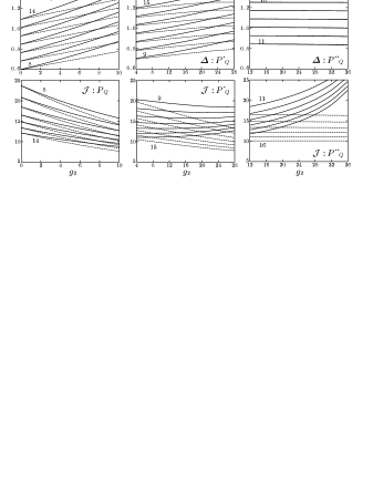
Fig. 2: Pairing gaps (upper panels) and moments of inertia (lower panels), calculated by using the non-stretched (left), single-stretched (middle), and double-stretched (right) residual quadrupole-pairing interactions. Average pairing gaps ${\overline{\mathchar 28929\relax}}$ and monopole-pairing gaps $\mathchar 28929\relax_{00}$ (MeV), see Eq. (2.14), are displayed by solid and dashed curves, respectively, in the upper panels, while Thouless-Valatin and Belyaev moments of inertia ($\hbar^{2}$/MeV) (c.f. Eq. (3.78)) are displayed as solid and dashed curves, respectively, in the lower panels. They are calculated as functions of the two parameters $d$ and $g_{2}$. Each curve is drawn with a fixed value of $d$ (MeV), which is attached near the curve and changed by step of 1 MeV, as a function of $g_{2}$. The calculation has been done for a typical deformed nucleus, ¹⁶⁸Yb, with deformation parameters $(\mathchar 28943\relax_{2},\,\mathchar 28943\relax_{4})=(0.2570,\,0.0162)$.

One may wonder why the non- and single-stretched interactions do not essentially improve the root-mean-square deviations. The quadrupole-pairing interaction affects $E_{\mathchar 28951\relax}^{({{\rm e}\hbox{\raise-0.45206pt\hbox{\rm-}}{\rm o}})}$ and ${\cal J}_{0}$ in two ways: One is the static (mean-field) effect through the change of static pairing potential (2.5), and the other is a dynamical effect (higher order than the mean-field approximation) and typically appears as the Migdal term in the Thouless-Valatin moment of inertia (c.f. Eq. (3.78) and (3.79)). The former effect can be estimated by the averaged pairing gap,

$${\overline{\mathchar 28929\relax}}=\sum_{i}\mathchar 28929\relax_{ii}\,/\,\sum_{i}1=\mathchar 28929\relax_{00}+\sum_{K}\mathchar 28929\relax_{2K}\sum_{i}p_{2K}(ii)\,/\,\sum_{i}1,$$ (2.14)

where the summation is taken over the Nilsson basis state $i$’s included in the pairing model space. Stronger quadrupole-pairing interaction results in larger ${\overline{\mathchar 28929\relax}}$, which leads to the increase of even-odd mass difference on one hand and the reduction of moment of inertia on the other hand. The Migdal term coming from the $K=1$ component of the quadrupole-pairing interaction makes the moment of inertia larger when the force strength is increased. Therefore, the moment of inertia either increases or decreases as a function of force strength, depending on which effect is stronger. In Fig. 2, we have shown the energy gap and the moment of inertia for a typical rare-earth deformed nuclei ¹⁶⁸Yb as functions of the two parameters $d$ and $g_{2}$ in parallel with Fig. 1. One can see that the average as well as monopole-pairing gaps increase rapidly as functions of the quadrupole-pairing strength if the non-stretched interaction is used. This static effect is so strong that the Thouless-Valatin moment of inertia decreases. In the case of the single-stretched case, similar trend is observed for the pairing gap, though it is not so dramatic as in the case of non-stretched interaction. The static effect almost cancels out the dynamical effect and then the Thouless-Valatin moment of inertia stays almost constant against $g_{2}$ in this case. On the other hand, if one uses the double-stretched interaction, the pairing gap stays almost constant as a function of $g_{2}$. This is because $\langle P_{2K}\rangle\approx 0$ holds in a very good approximation, which is in parallel with the fact that the quadrupole equilibrium shape satisfies the selfconsistent condition, $\langle Q_{2K}\rangle=0$, for the double-stretched quadupole operator. Thus the effect of the double-stretched quadrupole-pairing interaction plays a similar role as the particle-hole interaction channel; it acts as a residual interaction and does not contribute to the static mean-field.

2.4 Results of calculation

It has been found in the previous subsection that the double-stretched form of the quadrupole-pairing interaction with parameters $d=14$ MeV and $g_{2}=30$ gives best fitting for the even-odd mass differences and the moments of inertia in the rare-earth region. Resulting root-mean-square deviations are $X_{\rm rms}(E_{\mathchar 28951\relax}^{({{\rm e}\hbox{\raise-0.45206pt\hbox{\rm-}}{\rm o}})},\,{\cal J}_{0})=(0.115,\,0.136)$. If one uses $(d,g_{2})=(13,28)$ or $(12,20)$, as examples, those quantities become $X_{\rm rms}(E_{\mathchar 28951\relax}^{({{\rm e}\hbox{\raise-0.45206pt\hbox{\rm-}}{\rm o}})},\,{\cal J}_{0})=(0.154,\,0.127)$ or $(0.235,\,0.121)$, respectively. Therefore, making the two quantities smaller is complementary as discussed in §2.3.

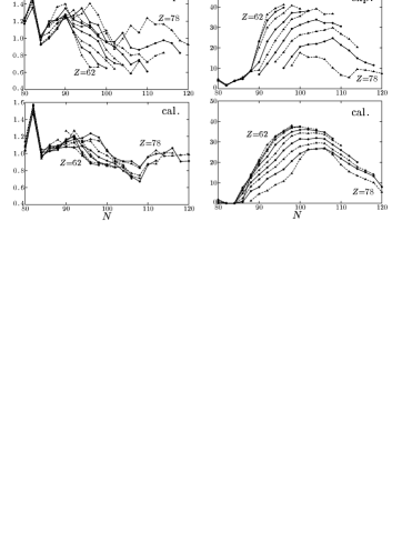
Fig. 3: Comparison of calculated even-odd mass differences (left panels, in MeV) and moments of inertia (right panels, in $\hbar^{2}$/MeV) with experimental data for nuclei in the rare-earth region. Experimental data are displayed in the upper panels while the calculated ones in the lower panels. Isotopes with $Z=62-78$ are connected by solid ($Z=0$ mod 4) or dashed ($Z=2$ mod 4) curves as functions of neutron number $N$. The double-stretched quadrupole-pairing interaction is used with parameters $d=14$ MeV and $g_{2}=30$.

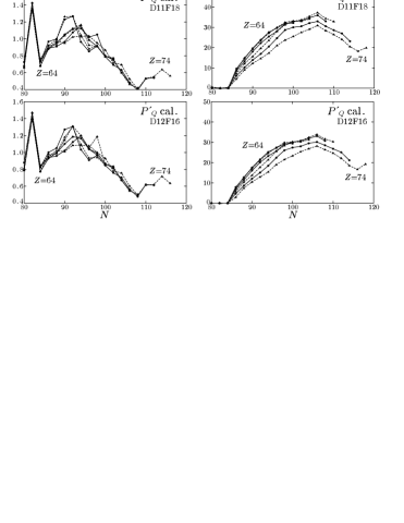
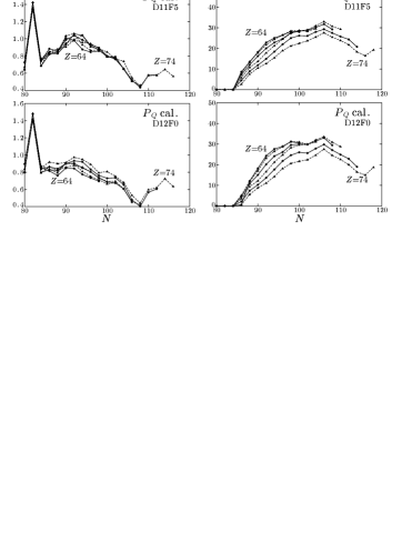
Fig. 4: Even-odd mass differences (left panels) and moments of inertia (right panels) for $Z=64-74$ isotopes, calculated by using the single- and non-stretched quadrupole-pairing interactions. The panels from top to bottom show the results of the single-stretched cases with parameters ($d=11$ MeV, $g_{2}=18$) and ($d=12$ MeV, $g_{2}=16$), and of the non-stretched cases with parameters ($d=11$ MeV, $g_{2}=5$) and ($d=12$ MeV, $g_{2}=0$), respectively.

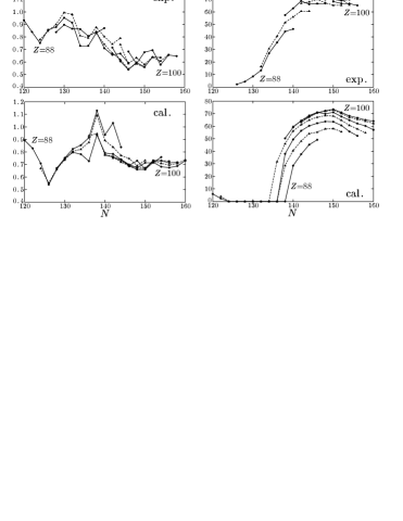
Fig. 5: Same as Fig. 3, but for nuclei in the actinide region. Isotopes with $Z=88-100$ are connected by solid ($Z=0$ mod 4) or dashed ($Z=2$ mod 4) curves as functions of neutron number $N$.

We compare the results of calculation with experimental data in Fig. 3 as functions of neutron number. In this calculation the results of Sm ($Z=62$), Os ($Z=76$) and Pt ($Z=78$) isotopes are also included, which are not taken into account in the fitting procedure. As is clear from the figure, both even-odd mass differences and moments of inertia are not well reproduced in heavy Os and Pt isotopes; especially even-odd mass differences are underestimated by about 20%, and moments of inertia overestimated by about up to 50% in Pt nuclei with $N\mathrel{\hbox{\raise 0.86108pt\hbox{$>$}\kern-7.5pt\raise-3.87495pt\hbox{$\sim$}}}100$. In these nuclei, low-lying spectra suggest that they are $\mathchar 28941\relax$-unstable, and therefore correlations in the $\mathchar 28941\relax$ degrees of freedom are expected to play an important role. Except for these nuclei, the overall agreements have been achieved, particularly for deformed nuclei with $N\approx 90-100$. It is, however, noted that some features seen in experimental data are not reproduced in the calculation: (1) The maximum at $N=90$ and the minimum at $N=106$ or $110$ in the even-odd mass difference are shifted to $N=92$ and $N=98$, respectively. This is because details of the neutron single-particle level spacings in the present Nilsson potential are slightly inadequate. (2) The proton number dependences of both the even-odd mass difference and the moment of inertia are too weak: curves of both quantities bunch more strongly in the calculation. This trend is clearer in light $Z$ nuclei, $Z\leq 68$, for example, Gd or Dy; the even-odd mass difference in these isotopes decreases more slowly as a function of neutron number in the calculation, which results in the slower increase of the moment of inertia. This problem suggests that some neutron-proton correlations might be necessary.

For comparison sake, results obtained by using the quadrupole-pairing interactions of the single-stretched and the non-stretched types are displayed in Fig. 4. In the calculation of the single-stretched case, the values of the two parameters, $d=11$ MeV and $g_{2}=18$, are employed, resulting $X_{\rm rms}(E_{\mathchar 28951\relax}^{({{\rm e}\hbox{\raise-0.45206pt\hbox{\rm-}}{\rm o}})},\,{\cal J}_{0})=(0.240,\,0.170)$, in one case, and the values $d=12$ MeV and $g_{2}=16$, resulting $X_{\rm rms}(E_{\mathchar 28951\relax}^{({{\rm e}\hbox{\raise-0.45206pt\hbox{\rm-}}{\rm o}})},\,{\cal J}_{0})=(0.192,\,0.214)$, in another case. Comparing with the experimental data in Fig. 3, the decrease of even-odd mass difference with neutron number is too strong, while the increase of moment of inertia near $N\approx 90$ is too slow. In the calculation of non-stretched case, the values of the two parameters, $d=11$ MeV and $g_{2}=5$ are employed, resulting $X_{\rm rms}(E_{\mathchar 28951\relax}^{({{\rm e}\hbox{\raise-0.45206pt\hbox{\rm-}}{\rm o}})},\,{\cal J}_{0})=(0.257,\,0.237)$, in one case, and the values $d=12$ MeV and $g_{2}=0$, resulting $X_{\rm rms}(E_{\mathchar 28951\relax}^{({{\rm e}\hbox{\raise-0.45206pt\hbox{\rm-}}{\rm o}})},\,{\cal J}_{0})=(0.265,\,0.204)$, in another case. The average values of the even-odd mass difference are considerably smaller and those of the moment of inertia are 20$-$30% smaller compared to the experimental data. Note that the last case ($d=12$ MeV and $g_{2}=0$) is nothing but the calculation without the quadrupole-pairing interaction. The trend of weak proton number dependence does not change for all three forms of the quadrupole-pairing interaction.

The merit of the Nilsson-Strutinsky method is that a global calculation is possible once the mean-field potential is given. We have then performed the calculation for nuclei in the actinide region with the same pairing interaction and the parameters as in the rare-earth region, i.e. the double-stretched quadrupole-pairing with $d=14$ MeV and $g_{2}=30$. The result is shown in Fig. 5. Nuclei in the light actinide region are spherical or weakly deformed with possible octupole deformations. The experimental moments of inertia suggest that nucleus in this region begins to deform at $N\approx 134$, and gradually increases the deformation until a rather stable deformation is established at $N\mathrel{\hbox{\raise 0.86108pt\hbox{$>$}\kern-7.5pt\raise-3.87495pt\hbox{$\sim$}}}140$. In the nuclei with $N=88$ and $90$, the neutron number at which the deformation starts to grow is too large in the calculation, and the even-odd mass differences take considerably different behaviour from the experimental data. This disagreement possibly suggests the importance of octupole correlations. Except for these difficiencies, both even-odd mass differences and moments of inertia in heavy well-deformed nuclei are very well reproduced in the calculation. It should be emphasized that the parameters fixed in §2.3 for the rare-earth region are equally well applicable for the actinide region.

3 SCC method for constructing diabatic rotational bands

The SCC method[10] is a theory aiming at microscopic description of large amplitude collective motions in nuclei. The rotational motion is one of the most typical large amplitude motions. Therefore it is natural to apply the SCC method to the nuclear collective rotation. In Ref. ?, this line has been put into practice for the first time in order to obtain the diabatic rotational bands, where the interband interaction associated with the quasiparticle alignments is eliminated. It has also been shown that the equation of path in the SCC method leads to the selfconsistent cranking model in the case of rotational motion. Corresponding to the uniform rotation about one of the principal axes of nuclear deformation, the one-dimensional rotation has been considered as in the usual cranking model. We keep this basic feature in the present work.

More complete formulation and its application to the ground state rotational bands ($g$-bands) in realistic nuclei have been done in Ref. ?, followed by further applications to the Stockholm bands ($s$-bands)[38] and improved calculations with including the quadurpole-pairing interaction.[39]  In these works the basic equations of the SCC method have been solved in terms of the angular momentum expansion ($I$-expansion). Thus, the $A$ and $B$ parameters in the rotational energy expansion, $E(I)=A\,I(I+1)+B\,[I(I+1)]^{2}$, have been studied in detail. It is, however, well known that applicability of the $I$-expansion is limited to relatively low-spin regions. This limitation is especially severe in the case of the $s$-bands: One has to take the starting angular momentum $I_{0}$ ($\approx 10\hbar$[38]) and the expansion in terms of $(I-I_{0})$ is not very stable. Because of this problem comparisons with experimental data have not been possible for the $s$-bands.[38]  In the present study, the rotational frequency expansion is utilized instead, according to the original work.[36]  Then the diabatic cranking model is naturally derived. Thus, after obtaining the diabatic quasiparticle states, we construct the $s$-band as the two quasiparticle aligned band on the vacuum $g$-band at given rotation frequencies. This is precisely the method of the cranked shell model,[40]  which has been established as a powerful method to understand the high-spin rotational bands accompanying quasiparticle excitations.

Another important difference of the present work from Refs. ?, ?, ? is that the expansion method based on the normal modes of the random phase approximation (RPA) is used for solving the basic equations in these references. The method is very convenient to investigate detailed contents of the rotation-vibration couplings, e.g. how each normal mode contributes to the rotational $A$ and/or $B$ parameters, as has been discussed in Refs. ?, ?. On the other hand, we are aiming at a systematic study of rotational spectra of both $g$- and $s$-bands in the rare-earth region. Then the use of the RPA response-function matrix is more efficient for such a purpose, because it is not necessary to solve the RPA equation for all the normal modes explicitly.

It has to be mentioned that the problem of nucleon number conservation, i.e. the pairing rotation, can be treated similarly.[41]  Actually, if the SCC method is applied to the spatial rotational motion, the mean value of the nucleon number changes as the angular momentum or the rotational frequency increases. A proper treatment of the pairing rotations is required, i.e. the coupling of the spatial and pairing rotations should be included.[41]  However, it has been found[37] that the effect of the coupling is negligibly small for the case of the rotational motion in well deformed nuclei. Therefore, we simply neglect the proper treatment of the nucleon number in the following.

Although it is not the purpose of this paper to review applications of the SCC method to other nuclear structure phenomena, we would here like to cite a brief review[42] and some papers, in which low-frequency quadrupole vibrations are analyzed on the basis of the SCC method: anharmonic gamma vibrations,[43, 44, 45]  shape phase transitions in Sm isotopes,[46, 47, 48]  anharmonicities of the two phonon states in Ru and Se isotopes,[49]  single-particle levels and configurations in the shape phase transition regions,[50]  and a derivation of the Bohr-Mottelson type collective Hamiltonian and its application to transitional Sm isotopes.[51]

3.1 Basic formulation

The starting point of the SCC method is the following time-dependent Hartree-Bogoliubov (TDHB) mean-field state

$$|\mathchar 28958\relax(\mathchar 28946\relax,I_{x})\rangle=W(\mathchar 28946\relax,I_{x})|\mathchar 28958\relax_{0}\rangle,$$ (3.1)

which is parametrized by the time-dependent collective variables $\mathchar 28946\relax(t)$ and $I_{x}(t)$ through the unitary transformation $W(\mathchar 28946\relax,I_{x})$ from the ground (non-rotating) state $|\mathchar 28958\relax_{0}\rangle$. In the case of rotational motion, $I_{x}$ corresponds to the angular momentum about the rotating axis $x$, which is a conserved quantity, and $\mathchar 28946\relax$ is the conjugate angle variable around the $x$-axis. In order to guarantee the rotational invariance, $W(\mathchar 28946\relax,I_{x})$ has to be of the form

$$W(\mathchar 28946\relax,I_{x})=e^{-i\mathchar 28946\relax J_{x}}e^{iG(I_{x})},$$ (3.2)

where $J_{x}$ is the angular momentum operator about the $x$-axis, and $G(I_{x})$ is a one-body Hermite operator by which the intrinsic state is specified:

$$|\mathchar 28958\relax(\mathchar 28946\relax,I_{x})\rangle=e^{-i\mathchar 28946\relax J_{x}}|\mathchar 28958\relax_{\rm intr}(I_{x})\rangle,\quad|\mathchar 28958\relax_{\rm intr}(I_{x})\rangle=e^{iG(I_{x})}|\mathchar 28958\relax_{0}\rangle.$$ (3.3)

The generators of the unitary transformation $W(\mathchar 28946\relax,I_{x})$ are defined by $(\partial W/\partial q)W^{-1}$ for $q=\mathchar 28946\relax$ or $I_{x}$, and they have, from Eq. (3.2), the form

$${\partial W\over\partial I_{x}}W^{-1} = e^{-i\mathchar 28946\relax J_{x}}{\partial e^{iG(I_{x})}\over\partial I_{x}}e^{-iG(I_{x})}e^{i\mathchar 28946\relax J_{x}}\equiv i\mathchar 28930\relax(I_{x}).$$ (3.4)

$$i{\partial W\over\partial\mathchar 28946\relax}W^{-1} = J_{x},$$ (3.5)

One of the basic equations of the SCC method is the canonical variable conditions,[10]  which declare that the introduced collective variables are canonical coordinate and momentum. In the present case they are given as

$$\langle\mathchar 28958\relax(\mathchar 28946\relax,I_{x})|i\mathchar 28930\relax(I_{x})|\mathchar 28958\relax(\mathchar 28946\relax,I_{x})\rangle=0,$$ (3.6)

$$\langle\mathchar 28958\relax(\mathchar 28946\relax,I_{x})|J_{x}|\mathchar 28958\relax(\mathchar 28946\relax,I_{x})\rangle=I_{x},$$ (3.7)

and form which the week canonical variable condition is derived:

$$\langle\mathchar 28958\relax(\mathchar 28946\relax,I_{x})|\,[J_{x},i\mathchar 28930\relax(I_{x})]\,|\mathchar 28958\relax(\mathchar 28946\relax,I_{x})\rangle=1.$$ (3.8)

The other basic equations, the canonical equations of motion for the collective variables and the equation of path, are derived by the TDHB variational principle,

$$\mathchar 28942\relax\langle\mathchar 28958\relax(\mathchar 28946\relax,I_{x})|\bigr{(}H-i{d\over dt}\bigl{)}|\mathchar 28958\relax(\mathchar 28946\relax,I_{x})\rangle=0,$$ (3.9)

or by using the generators, Eqs. (3.4) and (3.5),

$$\langle\mathchar 28958\relax(\mathchar 28946\relax,I_{x})|\,[O,\,H-{\dot{\mathchar 28946\relax}}J_{x}+{\dot{I}_{x}}\mathchar 28930\relax(I_{x})\,]\,|\mathchar 28958\relax(\mathchar 28946\relax,I_{x})\rangle=0,$$ (3.10)

where $O$ is an arbitrary one-body operator. Taking the generators as $O$ and using the canonical variable conditions, Eqs. (3.6)$-$(3.8), one obtains the canonical equations of motion:

$${\dot{\mathchar 28946\relax}} = {\partial{\cal H}\over\partial I_{x}}=\mathchar 28961\relax_{\rm rot}(I_{x}),$$ (3.11)

$${\dot{I}_{x}} = -{\partial{\cal H}\over\partial\mathchar 28946\relax}=0,$$ (3.12)

with

$${\cal H}(I_{x})\equiv\langle\mathchar 28958\relax(\mathchar 28946\relax,I_{x})|H|\mathchar 28958\relax(\mathchar 28946\relax,I_{x})\rangle=\langle\mathchar 28958\relax_{\rm intr}(I_{x})|H|\mathchar 28958\relax_{\rm intr}(I_{x})\rangle,$$ (3.13)

where the rotational invariance of the Hamiltonian, $[H,J_{x}]=0$, is used. Equation (3.12) is nothing else than the angular momentum conservation, and Eq. (3.11) tells us that the rotational frequency is constant, i.e. the uniform rotation. Making use of these equations of motion, the variational principle reduces to the equation of path

$$\mathchar 28942\relax\langle\mathchar 28958\relax_{\rm intr}(I_{x})|\,H-\mathchar 28961\relax_{\rm rot}(I_{x})J_{x}\,|\mathchar 28958\relax_{\rm intr}(I_{x})\rangle=0,$$ (3.14)

namely it leads precisely to the cranking model. The remaining task is to solve this equation to obtain the operator $iG(I_{x})$ under the canonical variable conditions, which are now rewritten as

$$\langle\mathchar 28958\relax_{\rm intr}(I_{x})|C(I_{x})|\mathchar 28958\relax_{\rm intr}(I_{x})\rangle=0,\quad C(I_{x})\equiv{\partial e^{iG(I_{x})}\over\partial I_{x}}e^{-iG(I_{x})},$$ (3.15)

$$\langle\mathchar 28958\relax_{\rm intr}(I_{x})|J_{x}|\mathchar 28958\relax_{\rm intr}(I_{x})\rangle=I_{x}.$$ (3.16)

In Ref. ?, Eqs. (3.14)$-$(3.16) are solved by means of the power series expansion method with respect to $I_{x}$, which gives the functional form of the rotational frequency $\mathchar 28961\relax_{\rm rot}(I_{x})$. It is, however, well known that the convergence radius of the power series expansion with respect to $\mathchar 28961\relax_{\rm rot}$ is much larger, so that the applicability of the method can be enlarged.[29]  Thus, the independent variable is changed to be $\mathchar 28961\relax_{\rm rot}$ instead of $I_{x}$ in the equations above. In the following, we write the rotational frequency as $\mathchar 28961\relax$ in place of $\mathchar 28961\relax_{\rm rot}$ for making the notation simpler. Now the basic equations can be rewritten as

$$\mathchar 28942\relax \langle\mathchar 28958\relax_{\rm intr}(\mathchar 28961\relax)|H-\mathchar 28961\relax J_{x}|\mathchar 28958\relax_{\rm intr}(\mathchar 28961\relax)\rangle=0,$$ (3.19)

$$\langle\mathchar 28958\relax_{\rm intr}(\mathchar 28961\relax)|C(\mathchar 28961\relax)|\mathchar 28958\relax_{\rm intr}(I_{x})\rangle=0,\quad C(\mathchar 28961\relax)\equiv{\partial e^{iG(\mathchar 28961\relax)}\over\partial\mathchar 28961\relax}e^{-iG(\mathchar 28961\relax)},$$

$$\langle\mathchar 28958\relax_{\rm intr}(\mathchar 28961\relax)|J_{x}|\mathchar 28958\relax_{\rm intr}(\mathchar 28961\relax)\rangle=I_{x}(\mathchar 28961\relax).$$

Note that the last equation is not the constraint now, but it just gives the functional form of the angular momentum $I_{x}$ in terms of $\mathchar 28961\relax$. The first two equations, Eqs. (3.19) and (3.19), are enough to get $iG(\mathchar 28961\relax)$, which makes the calculation simpler. The equation of motion is transformed to the canonical relation

$${\partial{\cal H}^{\prime}\over\partial\mathchar 28961\relax}=-I_{x}(\mathchar 28961\relax),\quad$$ (3.20)

with the total Routhian in the rotating frame

$${\cal H}^{\prime}(\mathchar 28961\relax)\equiv\langle\mathchar 28958\relax_{\rm intr}(\mathchar 28961\relax)|H-\mathchar 28961\relax J_{x}|\mathchar 28958\relax_{\rm intr}(\mathchar 28961\relax)\rangle.$$ (3.21)

In order to show this, we note the following identity,

$${\partial\langle\mathchar 28958\relax_{\rm intr}(\mathchar 28961\relax)|O|\mathchar 28958\relax_{\rm intr}(\mathchar 28961\relax)\rangle\over\partial\mathchar 28961\relax}=\langle\mathchar 28958\relax_{\rm intr}(\mathchar 28961\relax)|\,[O,\,C(\mathchar 28961\relax)]\,|\mathchar 28958\relax_{\rm intr}(\mathchar 28961\relax)\rangle,$$ (3.22)

for an arbitrary $\mathchar 28961\relax$-independent one-body operator $O$. Then,

$${\partial{\cal H}^{\prime}\over\partial\mathchar 28961\relax}=\langle\mathchar 28958\relax_{\rm intr}(\mathchar 28961\relax)|\,[H-\mathchar 28961\relax J_{x},\,C(\mathchar 28961\relax)]\,|\mathchar 28958\relax_{\rm intr}(\mathchar 28961\relax)\rangle-\langle\mathchar 28958\relax_{\rm intr}(\mathchar 28961\relax)|J_{x}|\mathchar 28958\relax_{\rm intr}(\mathchar 28961\relax)\rangle$$ (3.23)

which lead to Eq. (3.20) because the first term of the right hand side vanishes due to the variational equation (3.19).

The one-body operator $iG(\mathchar 28961\relax)$ generates the unitary transformation from the non-rotating (ground) state $|\mathchar 28958\relax_{0}\rangle$, see Eq. (3.3), and it is composed of the $a^{\dagger}_{i}a^{\dagger}_{j}$ and $a_{j}a_{i}$ terms, where $a^{\dagger}_{i}$ and $a_{i}$ are the creation and annihilation operators of the quasiparticle state $i$ with respect to the ground state $|\mathchar 28958\relax_{0}\rangle$ as a vacuum state. The solution of the basic equations is obtained in the form of power series expansion

$$iG(\mathchar 28961\relax)=\sum_{n=1}^{\infty}iG^{(n)}(\mathchar 28961\relax),$$ (3.24)

with

$$iG^{(n)}(\mathchar 28961\relax)=\mathchar 28961\relax^{n}\bigl{\{}\sum_{i<j}g^{(n)}(ij)\,a^{\dagger}_{i}a^{\dagger}_{j}-{\rm h.c.}\bigr{\}}.$$ (3.25)

It is convenient to introduce a notation for the transformed operator, which is also expanded in power series of $\mathchar 28961\relax$,

$${\mathop{O}^{\circ}}(\mathchar 28961\relax)\equiv e^{-iG(\mathchar 28961\relax)}\,O\,e^{iG(\mathchar 28961\relax)}\equiv\sum_{n=0}^{\infty}{\mathop{O}^{\circ}}{{}^{(n)}}(\mathchar 28961\relax),$$ (3.26)

for which the following formula are useful;

$$e^{-iG}Oe^{iG}=\sum_{n=0}^{\infty}{1\over n!}{\underbrace{[\cdots[}_{n\rm\;times}}O,\,iG]\cdots iG],$$ (3.27)

and

$${\mathop{C}^{\circ}}(\mathchar 28961\relax)=e^{-iG}{\partial e^{iG}\over\partial\mathchar 28961\relax}=\sum_{n=0}^{\infty}{1\over(n+1)!}{\underbrace{[\cdots[}_{n\rm\;times}}{\partial iG\over\partial\mathchar 28961\relax},\,iG]\cdots iG].$$ (3.28)

Then the basic equations for solving $iG(\mathchar 28961\relax)$ in the $n$-th order in $\mathchar 28961\relax$ are

$$\langle\mathchar 28958\relax_{0}|\,[a_{j}a_{i},\,{\mathop{H}^{\circ}}{{}^{(n)}}-\mathchar 28961\relax{\mathop{J_{x}}^{\circ}}{{}^{(n-1)}}]\,|\mathchar 28958\relax_{0}\rangle=0,$$ (3.29)

$$\langle\mathchar 28958\relax_{0}|{\mathop{C}^{\circ}}{{}^{(n)}}|\mathchar 28958\relax_{0}\rangle=0,$$ (3.30)

and the canonical relation is

$${\partial{\cal H}^{\prime(n+1)}\over\partial\mathchar 28961\relax}=-I_{x}^{(n)},\quad{\rm or}\quad(n+1){\cal H}^{\prime(n+1)}=-\mathchar 28961\relax I_{x}^{(n)},$$ (3.31)

where the total Routhian and the expectation value of the angular momentum are also expanded in power series,

$${\cal H}^{\prime}(\mathchar 28961\relax)=\sum_{n=0}^{\infty}{\cal H}^{\prime(n)},\quad I_{x}(\mathchar 28961\relax)=\sum_{n=1}^{\infty}I_{x}^{(n)}.\quad$$ (3.32)

The lowest order solution is easily determined: The $n=0$ and 1 parts of Eq. (3.30) are satisfied trivially, while the $n=1$ part of Eq. (3.29) is written as

$$\langle\mathchar 28958\relax_{0}|\,[a_{j}a_{i},\,[H,\,iG^{(1)}]\,]\,|\mathchar 28958\relax_{0}\rangle=\mathchar 28961\relax\langle\mathchar 28958\relax_{0}|\,[a_{j}a_{i},\,J_{x}]\,|\mathchar 28958\relax_{0}\rangle,$$ (3.33)

or

$$[H,\,iG^{(1)}]_{\rm RPA}=\mathchar 28961\relax J_{x{\rm RPA}},$$ (3.34)

where the subscript $[\;\;]_{\rm RPA}$ means that only the RPA order term is retained; e.g. $J_{x{\rm RPA}}$ = $a^{\dagger}_{i}a^{\dagger}_{j}$ and $a_{j}a_{i}$ parts of $J_{x}$. This is the RPA equation,[35]  with respect to the ground state $|\mathchar 28958\relax_{0}\rangle$, for the angle operator $i\mathchar 28930\relax_{\rm RPA}$ conjugate to the symmetry conserving mode $J_{x{\rm RPA}}$, and we obtain

$$iG^{(1)}=\mathchar 28961\relax{\cal J}_{0}\,i\mathchar 28930\relax_{\rm RPA},\quad I_{x}^{(1)}=\mathchar 28961\relax{\cal J}_{0},$$ (3.35)

where ${\cal J}_{0}$ is the Thouless-Valatin moment of inertia. Note that the general solution of Eq. (3.33) contains a term $i\mathchar 28961\relax c_{J}J_{x{\rm RPA}}$ with $c_{J}$ being an arbitrary real constant. We have chosen $c_{J}=0$ as a physical boundary condition, because $J_{x}$ operator generates the transformation from the intrinsic to the laboratory frame and should be eliminated from the unitary transformation generating the intrinsic state, see Eq. (3.3). Once the lowest order solution ($n=1$) is obtained, higher order solutions ($n\geq 2$) can be uniquely determined by rewriting Eqs. (3.29) and (3.30) in the following forms;

$$\langle\mathchar 28958\relax_{0}|\,[a_{j}a_{i},\,[H,\,iG^{(n)}]\,]\,|\mathchar 28958\relax_{0}\rangle=\langle\mathchar 28958\relax_{0}|\,[a_{j}a_{i},B^{(n)}]\,|\mathchar 28958\relax_{0}\rangle,$$ (3.36)

$$\langle\mathchar 28958\relax_{0}|\,[iG^{(n)},\,i\mathchar 28930\relax_{\rm RPA}]\,|\mathchar 28958\relax_{0}\rangle={1\over(n-1){\cal J}_{0}}\langle\mathchar 28958\relax_{0}|D^{(n)}|\mathchar 28958\relax_{0}\rangle,$$ (3.37)

with

$$B^{(n)}\equiv{\mathop{H}^{\circ}}{{}^{(n)}}-[H,\,iG^{(n)}]-\mathchar 28961\relax{\mathop{J_{x}}^{\circ}}{{}^{(n-1)}},$$ (3.38)

$$D^{(n)}\equiv{\mathop{C}^{\circ}}{{}^{(n)}}-\bigl{[}{\partial iG^{(n)}\over\partial\mathchar 28961\relax},\,iG^{(1)}\bigr{]}-\bigl{[}{\partial iG^{(1)}\over\partial\mathchar 28961\relax},\,iG^{(n)}\bigr{]}.$$ (3.39)

Here $B^{(n)}$ and $D^{(n)}$ only contain $iG^{(m)}$ with $m\leq n-1$, and $\partial iG^{(n)}/\partial\mathchar 28961\relax=n\,iG^{(n)}/\mathchar 28961\relax$ and Eq. (3.35) are used. Equation (3.36) has the same structure as Eq. (3.33) or (3.34) and is an inhomogeneous linear equation for the amplitude $g^{(n)}(ij)$, where the inhomogeneous term is determined by the lower order solutions (see §3.3 for details).

As in the case of the first order equation, if $iG^{(n)}$ is expanded in terms of the complete set of the RPA eigenmodes which is composed of the non-zero normal modes and the zero mode ($J_{x{\rm RPA}}$, $i\mathchar 28930\relax_{\rm RPA}$), the general solution of $iG^{(n)}$ contains the term proportional to $J_{x{\rm RPA}}$, and it is determined by Eq. (3.37). Once the boundary condition for $iG^{(1)}$ is chosen as above, however, the term proportional to $J_{x{\rm RPA}}$ should vanish. In order to show this, one has to note that matrix elements of the Hamiltonian and of the angular momentum can be chosen to be real with respect to the quasiparticle basis ($a^{\dagger}_{i}$, $a_{i}$) in a suitable phase convention, e.g. that of Ref. ?. Then the matrix elements of the RPA normal mode operators and the angle operator $i\mathchar 28930\relax_{\rm RPA}$ are also real, and so does the matrix elements of $iG^{(1)}$. If $iG^{(n)}$ is expanded in terms of the RPA eigenmodes, the imaginary part of its matrix elements arises only from the term proportional to $J_{x{\rm RPA}}$ because $iG^{(n)}$ is anti-Hermite while $J_{x{\rm RPA}}$ is Hermite. If we assume that $iG^{(m)}$ with $m\leq n-1$ has no $J_{x{\rm RPA}}$ term so that its matrix elements are real, then the right hand side of Eq. (3.37) vanishes, because $D^{(n)}$ is an anti-Hermite operator with real matrix elements composed of $iG^{(m)}$ with $m\leq n-1$. Therefore, $iG^{(n)}$ neither contains the $J_{x{\rm RPA}}$ term. Thus, the fact that the operator $iG$ has no $J_{x{\rm RPA}}$ term is proved by induction. The situation is exactly the same for the case of gauge rotation; the $N_{\rm RPA}$ term ($N$ is either the neutron or proton number operator) also does not appear in $iG$. The method to solve the above basic equations for our case of the separable interaction (2.1) will be discussed in detail in §3.3.

3.2 Diabatic quasiparticle states in the rotating frame

In the previous subsection the rotational motion based on the ground state $|\mathchar 28958\relax_{0}\rangle$ is considered in terms of the SCC method. The same treatment can be done for one-quasiparticle states. The one-quasiparticle state is written in the most general form as

$$|\mathchar 28958\relax_{1\hbox{\raise-0.45206pt\hbox{\rm-}}{\rm q.p.}}(\mathchar 28961\relax)\rangle=e^{iG(\mathchar 28961\relax)}\sum_{i}f_{i}(\mathchar 28961\relax)a^{\dagger}_{i}\,|\mathchar 28958\relax_{0}\rangle,$$ (3.40)

where $iG(\mathchar 28961\relax)$ as well as the amplitudes $f_{i}(\mathchar 28961\relax)$ are determined by the TDHB variational principle. Generally $iG(\mathchar 28961\relax)$ for the one-quasiparicle state is not the same as that of the ground state rotational band because of the blocking effect. However, we neglect this effect and use the same $iG(\mathchar 28961\relax)$ in the present work following the idea of the independent quasiparticle motion in the rotating frame.[40]  Then by taking the variation

$$\mathchar 28942\relax\left[{\langle\mathchar 28958\relax_{1\hbox{\raise-0.45206pt\hbox{\rm-}}{\rm q.p.}}(\mathchar 28961\relax)|H-\mathchar 28961\relax J_{x}|\mathchar 28958\relax_{1\hbox{\raise-0.45206pt\hbox{\rm-}}{\rm q.p.}}(\mathchar 28961\relax)\rangle\over\langle\mathchar 28958\relax_{1\hbox{\raise-0.45206pt\hbox{\rm-}}{\rm q.p.}}(\mathchar 28961\relax)|\mathchar 28958\relax_{1\hbox{\raise-0.45206pt\hbox{\rm-}}{\rm q.p.}}(\mathchar 28961\relax)\rangle}\right]=0$$ (3.41)

with respect to the amplitudes $f_{i}$, one obtains an eigenvalue equation,

$$\sum_{j}\mathchar 28943\relax^{\prime}_{ij}(\mathchar 28961\relax)f_{j\mathchar 28950\relax}(\mathchar 28961\relax)=f_{i\mathchar 28950\relax}(\mathchar 28961\relax)E^{\prime}_{\mathchar 28950\relax}(\mathchar 28961\relax),$$ (3.42)

with

$$\mathchar 28943\relax^{\prime}_{ij}(\mathchar 28961\relax)=\langle\mathchar 28958\relax_{0}|a_{i}\bigl{(}{\mathop{H}^{\circ}}(\mathchar 28961\relax)-\mathchar 28961\relax{\mathop{J_{x}}^{\circ}}(\mathchar 28961\relax)\bigr{)}a^{\dagger}_{j}|\mathchar 28958\relax_{0}\rangle.$$ (3.43)

Namely the excitation energy $E^{\prime}_{\mathchar 28950\relax}(\mathchar 28961\relax)$ and the amplitudes $f_{i\mathchar 28950\relax}(\mathchar 28961\relax)$ of the rotating quasiparticle state $\mathchar 28950\relax$ are obtained by diagonalizing the cranked quasiparticle Hamiltonian defined by

$${\mathop{h}^{\circ}}{{}^{\prime}}(\mathchar 28961\relax) \equiv {\rm one\mbox{-}body\;part\;of\;}[e^{-iG(\mathchar 28961\relax)}(H-\mathchar 28961\relax J_{x})\,e^{iG(\mathchar 28961\relax)}]$$ (3.44)

$$= \sum_{ij}\mathchar 28943\relax^{\prime}_{ij}(\mathchar 28961\relax)\,a^{\dagger}_{i}a_{j},$$

where, due to the equation of path, Eq. (3.19) or (3.29), ${\displaystyle{\mathop{h}^{\circ}}{{}^{\prime}}(\mathchar 28961\relax)}$ has no $a^{\dagger}a^{\dagger}$ and $aa$ terms. Introducing the quasiparticle operator in the rotating frame,

$$\mathchar 28939\relax^{\dagger}_{\mathchar 28950\relax}(\mathchar 28961\relax)=e^{iG(\mathchar 28961\relax)}\sum_{i}f_{i\mathchar 28950\relax}(\mathchar 28961\relax)a^{\dagger}_{i}\,e^{-iG(\mathchar 28961\relax)},$$ (3.45)

we can see that the one-quasiparticle state (3.40) is written as

$$|\mathchar 28958\relax_{1\hbox{\raise-0.45206pt\hbox{\rm-}}{\rm q.p.}}(\mathchar 28961\relax)\rangle=\mathchar 28939\relax^{\dagger}_{\mathchar 28950\relax}(\mathchar 28961\relax)|\mathchar 28958\relax_{\rm intr}(\mathchar 28961\relax)\rangle,$$ (3.46)

and

$$h^{\prime}(\mathchar 28961\relax) \equiv {\rm one\mbox{-}body\;part\;of\;}(H-\mathchar 28961\relax J_{x})$$ (3.47)

$$= \sum_{\mathchar 28950\relax}E^{\prime}_{\mathchar 28950\relax}(\mathchar 28961\relax)\,\mathchar 28939\relax^{\dagger}_{\mathchar 28950\relax}(\mathchar 28961\relax)\mathchar 28939\relax_{\mathchar 28950\relax}(\mathchar 28961\relax).$$

Namely, the quasiparticle states in the rotating frame are nothing but those given in the selfconsistent cranking model. Thus, if $H$ contains residual interactions, the effects of change of the mean-field are automatically included in the quasiparticle Routhian operator (3.44) in contrast to the simple cranked shell model where the mean-field parameters are fixed at $\mathchar 28961\relax=0$.

It is crucially important to notice that the cutoff of the power series expansion in evaluating Eq. (3.44) results in the diabatic quasiparticle states; i.e. the positive and negative quasiparticle solutions do not interact with each other as functions of the rotational frequency. This surprising fact has been found in Ref. ? and utilized in subsequent various applications to the problem of high-spin spectroscopy; see e.g. Ref. ?. Thus, we use

$$[{\mathop{h}^{\circ}}{{}^{\prime}}(\mathchar 28961\relax)]^{(n\leq{n_{\rm max}})}=\sum_{ij}\bigl{(}\sum_{n=0}^{{n_{\rm max}}}\mathchar 28961\relax^{n}\mathchar 28943\relax^{\prime(n)}_{ij}\bigr{)}a^{\dagger}_{i}a_{j},$$ (3.48)

with

$$\mathchar 28943\relax^{\prime(n)}_{ij}\equiv\langle\mathchar 28958\relax_{0}|a_{i}\bigl{(}{\mathop{H}^{\circ}}{{}^{(n)}}-\mathchar 28961\relax{\mathop{J_{x}}^{\circ}}{{}^{(n-1)}}\bigr{)}a^{\dagger}_{j}|\mathchar 28958\relax_{0}\rangle/\mathchar 28961\relax^{n},$$ (3.49)

as a diabatic quasiparticle Routhian operator. If we take ${n_{\rm max}}=1$ and use the solution (3.35), the first order Routhian operator is explicitly written as

$$[{\mathop{h}^{\circ}}{{}^{\prime}}(\mathchar 28961\relax)]^{(n\leq 1)}=h-\mathchar 28961\relax(J_{x}-J_{x{\rm RPA}}),$$ (3.50)

with $h\equiv{\rm one\mbox{-}body\;part\;of\;}H$. This Hamiltonian was used to construct a diabatic quasiparticle basis in Ref. ? to study the $g$-$s$ band crossing problem. We will show in §3.4 that the inclusion of higher order terms improves the quasiparticle Routhian in comparison with experimental data.

In order to study properties of one-body observables in the rotating frame, for example, the aligned angular momenta of quasiparticles, an arbitrary one-body operator $O$ has to be expressed in terms of the diabatic quasiparticle basis (3.45);

$$O = e^{iG(\mathchar 28961\relax)}{\mathop{O}^{\circ}}(\mathchar 28961\relax)e^{-iG(\mathchar 28961\relax)}$$ (3.51)

$$= \langle\mathchar 28958\relax_{\rm intr}(\mathchar 28961\relax)|O|\mathchar 28958\relax_{\rm intr}(\mathchar 28961\relax)\rangle+\sum_{\mathchar 28950\relax\mathchar 28951\relax}O_{B}(\mathchar 28950\relax\mathchar 28951\relax;\mathchar 28961\relax)\,\mathchar 28939\relax^{\dagger}_{\mathchar 28950\relax}\mathchar 28939\relax_{\mathchar 28951\relax}$$

$$+ \sum_{\mathchar 28950\relax<\mathchar 28951\relax}\bigl{(}O_{A+}(\mathchar 28950\relax\mathchar 28951\relax;\mathchar 28961\relax)\,\mathchar 28939\relax^{\dagger}_{\mathchar 28950\relax}\mathchar 28939\relax^{\dagger}_{\mathchar 28951\relax}+O_{A-}(\mathchar 28950\relax\mathchar 28951\relax;\mathchar 28961\relax)\,\mathchar 28939\relax_{\mathchar 28951\relax}\mathchar 28939\relax_{\mathchar 28950\relax}\bigr{)}$$

where the matrix elements are written as

$$O_{B}(\mathchar 28950\relax\mathchar 28951\relax;\mathchar 28961\relax)=\sum_{ij}f^{*}_{i\mathchar 28950\relax}(\mathchar 28961\relax)f_{j\mathchar 28951\relax}(\mathchar 28961\relax)\langle\mathchar 28958\relax_{0}|\,a_{i}\bigl{(}\sum_{n=0}^{{n_{\rm max}}}{\mathop{O}^{\circ}}{{}^{(n)}}(\mathchar 28961\relax)\bigr{)}a^{\dagger}_{j}\,|\mathchar 28958\relax_{0}\rangle,$$ (3.52)

$$O_{A+}(\mathchar 28950\relax\mathchar 28951\relax;\mathchar 28961\relax)=\sum_{ij}f^{*}_{i\mathchar 28950\relax}(\mathchar 28961\relax)f^{*}_{j\mathchar 28951\relax}(\mathchar 28961\relax)\langle\mathchar 28958\relax_{0}|\,[a_{j}a_{i},\,\bigl{(}\sum_{n=0}^{{n_{\rm max}}}{\mathop{O}^{\circ}}{{}^{(n)}}(\mathchar 28961\relax)\bigr{)}]\,|\mathchar 28958\relax_{0}\rangle,$$ (3.53)

$$O_{A-}(\mathchar 28950\relax\mathchar 28951\relax;\mathchar 28961\relax)=\sum_{ij}f_{i\mathchar 28950\relax}(\mathchar 28961\relax)f_{j\mathchar 28951\relax}(\mathchar 28961\relax)\langle\mathchar 28958\relax_{0}|\,\bigl{(}\sum_{n=0}^{{n_{\rm max}}}{\mathop{O}^{\circ}}{{}^{(n)}}(\mathchar 28961\relax)\bigr{)},\,a^{\dagger}_{i}a^{\dagger}_{j}]\,|\mathchar 28958\relax_{0}\rangle.$$ (3.54)

It is clear from this expression that there are two origins of the $\mathchar 28961\relax$-dependence of the matrix elements; one is the effect of collective rotation, Eq. (3.26), which is treated in the power series expansion in $\mathchar 28961\relax$ and truncated up to ${n_{\rm max}}$, and the other comes from the diagonalization of the quasiparticle Routhian operator, Eq. (3.42). Our method to calculate the rotating quasiparticle states can be viewed as a two-step diagonalization; the first step is the unitary transformation $e^{iG(\mathchar 28961\relax)}$, which eliminates the dangerous terms, the $a^{\dagger}a^{\dagger}$ and $aa$ terms, of the Routhian operator ${\displaystyle{\mathop{h}^{\circ}}{{}^{\prime}}}$ up to the order ${n_{\rm max}}$ in $\mathchar 28961\relax$ leading to the diabatic basis, while the second step diagonalizes its one-body part, the $a^{\dagger}a$ -terms. We shall discuss this two-step transformation in more detail in §4.1. In this way we can cleanly separate the effects of the collective rotational motion on the intrinsic states of the $g$-band and on the independent quasiparticle motion in the rotating frame. As long as the one-step diagonalization is performed as in the case of the usual cranking model, this separation cannot be achieved and the problem of the unphysical interband mixing is inevitable.

3.3 Solution of the equation of path by means of the RPA response function

Now we present a concrete procedure to solve the equation of path, Eq. (3.19), for our Hamiltonian which is composed of the Nilsson single-particle potential and the multi-component separable interaction (2.1). Let us rewrite our total Hamiltonian in the following form:

$$H=h-{1\over 2}\sum_{\mathchar 28954\relax}\mathchar 28959\relax_{\mathchar 28954\relax}Q_{\mathchar 28954\relax}Q_{\mathchar 28954\relax},$$ (3.55)

where $Q_{\mathchar 28954\relax}$ are Hermite operators satisfying

$$Q_{\mathchar 28954\relax}=Q^{\dagger}_{\mathchar 28954\relax},\quad\langle\mathchar 28958\relax_{0}|Q_{\mathchar 28954\relax}|\mathchar 28958\relax_{0}\rangle=0,$$ (3.56)

and $|\mathchar 28958\relax_{0}\rangle$ is the HB ground state of $H$. The mean-field Hamiltonian $h$ includes the pairing potential and the number constraint term as well as the Nilsson Hamiltonians:

$$h=h_{\rm Nils}-\sum_{\mathchar 28956\relax}\sum_{L=0,2}\mathchar 28929\relax_{L0\mathchar 28956\relax}\bigl{(}P^{\mathchar 28956\relax\dagger}_{L0}+P^{\mathchar 28956\relax}_{L0}\bigr{)}-\sum_{\mathchar 28956\relax}\mathchar 28949\relax_{\mathchar 28956\relax}N_{\mathchar 28956\relax},$$ (3.57)

where the nuclei under consideration are assumed to be axially symmetric at $\mathchar 28961\relax=0$. Our Hamiltonians has a symmetry with respect to the $180^{\circ}$-rotation around the rotation-axis ($x$-axis), the quantum number of which is called signature, $r=e^{-i\mathchar 28939\relax}$; therefore the operators $Q_{\mathchar 28954\relax}$ are classified according to the signature quantum numbers,[7]  $r=\pm 1$ or $\mathchar 28939\relax=0,1$. Moreover, we can choose the phase convention[28] in such a way that the matrix elements of the Hamiltonians $H$ and of the angular momentum $J_{x}$ are real. Then the operators $Q_{\mathchar 28954\relax}$ are further classified into two categories, i.e. real and imaginary operators, whose matrix elements are real and pure imaginary, respectively. Since expectation values of the signature $r=-1$ ($\mathchar 28939\relax=1$) operators and of the imaginary operators vanish in the cranking model, operators with signature $r=+1$ and real matrix elements only contribute to the equation of path for the collective rotation. This observation is important. As shown in the end of §3.1, the boundary condition (3.35) for the collective rotation leads that the transformation operator $iG(\mathchar 28961\relax)$ does not contain the $J_{x{\rm RPA}}$ part in all orders. Absence of the imaginary operators guarantees that the matrix elements of $iG(\mathchar 28961\relax)$ are real and Eq. (3.19) is automatically satisfied: We need not use this equation anymore.

Thus, the operators that are to be included in Eq. (3.55) in order to solve the basic equations for $iG(\mathchar 28961\relax)$ are

$$\{Q_{\mathchar 28954\relax}\}=P^{\mathchar 28956\relax}_{00+},\;P^{(+)\mathchar 28956\relax}_{20+},\;P^{(+)\mathchar 28956\relax}_{21+},\;P^{(+)\mathchar 28956\relax}_{22+},\;Q^{(+)}_{20},Q^{(+)}_{22},$$ (3.58)

and correspondingly the strengths are

$$\{\mathchar 28959\relax_{\mathchar 28954\relax}\}=G^{\mathchar 28956\relax}_{0}/2,\;G^{\mathchar 28956\relax}_{2}/2,\;G^{\mathchar 28956\relax}_{2}/2,\;G^{\mathchar 28956\relax}_{2}/2,\;\mathchar 28948\relax_{20},\;\mathchar 28948\relax_{22},$$ (3.59)

where $\mathchar 28956\relax=\mathchar 28951\relax,\,\mathchar 28953\relax$ distinguishes the neutron and proton operators. Here the following definitions are used; for the pairing operators,

$$P_{00+}=P^{\dagger}_{00}+P_{00} \quad P_{00-}=i\bigl{(}P^{\dagger}_{00}-P_{00}\bigr{)},$$ ,

$$P^{(\pm)}_{2K+}=P^{(\pm)\dagger}_{2K}+P^{(\pm)}_{2K} \quad P^{(\pm)}_{2K-}=i\bigl{(}P^{(\pm)\dagger}_{2K}-P^{(\pm)}_{2K}\bigr{)},$$ , (3.60)

and for signature coupled operators,

$$P^{(\pm)}_{2K} = {1\over\sqrt{1+\mathchar 28942\relax_{K0}}}\bigl{(}{\mbox{:}}P_{2K}{\mbox{:}}\pm{\mbox{:}}P_{2-K}{\mbox{:}}\bigr{)},\quad(K\geq 0)$$

$$Q^{(\pm)}_{2K} = {1\over\sqrt{1+\mathchar 28942\relax_{K0}}}\bigl{(}{\mbox{:}}Q_{2K}{\mbox{:}}\pm{\mbox{:}}Q_{2-K}{\mbox{:}}\bigr{)},\quad(K\geq 0)$$ (3.61)

in which the superscript $(\pm)$ denotes the signature $r=\pm 1$, and ${\mbox{:}}O{\mbox{:}}\equiv O-\langle\mathchar 28958\relax_{0}|O|\mathchar 28958\relax_{0}\rangle$. The quasiparticle creation and annihilation operators should also be classified according to the signature quantum number; $a^{\dagger}_{i}$ for $r=+i$ ($\mathchar 28939\relax=-1/2$) and $a^{\dagger}_{\bar{i}}$ for $r=-i$ ($\mathchar 28939\relax=+1/2$). Then the mean-field Hamiltonian $h$ is expressed in terms of them as

$$h=\sum_{i>0}\bigl{(}E_{i}a^{\dagger}_{i}a_{i}+E_{\bar{i}}a^{\dagger}_{\bar{i}}a_{\bar{i}}\bigr{)},$$ (3.62)

where $\sum_{i>0}$ means that only half of the single-particle levels has to be summed corresponding to the signature classification, and the quasiparticle energy at $\mathchar 28961\relax=0$ satisfies $E_{i}=E_{\bar{i}}$. In the same way, $Q_{\mathchar 28954\relax}$ are written as

$$Q_{\mathchar 28954\relax}=\sum_{ij>0}q^{A}_{\mathchar 28954\relax}(ij)\,(a^{\dagger}_{i}a^{\dagger}_{\bar{j}}+a_{\bar{j}}a_{i})+\sum_{ij>0}\bigl{(}q^{B}_{\mathchar 28954\relax}(ij)\,a^{\dagger}_{i}a_{j}+{\bar{q}}^{B}_{\mathchar 28954\relax}(ij)\,a^{\dagger}_{\bar{i}}a_{\bar{j}}\bigr{)},$$ (3.63)

where the matrix elements satisfy, at $\mathchar 28961\relax=0$, $q^{A}_{\mathchar 28954\relax}(ji)=\pm q^{A}_{\mathchar 28954\relax}(ij)$ and ${\overline{q}}^{B}_{\mathchar 28954\relax}(ij)=\pm\,q^{B}_{\mathchar 28954\relax}(ij)$ for $Q_{\mathchar 28954\relax}$ with the time-reversal property being $\pm$, if the phase convention of Ref. ? is used.

Now let us consider the method to solve the equations for $iG(\mathchar 28961\relax)$. As is already discussed in §3.1, the solution is sought in the form of power series expansion in $\mathchar 28961\relax$, where the $n$-th order term $iG^{(n)}$ is written as

$$iG^{(n)}=\mathchar 28961\relax^{n}\sum_{ij>0}g^{(n)}(ij)\,(a^{\dagger}_{i}a^{\dagger}_{\bar{j}}-a_{\bar{j}}a_{i}).$$ (3.64)

The $n$-th order equation Eq. (3.36) has the structure of an inhomogeneous linear equation for the amplitudes $g^{(n)}(ij)$,

$${\mbox{\boldmath$K$}}\left(\begin{array}[]{r}g^{(n)}\\ -g^{(n)}\end{array}\right)=\left(\begin{array}[]{r}b^{(n)}\\ -b^{(n)}\end{array}\right),$$ (3.65)

where $K$ is the RPA energy matrix

$$K (ij;kl)=\left(\begin{array}[]{cc}A(ij;kl)&B(ij;kl)\\ B^{*}(ij;kl)&A^{*}(ij;kl)\end{array}\right)$$ (3.68)

$$= \left(\begin{array}[]{cc}\langle\mathchar 28958\relax_{0}|\,[a_{\bar{j}}a_{i},\,[H,\,a^{\dagger}_{k}a^{\dagger}_{\bar{l}}]\,]\,|\mathchar 28958\relax_{0}\rangle&\langle\mathchar 28958\relax_{0}|\,[a_{\bar{j}}a_{i},\,[H,\,a_{\bar{l}}a_{k}]\,]\,|\mathchar 28958\relax_{0}\rangle\\ \langle\mathchar 28958\relax_{0}|\,[a^{\dagger}_{i}a^{\dagger}_{\bar{j}},\,[H,\,a^{\dagger}_{k}a^{\dagger}_{\bar{l}}]\,]\,|\mathchar 28958\relax_{0}\rangle&\langle\mathchar 28958\relax_{0}|\,[a^{\dagger}_{i}a^{\dagger}_{\bar{j}},\,[H,\,a_{\bar{l}}a_{k}]\,]\,|\mathchar 28958\relax_{0}\rangle\end{array}\right),$$ (3.71)

and the amplitudes $b^{(n)}(ij)$ in the inhomogeneous term are defined by

$$a^{\dagger}a^{\dagger}\;{\rm and}\;aa\,{\rm\mbox{}parts\;of\;}B^{(n)}=\mathchar 28961\relax^{n}\sum_{ij>0}b^{(n)}(ij)\,(a^{\dagger}_{i}a^{\dagger}_{\bar{j}}+a_{\bar{j}}a_{i}).$$ (3.72)

For the first order $n=1$, $B^{(1)}=\mathchar 28961\relax J_{x{\rm RPA}}$ and Eq. (3.65) determines the RPA angle operator $i\mathchar 28930\relax_{\rm RPA}$, as discussed in §3.1. Since the part of interaction composed of the imaginary operators, e.g. $P_{00-}$, $P_{20-}$ and $Q^{(+)}_{21}$ etc., which are related to the symmetry recovering mode $J_{x{\rm RPA}}$ (and $N_{\rm RPA}$) are not included, the RPA matrix $K$ (with signature $r=+1$) has no zero-modes and can be inverted without any problem. However, the dimension of the RPA matrix is not small in realistic situations, and therefore we invoke the merit of separable interactions; by using the response-function matrix for the $Q_{\mathchar 28954\relax}$ operators, the inversion of the RPA matrix is reduced to the inversion of the response-function matrix itself whose dimension is much smaller. Inserting the Hamiltonian (3.55) into Eq. (3.36), we obtain

$$(E_{i}+E_{\bar{j}})g^{(n)}(ij)-\sum_{\mathchar 28954\relax}q^{A}_{\mathchar 28954\relax}(ij)\mathchar 28959\relax_{\mathchar 28954\relax}{\cal Q}^{(n)}_{\mathchar 28954\relax}=b^{(n)}(ij),$$ (3.73)

where

$${\cal Q}^{(n)}_{\mathchar 28954\relax}\equiv\langle\mathchar 28958\relax_{0}|\,[Q_{\mathchar 28954\relax},\,iG^{(n)}]\,|\mathchar 28958\relax_{0}\rangle/\mathchar 28961\relax^{n}=2\sum_{ij>0}q^{A}_{\mathchar 28954\relax}(ij)g^{(n)}(ij).$$ (3.74)

Then inhomogeneous linear equations for ${\cal Q}^{(n)}_{\mathchar 28954\relax}$ can be easily derived as

$$\sum_{\mathchar 28955\relax}(\mathchar 28942\relax_{\mathchar 28954\relax\mathchar 28955\relax}-R_{\mathchar 28954\relax\mathchar 28955\relax}\mathchar 28959\relax_{\mathchar 28955\relax})\,{\cal Q}^{(n)}_{\mathchar 28955\relax}={\cal B}^{(n)}_{\mathchar 28954\relax},$$ (3.75)

where

$$R_{\mathchar 28954\relax\mathchar 28955\relax}\equiv 2\sum_{ij>0}{q^{A}_{\mathchar 28954\relax}(ij)q^{A}_{\mathchar 28955\relax}(ij)\over E_{i}+E_{\bar{j}}},\quad{\cal B}^{(n)}_{\mathchar 28954\relax}\equiv 2\sum_{ij>0}{b^{(n)}(ij)q^{A}_{\mathchar 28954\relax}(ij)\over E_{i}+E_{\bar{j}}}.$$ (3.76)

Note that $R_{\mathchar 28954\relax\mathchar 28955\relax}$ are the response functions for operators $Q_{\mathchar 28954\relax}$ and $Q_{\mathchar 28955\relax}$ at zero excitation energy, and nothing but the inverse energy weighted sum rule values (polarizability). Equation (3.75) is much more easily solved than Eq. (3.65) because of the huge reduction of dimension, and we obtain

$$g^{(n)}(ij)={1\over E_{i}+E_{\bar{j}}}\bigl{\{}\sum_{\mathchar 28954\relax\mathchar 28955\relax}q^{A}_{\mathchar 28954\relax}(ij)\mathchar 28959\relax_{\mathchar 28954\relax}[\,(1-R\mathchar 28959\relax)^{-1}]_{\mathchar 28954\relax\mathchar 28955\relax}{\cal B}^{(n)}_{\mathchar 28955\relax}+b^{(n)}(ij)\bigl{\}},$$ (3.77)

where the matrix notations are used for $R=(R_{\mathchar 28954\relax\mathchar 28955\relax})$ and $\mathchar 28959\relax=(\mathchar 28942\relax_{\mathchar 28954\relax\mathchar 28955\relax}\mathchar 28959\relax_{\mathchar 28954\relax})$. Apparently the $n=1$ solution gives the Thouless-Valtin moment of inertia,

$${\cal J}_{0}={\cal J}_{\rm TV}={\cal J}_{\rm Bely}+{\cal J}_{\rm Mig},\quad{\cal J}_{\rm Bely}=2\sum_{ij>0}{J_{x}^{A}(ij)J_{x}^{A}(ij)\over E_{i}+E_{\bar{j}}},$$ (3.78)

and

$${\cal J}_{\rm Mig}=\sum_{\mathchar 28954\relax\mathchar 28955\relax}{\cal B}^{J}_{\mathchar 28954\relax}\,\mathchar 28959\relax_{\mathchar 28954\relax}[\,(1-R\mathchar 28959\relax)^{-1}]_{\mathchar 28954\relax\mathchar 28955\relax}{\cal B}^{J}_{\mathchar 28955\relax},\quad{\rm with}\;\;{\cal B}^{J}_{\mathchar 28954\relax}\equiv 2\sum_{ij>0}{J_{x}^{A}(ij)q^{A}_{\mathchar 28954\relax}(ij)\over E_{i}+E_{\bar{j}}}.$$ (3.79)

where $J_{x}^{A}(ij)$ denote the $a^{\dagger}a^{\dagger}$ and $aa$ parts of $J_{x}$, and the summation ($\mathchar 28954\relax,\mathchar 28955\relax$) in Eq. (3.79) runs, at $\mathchar 28961\relax=0$, only over $\mathchar 28954\relax,\mathchar 28955\relax=P^{(+)\mathchar 28956\relax}_{21+}$, namely the $K=1$ quadrupole-pairing component. Once the perturbative solution of $iG(\mathchar 28961\relax)$ is obtained, the quasiparticle energy can be calculated by diagonalizing

$${\mathop{h}^{\circ}}{{}^{\prime}}(\mathchar 28961\relax)=\sum_{ij>0}\bigl{(}\mathchar 28943\relax^{\prime}_{ij}\,(\mathchar 28961\relax)a^{\dagger}_{i}a_{j}+{\bar{\mathchar 28943\relax}}^{\prime}_{ij}\,(\mathchar 28961\relax)a^{\dagger}_{\bar{i}}a_{\bar{j}}\bigr{)},$$ (3.80)

and one obtains

$$h^{\prime}(\mathchar 28961\relax)=\sum_{\mathchar 28950\relax>0}\bigl{(}E^{\prime}_{\mathchar 28950\relax}(\mathchar 28961\relax)\,\mathchar 28939\relax^{\dagger}_{\mathchar 28950\relax}(\mathchar 28961\relax)\mathchar 28939\relax_{\mathchar 28950\relax}(\mathchar 28961\relax)+E^{\prime}_{\bar{\mathchar 28950\relax}}(\mathchar 28961\relax)\,\mathchar 28939\relax^{\dagger}_{\bar{\mathchar 28950\relax}}(\mathchar 28961\relax)\mathchar 28939\relax_{\bar{\mathchar 28950\relax}}(\mathchar 28961\relax)\bigr{)},$$ (3.81)

where the first and second terms in these two equations correspond to the quasiparticle states with signature $r=+i$ $(\mathchar 28939\relax=-1/2)$ and $r=-i$ $(\mathchar 28939\relax=+1/2)$, respectively.

At the end of this subsection a few remarks are in order: First, although it is assumed that the starting state $|\mathchar 28958\relax_{0}\rangle$ is the ground state at $\mathchar 28961\relax=0$, the formulation developed above can be equally well applied also when the finite frequency state at $\mathchar 28961\relax=\mathchar 28961\relax_{0}$ is used as a starting state; i.e. $|\mathchar 28958\relax_{0}\rangle$ is determined by $\mathchar 28942\relax\langle\mathchar 28958\relax_{0}|H-\mathchar 28961\relax_{0}J_{x}|\mathchar 28958\relax_{0}\rangle$. In such a case, however, the power series expansion should be performed with respect to $(\mathchar 28961\relax-\mathchar 28961\relax_{0})$. In fact, the method has been applied in Ref. ? to describe the $s$-band by taking the starting state as the lowest two quasineutron state at finite frequency, although the angular momentum expansion in $(I-I_{0})$ is used in it. Secondly, as can be inferred from the form of the $n$-th order solution (3.77), the $\mathchar 28961\relax$-expansion is based on the perturbation with respect to the quantity $\mathchar 28961\relax/(E_{i}+E_{j})$ (or $\mathchar 28961\relax/\mathchar 28961\relax_{\mathchar 28949\relax}({\rm RPA})$, if the equation is solved in terms of the RPA eigenmodes). Therefore, it is expected that the convergence of the $\mathchar 28961\relax$-expansion becomes poor when the average value of the two quasiparticle energies is reduced: It is the case for the situation of weak pairing, or when one takes the starting state at a finite frequency where highly alignable two quasiparticle states have considerably smaller excitation energies. The difficulty in the calculation of $s$-band in Ref. ? is possibly caused by this problem. Thirdly, as mentioned already, the expectation value of the nucleon number is not conserved along the rotational band. This is because the number operator $N_{\mathchar 28956\relax}$ does not commute with $iG(\mathchar 28961\relax)$; namely, there exists a coupling between the spatial and the pairing rotations. In order to achieve rigorous conservation of nucleon numbers, one has to apply the SCC method also to the pairing rotational motion,[41]  and combine it to the present formalism. In view of such a more general formulation, the energy in the rotating frame (3.21) calculated in the present method is actually the double Routhian ${\cal H}^{\prime\prime}(\mathchar 28961\relax,\mathchar 28949\relax_{\mathchar 28956\relax}=\mathchar 28949\relax_{0\mathchar 28956\relax})$, where $\mathchar 28949\relax_{0\mathchar 28956\relax}$ is the chemical potential fixed to conserve the number at the ground state $\mathchar 28961\relax=0$. The $\mathchar 28961\relax$-dependence of the expectation value of number operator starts from the second order, and its coefficient is very small as will be shown in §3.4. Therefore the effect of number non-conservation along the rotational band is very small; this fact has been checked in Ref. ? by explicitly including the coupling to the pairing rotation. Finally, this method utilizing the response-function matrix can be similarly applied to the case of the $(\mathchar 28945\relax^{*},\mathchar 28945\relax)$-expansion of the SCC method for problems of collective vibration. In such a case, a full RPA response matrix (containing both real and imaginary operators) is necessary, and one has to choose one of the RPA eigenenergies, to which the solution is continued in the small amplitude limit, as the excitation energy of the response function.

3.4 Application to the $g$- and $s$- bands in rare-earth nuclei

We apply the formulation of the SCC method for the collective rotation developed in the previous subsections to even-even deformed nuclei in the rare-earth region. In this calculation, the same Nilsson potential (the $ls$ and $ll$ parameters from Ref. ?) is used as in §2, but the hexadecupole deformation is not included. As investigated in Ref. ?, the couplings of collective rotation to the pairing vibrations as well as the collective surface vibrations are important. Therefore the model space composed of three oscillator shells, $N_{\rm osc}=4-6$ for neutrons and $N_{\rm osc}=3-5$ for protons, are employed and all the $\mathchar 28929\relax N_{\rm osc}=0,\pm 2$ matrix elements of the quadrupole operators are included in the calculation. In order to describe the properties of deformed nuclei, the deformation parameter is one of the most important factors. The Nilsson-Strutinsky calculation in §2 gives slightly smaller values compared with the experimental data deduced from the measured $B(E2,\,2^{+}_{g}\rightarrow 0^{+}_{g})$ values. Therefore, we take the experimental values for the $\mathchar 28943\relax_{2}$ parameter from Ref. ?. There exist, however, some cases where no experimental data are available. Then we take the value obtained by extrapolation from available data according to the scaling of the result of our Nilsson-Strutinsky calculation in §2; for example, $\mathchar 28943\relax_{2}(^{154}$Dy) used is $\mathchar 28943\relax_{2}(^{154}$Dy$)^{\rm cal}\times\mathchar 28943\relax_{2}(^{156}$Dy$)^{\rm exp}/\mathchar 28943\relax_{2}(^{156}$Dy$)^{\rm cal}$. The values adopted in the calculation are listed in Table II.

Table II: Summary of the calculated results and comparison with experimental data for nuclei in the rare-earth region, Gd ($Z=64$) to W ($Z=74$). The deformation parameters $\mathchar 28943\relax_{2}$ are taken from Ref. ?; superscript * denotes cases where no data is available and extrapolation based on our calculation in §2 is employed. The Harris parameters ${\cal J}_{0}$ and ${\cal J}_{1}$ are given in unit of $\hbar^{2}/$MeV and $\hbar^{4}/$MeV³, respectively. The energy gaps $\mathchar 28929\relax$ are in unit of MeV. The third order even-odd mass differences based of the mass table of Ref. ? are used as experimental pairing gaps.

	$N$	$\mathchar 28943\relax_{2}$	${\cal J}_{0}^{\rm cal}$	${\cal J}_{1}^{\rm cal}$	${\cal J}_{0}^{\rm exp}$	${\cal J}_{1}^{\rm exp}$	${\mit\mathchar 28929\relax}_{\mathchar 28951\relax}^{\rm cal}$	${\mit\mathchar 28929\relax}_{\mathchar 28953\relax}^{\rm cal}$	${\mit\mathchar 28929\relax}_{\mathchar 28951\relax}^{\rm exp}$	${\mit\mathchar 28929\relax}_{\mathchar 28953\relax}^{\rm exp}$
Gd	88	0.164	11.8	308	8.7	$-$	1.157	1.424	1.108	1.475
	90	0.251	25.6	341	23.1	333	1.270	1.169	1.277	1.133
	92	0.274	31.5	165	33.4	179	1.222	1.097	1.070	0.960
	94	0.282	34.2	118	37.6	111	1.152	1.060	0.892	0.878
	96	0.287	36.0	98	39.7	101	1.073	1.030	0.831	0.871
Dy	88	0.205∗	17.4	134	9.0	$-$	1.187	1.261	1.177	1.472
	90	0.242	24.3	223	20.1	348	1.233	1.138	1.269	1.162
	92	0.261	29.4	178	29.9	184	1.196	1.073	1.077	1.033
	94	0.271	32.7	136	34.3	123	1.128	1.033	0.967	0.978
	96	0.270	34.3	120	37.0	93	1.050	1.013	0.917	0.930
	98	0.275	36.8	117	40.7	98	0.970	0.984	0.832	0.875
Er	88	0.162∗	12.2	110	8.7	$-$	1.105	1.321	1.213	1.396
	90	0.204	18.6	112	13.0	281	1.153	1.188	1.277	1.244
	92	0.245	26.2	154	23.1	196	1.165	1.075	1.138	1.137
	94	0.258	30.3	130	29.0	133	1.105	1.031	1.078	1.091
	96	0.269	33.5	104	32.6	93	1.028	0.995	1.035	0.987
	98	0.272	35.8	108	37.1	105	0.951	0.971	0.966	0.877
	100	0.271	36.4	103	37.5	57	0.919	0.953	0.776	0.857
	102	0.268	35.4	76	38.1	59	0.907	0.938	0.708	0.797

Table II: continued.

	$N$	$\mathchar 28943\relax_{2}$	${\cal J}_{0}^{\rm cal}$	${\cal J}_{1}^{\rm cal}$	${\cal J}_{0}^{\rm exp}$	${\cal J}_{1}^{\rm exp}$	${\mit\mathchar 28929\relax}_{\mathchar 28951\relax}^{\rm cal}$	${\mit\mathchar 28929\relax}_{\mathchar 28953\relax}^{\rm cal}$	${\mit\mathchar 28929\relax}_{\mathchar 28951\relax}^{\rm exp}$	${\mit\mathchar 28929\relax}_{\mathchar 28953\relax}^{\rm exp}$
Yb	90	0.172∗	14.4	83	9.1	221	1.124	1.200	1.402	1.253
	92	0.197∗	18.9	119	16.6	204	1.136	1.128	1.168	1.180
	94	0.218∗	23.8	141	23.5	186	1.106	1.070	1.137	1.214
	96	0.245∗	30.1	119	29.0	131	1.024	1.012	1.159	1.111
	98	0.258	33.6	111	34.0	127	0.950	0.981	1.039	0.983
	100	0.262	34.9	108	35.5	83	0.915	0.959	0.865	0.908
	102	0.267	34.5	75	38.0	70	0.889	0.938	0.764	0.840
	104	0.259	33.4	70	39.1	64	0.862	0.926	0.685	0.848
	106	0.250	32.3	93	36.4	55	0.847	0.918	0.585	0.815
Hf	92	0.163∗	14.1	90	12.2	178	1.154	1.105	1.219	1.260
	94	0.181∗	17.8	129	17.7	196	1.148	1.057	1.175	1.285
	96	0.207∗	23.6	134	23.5	191	1.083	1.004	1.123	1.182
	98	0.218∗	27.0	122	29.3	194	1.032	0.976	1.022	1.062
	100	0.227	29.5	116	31.2	131	0.986	0.952	0.953	0.988
	102	0.235	30.6	94	32.7	110	0.935	0.932	0.901	0.915
	104	0.245	31.4	74	33.8	88	0.867	0.915	0.811	0.864
	106	0.227	29.2	99	32.1	65	0.867	0.903	0.693	0.824
	108	0.227	26.9	100	32.1	40	0.898	0.887	0.745	0.856
W	92	0.148∗	12.1	70	9.4	159	1.159	1.006	1.331	1.295
	94	0.161∗	14.6	100	13.2	182	1.169	0.968	1.201	1.142
	96	0.179∗	18.5	122	17.8	216	1.139	0.928	1.146	1.100
	98	0.196∗	22.6	118	23.4	255	1.082	0.899	1.046	1.053
	100	0.206∗	25.4	110	26.3	171	1.032	0.880	1.091	1.023
	102	0.211∗	26.7	99	27.1	134	0.985	0.865	0.931	1.027
	104	0.214∗	27.3	83	28.0	112	0.929	0.850	0.884	1.036
	106	0.212	26.8	95	28.7	86	0.890	0.833	0.802	0.943
	108	0.208	24.5	92	29.8	53	0.903	0.817	0.814	0.849
	110	0.197	21.5	77	26.8	55	0.927	0.805	0.720	0.868
	112	0.191	19.6	76	24.3	67	0.919	0.794	0.793	0.907

The residual interaction is of the form given in Eq. (2.1), where the double-stretched form factor is taken according to the discussion in §2. However, we cannot use the same best values obtained in §2 for the strengths of the pairing interactions, since the model space and the treatment of $\mathchar 28929\relax N_{\rm osc}=\pm 2$ matrix elements of the quadrupole operators are different. Here we use $G^{\mathchar 28951\relax}_{0}=20/A$ MeV and $G^{\mathchar 28953\relax}_{0}=24/A$ MeV for the monopole-pairing interaction, by which monopole-pairing gaps calculated with the use of the above model space roughly reproduce the experimental even-odd mass differences (see Eq. (2.10), and note that an extra difference of the constant “$c$” in it between neutrons and protons comes from the difference of the model space). As for the double-stretched quadrupole-pairing interaction, we take $g^{\mathchar 28951\relax}_{2}=g^{\mathchar 28953\relax}_{2}=24$ (see Eq.(2.9)), by which overall agreements are achieved for the moments of inertia. The results are summarized in Table II. Here calculated energy gaps $\mathchar 28929\relax$ are the monopole-pairing gaps, but they are very similar to the average pairing gaps (2.14) because the double-stretched quadrupole-pairing interaction is used. The isoscalar (double-stretched) quadrupole interaction does not contribute to the Thouless-Valatin moment of inertia ${\cal J}_{0}$, but affects the higher order Harris parameter ${\cal J}_{1}$. We do not fit the strengths for each nucleus, but use $\mathchar 28948\relax_{2K}=1.45\,\mathchar 28948\relax_{2}^{\rm self}$ (see Eq. (2.3)), which gives, on an average, about 1 MeV for the excitation energy of $\mathchar 28941\relax$-vibrations in the above model space. We believe that this choice is more suitable to understand the systematic behaviors of the result of calculation for nuclei in the rare-earth region.

One of the most important output quantities is the rotational energy parameters, i.e. the Harris parameters, in our formalism of the $\mathchar 28961\relax$-expansion. Up to the third order,

$$I_{x}(\mathchar 28961\relax)=I+1/2={\cal J}_{0}\,\mathchar 28961\relax+{\cal J}_{1}\,\mathchar 28961\relax^{3},$$ (3.82)

where $I=0,2,4,\cdots$ ($\hbar$) for the $K=0$ ground state bands.[40]  The results are summarized in Table II in comparison with experimental data, where the experimental Harris parameters ${\cal J}_{0}$ and ${\cal J}_{1}$ are extracted from the $E_{2^{+}}$ and $E_{4^{+}}$ of the ground state band as follows:

$${\cal J}_{0}={1.5\,\mathchar 28961\relax_{2}^{3}-3.5\,\mathchar 28961\relax_{1}^{3}\over\mathchar 28961\relax_{1}\mathchar 28961\relax_{2}^{3}-\mathchar 28961\relax_{1}^{3}\mathchar 28961\relax_{2}},\quad{\cal J}_{1}={3.5\,\mathchar 28961\relax_{1}-1.5\,\mathchar 28961\relax_{2}\over\mathchar 28961\relax_{1}\mathchar 28961\relax_{2}^{3}-\mathchar 28961\relax_{1}^{3}\mathchar 28961\relax_{2}},$$ (3.83)

with

$$\mathchar 28961\relax_{1}\equiv E_{2^{+}}/2,\quad\mathchar 28961\relax_{2}\equiv(E_{4^{+}}-E_{2^{+}})/2.$$ (3.84)

If the resultant parameter becomes negative or ${\cal J}_{1}$ gets greater than 1000 $\hbar^{4}/$MeV³, then only ${\cal J}_{0}=3/E_{2^{+}}$ parameters are shown in Table II. It is seen from the table that two Harris parameters are nicely reproduced, especially their mass number dependence. In contrast to the ${\cal J}_{0}$ parameter, for which only the residual quadrupole pairing interaction affects, the ${\cal J}_{1}$ parameter are sensitive to all components of the residual interaction. In other words, ${\cal J}_{1}$ reflects the mode-mode couplings of the collective rotation to other elementary excitation modes. Therefore the SCC method with the present residual interaction is considered to be a powerful means to describe the “non-adiabaticity” of nuclear collective rotations. Details of coupling mechanism has been investigated in Ref. ? by decomposing the contributions from various RPA eigenmodes: It has been found that the couplings to the pairing vibrations and collective surface vibrations are especially important. Although the main contributions come from the collective modes, many RPA eigenmodes have to be included to reach the correct results, see also Ref. ? for this point. The method of the response-function matrix described in §3.3 is very useful to include all RPA eigenmodes.

Table III: Results of the $\mathchar 28961\relax$-expansion for some observables in Er ($Z=68$) isotopes. $Q^{(+)}_{2K}$ ($K=0,2$) are expectation values of the mass quadrupole operators. The zero-th order values of $\mathchar 28929\relax$ are shown in Table II, and those of $Q^{(+)}_{22}$ are zero (axially symmetric at $\mathchar 28961\relax=0$). Units of each quantity are shown in the second raw.

	$N$	$(N)_{1}$	$(Z)_{1}$	$(\mathchar 28929\relax_{\mathchar 28951\relax})_{1}$	$(\mathchar 28929\relax_{\mathchar 28953\relax})_{1}$	$(Q^{(+)}_{20})_{0}$	$(Q^{(+)}_{20})_{1}$	$(Q^{(+)}_{22})_{1}$
		$\hbar^{2}$/MeV2	$\hbar^{2}$/MeV2	$\hbar^{2}$/MeV	$\hbar^{2}$/MeV	b	b$\,\hbar^{2}$/MeV2	b$\,\hbar^{2}$/MeV2
Er	88	14.5	$-$4.2	$-$0.45	$-$1.81	2.84	6.14	4.58
	90	9.9	$-$5.4	$-$0.72	$-$1.80	3.74	4.67	4.78
	92	7.5	$-$6.3	$-$1.58	$-$1.83	4.71	4.52	5.72
	94	3.6	$-$4.3	$-$2.12	$-$1.50	5.13	2.45	4.43
	96	1.8	$-$3.1	$-$2.34	$-$1.33	5.50	1.31	3.70
	98	1.0	$-$3.0	$-$2.83	$-$1.32	5.71	1.10	2.74
	100	$-$2.6	$-$3.4	$-$2.83	$-$1.35	5.82	0.86	1.51
	102	$-$3.5	$-$3.6	$-$2.34	$-$1.38	5.87	0.79	1.08

Table IV: Similar to Table III but the residual interactions are artificially switched off in the calculation. The results for the Harris parameters are also included.

	$N$	${\cal J}_{0}$	${\cal J}_{1}$	$(N)_{1}$	$(\mathchar 28929\relax_{\mathchar 28951\relax})_{1}$	$(Q^{(+)}_{20})_{1}$	$(Q^{(+)}_{22})_{1}$
		$\hbar^{2}$/MeV	$\hbar^{4}$/MeV3	$\hbar^{2}$/MeV2	$\hbar^{2}$/MeV	b$\,\hbar^{2}$/MeV2	b$\,\hbar^{2}$/MeV2
Er	88	7.5	11	1.00	$-$0.18	0.32	0.13
	90	12.1	18	1.05	$-$0.25	0.38	0.15
	92	18.1	28	0.97	$-$0.39	0.42	0.18
	94	21.4	34	0.60	$-$0.48	0.33	0.18
	96	24.6	34	0.67	$-$0.54	0.27	0.18
	98	27.6	51	0.83	$-$0.67	0.29	0.17
	100	28.3	55	$-$1.01	$-$0.67	0.15	0.15
	102	27.5	36	$-$0.85	$-$0.57	0.16	0.15

Expectation values of other observable quantities are also expanded in power series of $\mathchar 28961\relax$, and their coefficients give us important information about the response of nucleus against the collective rotation. In Table III we show examples for the nucleon number, monopole-pairing gaps, and mass quadrupole moments:

$$\langle\mathchar 28958\relax_{\rm intr}(\mathchar 28961\relax)|N_{\mathchar 28956\relax}|\mathchar 28958\relax_{\rm intr}(\mathchar 28961\relax)\rangle = (N_{\mathchar 28956\relax})_{0}+(N_{\mathchar 28956\relax})_{1}\,\mathchar 28961\relax^{2},$$ (3.85)

$$G_{0}^{\mathchar 28956\relax}\langle\mathchar 28958\relax_{\rm intr}(\mathchar 28961\relax)|P^{\mathchar 28956\relax}_{00}|\mathchar 28958\relax_{\rm intr}(\mathchar 28961\relax)\rangle = (\mathchar 28929\relax_{\mathchar 28956\relax})_{0}+(\mathchar 28929\relax_{\mathchar 28956\relax})_{1}\,\mathchar 28961\relax^{2},$$ (3.86)

$$\langle\mathchar 28958\relax_{\rm intr}(\mathchar 28961\relax)|Q^{(+)}_{2K}|\mathchar 28958\relax_{\rm intr}(\mathchar 28961\relax)\rangle = (Q^{(+)}_{2K})_{0}+(Q^{(+)}_{2K})_{1}\,\mathchar 28961\relax^{2}\;\;\;(K=0,2).$$ (3.87)

They are time-reversal even quantities so that the series contains up to the second order within the third order calculations. It should be noticed that these $\mathchar 28961\relax$-expanded quantities are associated with the properties of the diabatic ground state band, which becomes non-yrast after the $g$-$s$ band-crossing. As remarked in the end of §3.3, $(N_{\mathchar 28956\relax})_{1}\neq 0$ means that the nucleon number is not conserved along the rotational band. However, its breakdown is rather small; even in the worst case of ¹⁵⁶Er in Table III the deviation is about 1.3 at $\mathchar 28961\relax=0.3$ MeV, and it is less than 0.1 at $\mathchar 28961\relax=0.1$ MeV in ¹⁶⁶Er. It is well known that the pairing gap decreases as a function of $\mathchar 28961\relax$ due to the Coriolis anti-pairing effect. It is sometimes phenomenologically parametrized as[55]

$$\mathchar 28929\relax(\mathchar 28961\relax)=\left\{\begin{array}[]{ll}\mathchar 28929\relax_{0}\Bigl{(}1-{\displaystyle{1\over 2}\bigl{(}{\mathchar 28961\relax\over\mathchar 28961\relax_{\rm c}}\bigr{)}^{2}}\Bigr{)}&\mathchar 28961\relax\leq\mathchar 28961\relax_{\rm c},\\ {\displaystyle{1\over 2}\mathchar 28929\relax_{0}\bigl{(}{\mathchar 28961\relax_{\rm c}\over\mathchar 28961\relax}\bigr{)}^{2}}&\mathchar 28961\relax>\mathchar 28961\relax_{\rm c}.\\ \end{array}\right.$$ (3.88)

Thus, our $\mathchar 28961\relax$-expansion method precisely gives the phenomenological parameter $\mathchar 28961\relax_{\rm c}=\sqrt{-\mathchar 28929\relax_{0}/2\mathchar 28929\relax_{1}}$ ($\mathchar 28929\relax_{1}<0$) in Eq. (3.88) from microscopic calculations. As shown in Table III, $(\mathchar 28929\relax_{\mathchar 28951\relax})_{1}$ varies considerably along the isotopic chain. The $(Q_{2K})_{1}$ are related to the shape change at high-spin states, and tell us how soft the nucleus is against rapid rotation. Since nuclei studied in the present work are axially symmetric in their ground states, $(Q_{20})_{1}$ and $(Q_{22})_{1}$ serve as measures of softness in the $\mathchar 28940\relax$- and $\mathchar 28941\relax$-directions, respectively. As seen in Table III the isotopes get harder in both directions as the neutron number increases; especially, the $N=88$ and $N=90$ isotopes are known to undergo a shape change from the prolate collective to the oblate non-collective rotation scheme at very high-spin states (“band termination”[56]), while heavier isotopes ($N\geq 96$) are known to be well deformed keeping prolate shape until the highest observed spins. These features have been well known from the calculations of the potential energy surface in the $(\mathchar 28943\relax_{2},\mathchar 28941\relax)$-plane, and our results seem to agree with them qualitatively. In order to see the effect of the residual interactions, the result obtained by neglecting them, i.e. that of a simple higher order Coriolis coupling calculations, is shown in Table IV. Comparing it with Tables II and III, it is clear that the residual interactions play an important role in the $\mathchar 28961\relax$-dependence of observables. For example, ${\cal J}_{1}$ Harris parameter becomes quite small by a factor of about 1/2$-$1/3 when the residual interactions are switched off. The effect on the second order coefficients of the quadrupole moment is more dramatic and leads to about an order of magnitude reduction in soft nuclei.

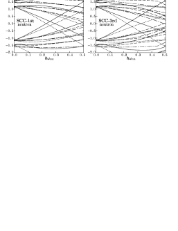
Fig. 6: Neutron quasiparticle Routhians plotted as functions of $\hbar\mathchar 28961\relax_{\rm rot}$ (MeV) suitable for ¹⁶²Er. They are obtained by diagonalizing the SCC quasiparticle Hamiltonian (3.48) up to the first order (left) and third order (right) of the $\mathchar 28961\relax$-expansion. As in the case of the usual adiabatic quasiparticle energy diagram, the negative energy solutions, $-E^{\prime}_{\mathchar 28950\relax}=E^{\prime}_{\bar{\mathchar 28950\relax}}$ and $-E^{\prime}_{\bar{\mathchar 28951\relax}}=E^{\prime}_{\mathchar 28951\relax}$, are also drawn. The solid, dotted, dashed, and dash-dotted curves denote Routhians with $(\mathchar 28953\relax,r)=(+,+i)$, $(+,-i)$, $(-,+i)$, and $(-,-i)$, respectively.

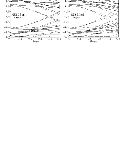
Fig. 7: Same as Fig. 6 but for proton quasiparticles.

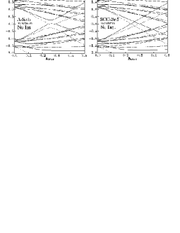
Fig. 8: Same as Fig. 6 but obtained by the adiabatic cranking (left) and the third order SCC (right) with neglecting the residual interactions.

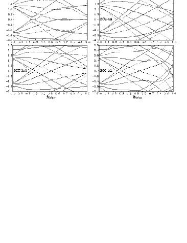
Fig. 9: Neutron quasiparticle Routhians for the $N_{\rm osc}=6$ ($i_{13/2}$) orbits suitable for ¹⁶²Er. The left upper, right upper, left lower, and right lower panels denote the results of the adiabatic cranking, the SCC up to the first order, 3rd order, and 5th order, respectively. The solid and dotted curves denote Routhians with $r=+i$ $(\mathchar 28939\relax=-1/2)$ and $r=-i$ $(\mathchar 28939\relax=+1/2)$, respectively. The effect of residual interaction is completely neglected in this calculation.

Now let us study the quasiparicle Routhians obtained by means of the SCC method. It is mentioned in §3.2 that the two step diagonalization with the truncation of the $\mathchar 28961\relax$-expansion up to ${n_{\rm max}}$, c.f. Eq. (3.48), leads to diabatic quasiparticle states in the rotating frame, in which the negative and positive eigenstates do not interact with each other. We show in Figs. 6 and 7 calculated quasiparticle Routhians for neutrons and protons, respectively. It is confirmed that the diabatic quasiparticle states are obtained. As discussed in §3.2, the diagonalization of the quasiparticle Hamiltonian in the SCC method is completely equivalent to that of the selfconsistent cranking model, which is known to lead to the adiabatic levels, if the first step unitary transformation $e^{iG(\mathchar 28961\relax)}$ is treated non-perturbatively in full order. Then what is the mechanism that realizes the diabatic levels? We believe that the cutoff of the $\mathchar 28961\relax$-expansion extracts the smoothly varying part of the quasiparticle Hamiltonian; namely, ignoring its higher order terms eliminates the cause of abrupt changes of the microscopic internal structure by quasiparticle alignments. An analogous mechanism has been known for many years in the Strutinsky smoothing procedure:[14]  The $\mathchar 28942\relax$-function in the microscopic level density is replaced by the Gaussian smearing function times the sum of the Hermite polynomials (complete set), and the lower order cutoff of the sum (usually 6th order is taken) gives the smoothed level density. It should be noted, however, that the plateau condition guarantees that the order of cutoff does not affect the physical results in the case of the Strutinsky method. We have not yet succeeded in obtaining such a condition in the present case of the cutoff of the $\mathchar 28961\relax$-expansion in the SCC method for the collective rotation. Therefore we have to decide the ${n_{\rm max}}$ value by comparison of the calculated results with experimental data. We mainly take ${n_{\rm max}}=3$ in the following; determination of the optimal choice of ${n_{\rm max}}$ remains as a future problem.

In Figs. 6 and 7 the results obtained by truncating up to the first order (${n_{\rm max}}=1$) and the third order (${n_{\rm max}}=3$) are compared. It is clear that the higher order terms considerably modify the quasiparticle energy diagrams. Especially, the alignments of the lowest pair of quasiparticles are reduced for neutrons (low $K$ states of the $i_{13/2}$-orbitals), while they are increased for protons (medium $K$ states of the $h_{11/2}$-orbitals). Thus, the higher order effects depend strongly on the nature of orbitals. It should be stressed that the effects of the residual interaction, i.e. changes of the mean-field against the collective rotation, are contained in the quasiparticle diagrams presented in these figures. In this sense, they are different from the spectra of the cranked shell model,[40]  where the mean-field is fixed at $\mathchar 28961\relax=0$. In Fig. 8 are displayed the usual adiabatic quasineutron Routhians and the third order SCC Routhians, in both of which the residual interactions are neglected completely. Again, by comparing Fig. 8 with Fig. 6, it is seen that the effect of residual interactions considerably changes the quasiparticle states. In relation to the choice of ${n_{\rm max}}$, we compare in Fig. 9 the Routhians obtained by changing the cutoff order ${n_{\rm max}}=1,3,5$. In this figure, the usual non-selfconsistent adiabatic Routhians are also displayed, and for comparison’s sake, the residual interactions are completely neglected in all cases. Moreover, the rotational frequency is extended to unrealistically large values in order to see the asymptotic behaviors of the Routhian. Comparing the adiabatic Routhians with those of the SCC method, positive and negative energy solutions cross irrespective of the strength of level-repulsion. Although the adiabatic levels change their characters abruptly at the crossing, if their average behaviors are compared to the calculated ones, the third order results (${n_{\rm max}}=3$) agree best with the adiabatic levels. The first order results, for example, give the alignments (the slopes of Routhians) too large. On the other hand, the divergent behaviors are clearly seen at about $\mathchar 28961\relax\geq 0.8$ MeV in the fifth order results. The inclusion of the effect of the residual interactions makes this convergence radius in $\mathchar 28961\relax$ even smaller.

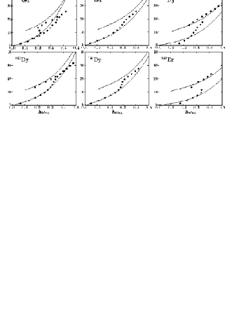
Fig. 10: Comparison of the third order SCC method calculations for the diabatic $g$- and $s$-bands with experimental data. The angular momenta $\langle J_{x}\rangle=I+1/2$ ($\hbar$) are displayed versus the rotational frequency $\hbar\mathchar 28961\relax_{\rm rot}$ (MeV) for nuclei in the rare-earth region, Gd ($Z=64$) to W ($Z=74$) isotopes. Filled circles denote experimental data smoothly extended from the ground state. Data for excited bands are also included as filled squares when available, which are, in most cases, identified as $s$-bands.

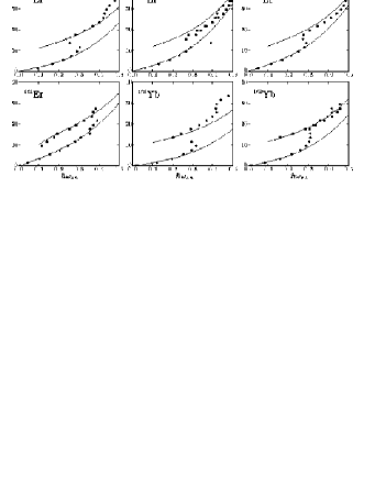
Fig. 10: continued.

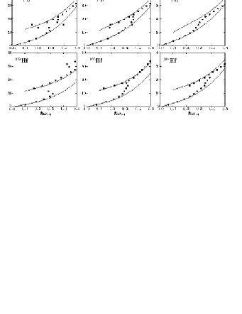
Fig. 10: continued.

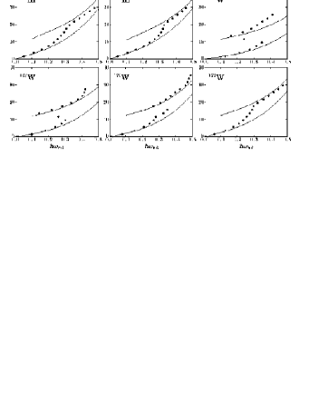
Fig. 10: continued.

Finally, we would like to discuss the results of application of the present formalism to the $g$- and $s$-bands, which are observed systematically and compose the yrast lines of even-even nuclei. Although we can compare the Routhians (3.21), or equivalently the rotational energy (3.13), it is known that the relation $I_{x}$ versus $\mathchar 28961\relax$ gives a more stringent test. Therefore we compare the calculated $I_{x}-\mathchar 28961\relax$ relation with the experimental one in Fig. 10 for even-even nuclei in the rare-earth region, in which the band crossings are identified along the yrast sequences. In this calculation the $I_{x}(\mathchar 28961\relax)$ of the $g$-band is given by Eq. (3.82) with calculated values of the Harris parameters (see Table II). As for the $I_{x}(\mathchar 28961\relax)$ of the $s$-band, we calculate it on the simplest assumption of the independent quasiparticle motions in the rotating frame, which is the same as that of the cranked shell model:

$$|\mathchar 28958\relax_{s}(\mathchar 28961\relax)\rangle=\mathchar 28939\relax^{\dagger}_{1}(\mathchar 28961\relax)\mathchar 28939\relax^{\dagger}_{\bar{1}}(\mathchar 28961\relax)|\mathchar 28958\relax_{\rm intr}(\mathchar 28961\relax)\rangle,\quad|\mathchar 28958\relax_{g}(\mathchar 28961\relax)\rangle=|\mathchar 28958\relax_{\rm intr}(\mathchar 28961\relax)\rangle,$$ (3.89)

where $\mathchar 28939\relax^{\dagger}_{1}(\mathchar 28961\relax)$ and $\mathchar 28939\relax^{\dagger}_{\bar{1}}(\mathchar 28961\relax)$ are the lowest $r=+i$ and $r=-i$ quasineutron creation operators in the rotating frame. Then, the $I_{x}(\mathchar 28961\relax)$ of the $s$-band is the sum of $I_{x}(\mathchar 28961\relax)$ of the $g$-band and the aligned angular momenta of two quasineutrons, which are calculated according to Eqs. (3.51)$-$(3.54),

$$\bigl{(}I_{x}(\mathchar 28961\relax)\bigr{)}_{s\hbox{-}{\rm band}}=I_{x}(\mathchar 28961\relax)+i_{1}(\mathchar 28961\relax)+i_{\bar{1}}(\mathchar 28961\relax),\quad\bigl{(}I_{x}(\mathchar 28961\relax)\bigr{)}_{g\hbox{-}{\rm band}}=I_{x}(\mathchar 28961\relax),$$ (3.90)

or by using the canonical relation between the Routhian and the aligned angular momentum, the alignments $i_{\mathchar 28950\relax}$ and $i_{\bar{\mathchar 28950\relax}}$ can be calculated as usual:

$$i_{\mathchar 28950\relax}(\mathchar 28961\relax)=-{\partial E^{\prime}_{\mathchar 28950\relax}(\mathchar 28961\relax)\over\partial\mathchar 28961\relax},\quad i_{\bar{\mathchar 28950\relax}}(\mathchar 28961\relax)=-{\partial E^{\prime}_{\bar{\mathchar 28950\relax}}(\mathchar 28961\relax)\over\partial\mathchar 28961\relax}.$$ (3.91)

Since our quasiparticle Routhians behave diabatically as functions of the rotational frequency, the resultant $g$- and $s$-bands are also non-interacting bands; we have to mix them at the same angular momentum to obtain the interacting bands corresponding to the observed bands. Such a band mixing calculation is straightforward in our formalism if the interband $g$-$s$ interaction is provided. However, it is a very difficult task as long as the usual adiabatic cranking model is used. In the present stage we are not able to estimate the $g$-$s$ interband interaction theoretically. Therefore, we do not attempt to perform such band-mixing calculations in the present paper (but see §4.2).

Looking into the results displayed in Fig. 10, one see that our diabatic formalism of collective rotation based on the SCC method is quite successful. The overall agreements are surprisingly good, considering the fact that we have only used a global parametrization of the strengths of the residual interaction:

$$G_{0}^{\mathchar 28951\relax}=20/A,\quad G_{0}^{\mathchar 28953\relax}=24/A\;\;{\rm(MeV)},$$ (3.92)

$$g_{2}^{\mathchar 28951\relax}=g_{2}^{\mathchar 28953\relax}=24,$$ (3.93)

$$\mathchar 28948\relax_{2K}=1.45\,\mathchar 28948\relax_{2}^{\rm self},$$ (3.94)

for the model space of three $N_{\rm osc}$-shells ($4-6$ for neutrons and $3-5$ for protons). The agreements of the calculated $g$-bands come from the fact that the Harris parameters (Table II) are nicely reproduced in the calculation. Further agreements of the $s$-bands are not trivial, and tell us that we have obtained reliable diabatic quasiparticle spectra (Figs. 6 and 7). It is known that, if the $I_{x}-\mathchar 28961\relax$ relations of $s$-bands are parametrized in the form, $I_{x}=i+{\cal J}_{0}\,\mathchar 28961\relax+{\cal J}_{1}\,\mathchar 28961\relax^{3}$, the ${\cal J}_{1}$ Harris parameters of $s$-bands are systematically smaller than those of $g$-bands. This feature is quite well reproduced in the calculations, as is clearly seen in Fig. 10, and the reason is that the value of the aligned angular momentum of two quasineutrons decreases as a function of $\mathchar 28961\relax$. The suitable decrease is obtainable only if the residual interactions are included and the diabatic quasiparticle Routhians are evaluated up to the third order.

4 Diabatic quasiparticle basis and the interband interaction between the $g$- and $s$-bands

The formulation of the previous section gives a consistent perturbative solution, with respect to the rotational frequency, of the basic equations of the SCC method for collective rotation. However, it has a problem as a method to construct the diabatic quasiparticle basis: The wave functions of the diabatic levels are orthonormal only within the order of cutoff (${n_{\rm max}}$) of the $\mathchar 28961\relax$-expansion. In the previous section only the independent quasiparticle states, i.e. one-quasiparticle states or the $g$- and $s$-bands, are considered and this problem does not show up. The quasiparticle states have another important role that they are used as a basis of complete set for a more sophisticated many body technique beyond the mean-field approximation; for example, the study of collective vibrations at high spin in terms of the RPA method in the rotating frame.[7, 52, 57, 58, 59, 60]  In such an application it is crucial that the diabatic quasiparticle basis satisfies the orthonormal property. We present in this section a possible method to construct the diabatic basis satisfying the orthonormality condition.

Another remaining problem which is not touched in the previous section is how to theoretically evaluate the interband interaction between the ground state band and the two quasineutron aligned band. Since we do not have satisfactory answer yet to this problem, we only present a scope for possible solutions at the end of this section.

4.1 Construction of diabatic quasiparticle basis in the SCC method

Although the basic idea is general, we restrict ourselves to the case of collective rotation and use the good signature representation with real phase convention, introduced in §3.3, for the matrix elements of the Hamiltonian $H$ and of the angular momentum $J_{x}$. First let us recall that the diabatic quasiparticle basis in the rotating frame is obtained by the two step unitary transformation (3.45). The first transformation by $e^{iG(\mathchar 28961\relax)}$ can be represented as follows,[10]

$$e^{iG(\mathchar 28961\relax)}a^{\dagger}_{i}e^{-iG(\mathchar 28961\relax)} = \sum_{j>0}\bigl{[}\cos{\sqrt{gg^{\rm T}}}\bigr{]}_{ij}a^{\dagger}_{j}-\sum_{j>0}\Bigl{[}g\,{\displaystyle{\sin{\sqrt{g^{\rm T}g}}\over\sqrt{g^{\rm T}g}}}\Bigr{]}_{ij}a_{\bar{j}},$$ (4.1)

$$e^{iG(\mathchar 28961\relax)}a^{\dagger}_{\bar{i}}e^{-iG(\mathchar 28961\relax)} = \sum_{j>0}\bigl{[}\cos{\sqrt{g^{\rm T}g}}\bigr{]}_{ij}a^{\dagger}_{\bar{j}}+\sum_{j>0}\Bigl{[}g^{\rm T}\,{\displaystyle{\sin{\sqrt{gg^{\rm T}}}\over\sqrt{gg^{\rm T}}}}\Bigr{]}_{ij}a_{j},$$ (4.2)

with real matrix elements $g_{ij}(\mathchar 28961\relax)=\sum_{n\geq 1}\mathchar 28961\relax^{n}g^{(n)}(ij)$, see Eq. (3.64), where $g^{\rm T}$ denotes the transpose of $g$. Thus, by using an obvious matrix notation, the transformation to the rotating quasiparticle operator from the $\mathchar 28961\relax=0$ quasiparticle operator is given as

$$\left(\begin{array}[]{l}\mathchar 28939\relax\\ {\bar{\mathchar 28939\relax}}^{\dagger}\end{array}\right) = \left(\begin{array}[]{cc}f^{\rm T}&0\\ 0&{\bar{f}}^{\,{\rm T}}\end{array}\right)\left(\begin{array}[]{cc}\cos{\sqrt{gg^{\rm T}}}&-g\,{\displaystyle{\sin{\sqrt{g^{\rm T}g}}\over\sqrt{g^{\rm T}g}}}\\ g^{\rm T}\,{\displaystyle{\sin{\sqrt{gg^{\rm T}}}\over\sqrt{gg^{\rm T}}}}&\cos{\sqrt{g^{\rm T}g}}\end{array}\right)\left(\begin{array}[]{l}a\\ {\bar{a}}^{\dagger}\end{array}\right)$$ (4.11)

$$\equiv {\cal F}^{\rm T}(\mathchar 28961\relax)\,{\cal G}^{\rm T}(\mathchar 28961\relax)\left(\begin{array}[]{l}a\\ {\bar{a}}^{\dagger}\end{array}\right),$$ (4.14)

where the real matrix elements $f_{i\mathchar 28950\relax}(\mathchar 28961\relax)$ and ${\bar{f}}_{i\mathchar 28950\relax}(\mathchar 28961\relax)$ are the amplitudes that diagonalize the quasiparticle Hamiltonian in the rotating frame, see Eq. (3.42), for signature $r=+i$ and $-i$, respectively. The cutoff of the $\mathchar 28961\relax$-expansion means that the generator $iG(\mathchar 28961\relax)$, i.e. the matrix $g$, is solved up to the $n={n_{\rm max}}$ order,

$$g(\mathchar 28961\relax)=[g(\mathchar 28961\relax)]^{(n\leq{n_{\rm max}})}=\sum_{n=1}^{n_{\rm max}}\mathchar 28961\relax^{n}g^{(n)},$$ (4.15)

and at the same time the transformation matrix ${\cal G}(\mathchar 28961\relax)$ itself is treated perturbatively

$${\cal G}(\mathchar 28961\relax)=\left(\begin{array}[]{cc}1-\mathchar 28961\relax^{2}g^{(1)}g^{(1){\rm T}}+\cdots&\mathchar 28961\relax g^{(1)}+\cdots\\ -\mathchar 28961\relax g^{(1){\rm T}}+\cdots&1-\mathchar 28961\relax^{2}g^{(1){\rm T}}g^{(1)}+\cdots\end{array}\right),$$ (4.16)

while the other one, ${\cal F}(\mathchar 28961\relax)$, is treated non-perturbatively by the diagonalization procedure. The origin of difficulty arising when the diabatic basis is utilized as a complete set lies in this treatment of ${\cal G}(\mathchar 28961\relax)$, because the orthogonality of the matrix ${\cal G}(\mathchar 28961\relax)$ is broken in higher-orders.

Now the solution to this problem is apparent: The generator matrix $g(\mathchar 28961\relax)$ is solved perturbatively like in Eq.(4.15), but the transformation matrix ${\cal G}(\mathchar 28961\relax)$ has to be treated non-perturbatively as in Eq. (4.11). In order to realize this treatment we introduce new orthogonal matrices, $D$ and ${\bar{D}}$, which diagonalize $gg^{\rm T}$ and $g^{\rm T}g$ within the signature $r=+i$ and $-i$ states, respectively,

$$\sum_{j>0}(gg^{\rm T})_{ij}D_{jk}=D_{ik}\mathchar 28946\relax^{2}_{k},\quad\sum_{j>0}(g^{\rm T}g)_{ij}{\bar{D}}_{jk}={\bar{D}}_{ik}\mathchar 28946\relax^{2}_{k},$$ (4.17)

where we have used the fact that the matrices $gg^{\rm T}$ and $g^{\rm T}g$ have common eigenvalues, which are non-negative, and then we have

$${\cal G}(\mathchar 28961\relax)=\left(\begin{array}[]{cc}D(\cos{\mathchar 28946\relax})D^{\rm T}&g{\bar{D}}(\sin{\mathchar 28946\relax}/\mathchar 28946\relax){\bar{D}}^{\rm T}\\ -g^{\rm T}D(\sin{\mathchar 28946\relax}/\mathchar 28946\relax)D^{\rm T}&{\bar{D}}(\cos{\mathchar 28946\relax}){\bar{D}}^{\rm T}\end{array}\right).$$ (4.20)

Here ($\cos{\mathchar 28946\relax}$) and ($\sin{\mathchar 28946\relax}/\mathchar 28946\relax$) denote diagonal matrices, whose matrix elements are $\mathchar 28942\relax_{ij}\cos{\mathchar 28946\relax_{i}}$ and $\mathchar 28942\relax_{ij}\sin{\mathchar 28946\relax_{i}}/\mathchar 28946\relax_{i}$, respectively. The physical meaning is that the orthogonal matrices $D$ and ${\bar{D}}$ are transformation matrices from the quasiparticle operators $(a^{\dagger}_{i},a_{i})$ and $(a^{\dagger}_{\bar{i}},a_{\bar{i}})$ at $\mathchar 28961\relax=0$ to their canonical bases, which diagonalize the density matrices $\mathchar 28954\relax$ and ${\bar{\mathchar 28954\relax}}$ with respect to the rotational HB state $|\mathchar 28958\relax_{\rm intr}(\mathchar 28961\relax)\rangle$, respectively;

$$\mathchar 28954\relax_{ij} \equiv \langle\mathchar 28958\relax_{\rm intr}(\mathchar 28961\relax)|a^{\dagger}_{i}a_{j}|\mathchar 28958\relax_{\rm intr}(\mathchar 28961\relax)\rangle=\bigl{[}\cos{\sqrt{gg^{\rm T}}}\bigr{]}_{ij},$$

$${\bar{\mathchar 28954\relax}}_{ij} \equiv \langle\mathchar 28958\relax_{\rm intr}(\mathchar 28961\relax)|a^{\dagger}_{\bar{i}}a_{\bar{j}}|\mathchar 28958\relax_{\rm intr}(\mathchar 28961\relax)\rangle=\bigl{[}\cos{\sqrt{g^{\rm T}g}}\bigr{]}_{ij}.$$ (4.21)

Thus the method to construct the rotating quasiparticle basis is summarized as follows. First, solve the basic equation of the SCC method and obtain the generator matrix $g(\mathchar 28961\relax)$ up to the ${n_{\rm max}}$ order as in Eq. (4.15). At the same time, diagonalize the quasiparticle Hamiltonian and obtain the eigenstates as in Eq. (3.42) for both signatures $r=\pm i$. Secondly, diagonalize the density matrices (4.21), or equivalently Eq. (4.17), and obtain the orthogonal matrices $D$ and ${\bar{D}}$ of the canonical bases. Finally, by using these matrices $D$ and ${\bar{D}}$ calculate the transformation matrix ${\cal G}(\mathchar 28961\relax)$ as in Eq. (4.20), and then the basis transformation is determined by Eq. (4.14).

It is instructive to consider a concrete case of the cranked shell model; i.e. the effect of residual interactions or the selfconsistency of mean-field is neglected at $\mathchar 28961\relax>0$. The quasiparticle basis is obtained by diagonalizing the generalized Hamiltonian matrix:

$$\left(\begin{array}[]{cc}h_{\rm Nils}-\mathchar 28961\relax j_{x}&-\mathchar 28929\relax\\ -\mathchar 28929\relax&-(h_{\rm Nils}+\mathchar 28961\relax j_{x})\end{array}\right)\left(\begin{array}[]{cc}U&{\bar{V}}\\ V&{\bar{U}}\end{array}\right)=\left(\begin{array}[]{cc}U&{\bar{V}}\\ V&{\bar{U}}\end{array}\right)\left(\begin{array}[]{cc}E^{\prime}&0\\ 0&-{\bar{E}}^{\prime}\end{array}\right),$$ (4.22)

where $h_{\rm Nils}$ and $j_{x}$ denote matrices with respect to the Nilsson (or the harmonic oscillator) basis at $\mathchar 28961\relax=0$, and $(U,V)$ and $({\bar{U}},{\bar{V}})$ are coefficients of the generalized Bogoliubov transformations from the Nilsson nucleon operators $(c^{\dagger}_{i},c_{i})$ and $(c^{\dagger}_{\bar{i}},c_{\bar{i}})$ (in the good signature representation),

$$\mathchar 28939\relax^{\dagger}_{\mathchar 28950\relax}=\sum_{i>0}(U_{i\mathchar 28950\relax}c^{\dagger}_{i}+V_{i\mathchar 28950\relax}c_{\bar{i}}),\quad\mathchar 28939\relax^{\dagger}_{\bar{\mathchar 28950\relax}}=\sum_{i>0}({\bar{U}}_{i\mathchar 28950\relax}c^{\dagger}_{\bar{i}}+{\bar{V}}_{i\mathchar 28950\relax}c_{i}),$$ (4.23)

or in the matrix notation

$$\left(\begin{array}[]{l}c\\ {\bar{c}}^{\dagger}\end{array}\right)={\cal U}\left(\begin{array}[]{l}\mathchar 28939\relax\\ {\bar{\mathchar 28939\relax}}^{\dagger}\end{array}\right),\quad{\cal U}\equiv\left(\begin{array}[]{cc}U&{\bar{V}}\\ V&{\bar{U}}\end{array}\right).$$ (4.24)

In contrast, the transformation ${\cal U}$ is decomposed into three steps in our construction method of the diabatic quasiparticle basis; (i) the Bogoliubov transformation ${\cal U}_{0}$ between the nucleon $(c,{\bar{c}}^{\dagger})$ and the quasiparticle $(a,{\bar{a}}^{\dagger})$ at $\mathchar 28961\relax=0$,

$$\left(\begin{array}[]{l}c\\ {\bar{c}}^{\dagger}\end{array}\right)={\cal U}_{0}\left(\begin{array}[]{l}a\\ {\bar{a}}^{\dagger}\end{array}\right),\quad{\cal U}_{0}\equiv\left(\begin{array}[]{cc}u&v\\ -v^{\rm T}&u\end{array}\right),$$ (4.25)

where $u$ and $v$ are the matrices of transformation at $\mathchar 28961\relax=0$, (they are diagonal, e.g. $u_{ij}=u_{i}\mathchar 28942\relax_{ij}$, if only the monopole-pairing interaction is included), (ii) the transformation matrix ${\cal G}(\mathchar 28961\relax)$ in Eq. (4.14), generated by $e^{iG(\mathchar 28961\relax)}$, and (iii) the diagonalization step of the rotating quasiparticle Hamiltonian ${\cal F}(\mathchar 28961\relax)$ in Eq. (4.14), see also Eq. (3.42), namely

$${\cal U}(\mathchar 28961\relax)^{\rm SCC}={\cal U}_{0}\,{\cal G}(\mathchar 28961\relax){\cal F}(\mathchar 28961\relax).$$ (4.26)

Here both ${\cal G}(\mathchar 28961\relax)$ and ${\cal F}(\mathchar 28961\relax)$ depend on the order of cutoff ${n_{\rm max}}$ in solving the generator $iG(\mathchar 28961\relax)$ by the $\mathchar 28961\relax$-expansion method, but they themselves have to be calculated non-perturbatively, especially for ${\cal G}$ by Eq. (4.20) with (4.17). As noticed in the end of §3.3, we can apply the SCC method starting from the finite frequency $\mathchar 28961\relax_{0}$. In such a case ${\cal U}_{0}$ is the transformation at $\mathchar 28961\relax=\mathchar 28961\relax_{0}$, and ${\cal G}$ and ${\cal F}$ are obtained by expansions in terms of $(\mathchar 28961\relax-\mathchar 28961\relax_{0})$; thus,

$${\cal U}(\mathchar 28961\relax)^{\rm SCC}={\cal U}_{0}(\mathchar 28961\relax_{0})\,{\cal G}(\mathchar 28961\relax-\mathchar 28961\relax_{0}){\cal F}(\mathchar 28961\relax-\mathchar 28961\relax_{0})\quad{\rm if\;started\;at\;}\mathchar 28961\relax=\mathchar 28961\relax_{0}.$$ (4.27)

It should be stressed that the transformation (4.26) only approximately diagonalize the Hamiltonian in Eq. (4.22) within the ${n_{\rm max}}$ order in the sense of $\mathchar 28961\relax$-expansion. Namely, some parts of the Hamiltonian corresponding to the terms higher order than ${n_{\rm max}}$ are neglected, and this is exactly the reason why we can obtain the diabatic basis, whose negative and positive solutions are non-interacting.

In the case where the effect of residual interactions is neglected, i.e. corresponding to the higher order cranking, we can easily solve the basic equations of the SCC method. It is useful to present the solution for practical purposes; for example for the construction of the diabatic quasiparticle basis for the cranked shell model calculations. The solutions for $g^{(n)}$ up to the third order are given as follows:

$$g^{(1)}(ij) = {1\over E_{i}+E_{\bar{j}}}J_{x}^{A}(ij),$$ (4.28)

$$g^{(2)}(ij) = {1\over E_{i}+E_{\bar{j}}}(J_{x}^{B}g^{(1)}+g^{(1)}{\bar{J}}_{x}^{B})_{ij},$$ (4.29)

$$g^{(3)}(ij) = {1\over E_{i}+E_{\bar{j}}}\bigl{[}(J_{x}^{B}g^{(2)}+g^{(2)}{\bar{J}}_{x}^{B})$$ (4.30)

$$\quad+{1\over 3}(J_{x}^{A}g^{(1){\rm T}}g^{(1)}+2g^{(1)}J_{x}^{A{\rm T}}g^{(1)}+g^{(1)}g^{(1){\rm T}}J_{x}^{A})\bigr{]}_{ij},$$

and the solutions for the rotating quasiparticle Hamiltonian (3.48)$-$(3.49):

$$\mathchar 28943\relax^{\prime(0)}_{ij} = \mathchar 28942\relax_{ij}E_{i},\quad{\bar{\mathchar 28943\relax}}^{\prime(0)}_{ij}=\mathchar 28942\relax_{ij}E_{\bar{i}},$$ (4.31)

$$\mathchar 28943\relax^{\prime(1)}_{ij} = -J_{x}^{B}(ij),\quad{\bar{\mathchar 28943\relax}}^{\prime(1)}_{ij}=-{\bar{J}}_{x}^{B}(ij),$$ (4.32)

$$\mathchar 28943\relax^{\prime(2)}_{ij} = {1\over 2}(J_{x}^{A}g^{(1){\rm T}}+g^{(1)}J_{x}^{A{\rm T}})_{ij},\quad{\bar{\mathchar 28943\relax}}^{\prime(2)}_{ij}={1\over 2}(J_{x}^{A{\rm T}}g^{(1)}+g^{(1){\rm T}}J_{x}^{A})_{ij},$$ (4.33)

$$\mathchar 28943\relax^{\prime(3)}_{ij} = {1\over 2}(J_{x}^{A}g^{(2){\rm T}}+g^{(2)}J_{x}^{A{\rm T}})_{ij},\quad{\bar{\mathchar 28943\relax}}^{\prime(3)}_{ij}={1\over 2}(J_{x}^{A{\rm T}}g^{(2)}+g^{(2){\rm T}}J_{x}^{A})_{ij},$$ (4.34)

where the quasiparticle energies at the starting frequency are given in Eq. (3.62), and the matrix elements of $J_{x}$ at the starting frequency are given as in Eq. (3.63) with $Q_{\mathchar 28954\relax}$ replaced by $J_{x}$. If the starting frequency is $\mathchar 28961\relax=0$, then $E_{\bar{i}}=E_{i}$, and the matrix elements of $J_{x}$ satisfy the relations, $J_{x}^{A{\rm T}}=-J_{x}^{A}$, ${\bar{J}}_{x}^{B}=-J_{x}^{B}$, and $J_{x}^{B{\rm T}}=J_{x}^{B}$. The transformation ${\cal G}(\mathchar 28961\relax)$ is calculated from Eqs. (4.28)$-$(4.30), and ${\cal F}(\mathchar 28961\relax)$ from Eqs. (4.31)$-$(4.34). It should be mentioned that the selfconsistent mean-field calculation is in principle possible in combination with the diabatic basis prescription presented above.

4.2 Estimate of the $g$-$s$ interaction

Once the diabatic $g$- and $s$-bands states (3.89) are obtained as functions of $\mathchar 28961\relax$, one can immediately construct them as functions of angular momentum $I$, because the $I_{x}-\mathchar 28961\relax$ relation has no singularity, as shown in Fig. 10, and can easily be inverted:

$$|\mathchar 28958\relax_{g}(I)\rangle=|\mathchar 28958\relax_{g}(\mathchar 28961\relax_{g}(I))\rangle,\quad|\mathchar 28958\relax_{s}(I)\rangle=|\mathchar 28958\relax_{s}(\mathchar 28961\relax_{s}(I))\rangle,$$ (4.35)

where $\mathchar 28961\relax_{g}(I)$ and $\mathchar 28961\relax_{s}(I)$ are the inverted relations of (3.90) with $I_{x}=I+1/2$. Physically, one has to consider the coupling problem between them at a fixed spin value $I$. It is, however, a difficult problem because one has to calculate, for example, a matrix element like $\langle\mathchar 28958\relax_{s}(I)|H|\mathchar 28958\relax_{g}(I)\rangle$, which is an overlap between two different HB states; they are not orthogonal to each other due to the difference of the frequencies $\mathchar 28961\relax_{g}(I)$ and $\mathchar 28961\relax_{s}(I)$. Although such a calculation is possible by using the Onishi formula for the overlap of general HB states,[35]  it would damage the simple picture of quasiparticle motions in the rotating frame, and is out of scope of the present investigation.

Here we assume that the wave functions varies smoothly along the diabatic rotational bands as functions of spin $I$ or frequency $\mathchar 28961\relax$, so that the interband interaction between the $g$- and $s$-bands can be evaluated at the common frequency by

$$v_{g\mbox{-}s}(I)=\langle\mathchar 28958\relax_{s}(\mathchar 28961\relax_{gs}(I))|H|\mathchar 28958\relax_{g}(\mathchar 28961\relax_{gs}(I))\rangle,$$ (4.36)

where $\mathchar 28961\relax_{gs}$ is defined by an average of $\mathchar 28961\relax_{s}$ and $\mathchar 28961\relax_{g}$,

$$\mathchar 28961\relax_{gs}(I)\equiv{\mathchar 28961\relax_{g}(I)+\mathchar 28961\relax_{s}(I)\over 2}.$$ (4.37)

We note that this quantity corresponds, in a good approximation, to the crossing frequency $\mathchar 28961\relax_{\rm c}^{g\mbox{-}s}$ at the crossing angular momentum $I_{\rm c}^{g\mbox{-}s}$,

$$\mathchar 28961\relax_{gs}(I_{\rm c}^{g\mbox{-}s})\approx\mathchar 28961\relax_{\rm c}^{g\mbox{-}s},$$ (4.38)

where $\mathchar 28961\relax_{\rm c}^{g\mbox{-}s}$ is defined as a frequency at which the lowest diabatic two quasiparticle energy vanishes, $E^{\prime}_{1}(\mathchar 28961\relax)+E^{\prime}_{\bar{1}}(\mathchar 28961\relax)=0$. Using the fact that $|\mathchar 28958\relax_{s}(\mathchar 28961\relax)\rangle$ is the two quasiparticle excited state on $|\mathchar 28958\relax_{g}(\mathchar 28961\relax)\rangle$ (see Eq. (3.89)), the interaction can be rewritten as

$$v_{g\mbox{-}s}(I)=\mathchar 28961\relax_{gs}(I)\langle\mathchar 28958\relax_{s}(\mathchar 28961\relax_{gs}(I))|J_{x}|\mathchar 28958\relax_{g}(\mathchar 28961\relax_{gs}(I))\rangle,$$ (4.39)

because of the variational principle (3.19). Applying the idea of $\mathchar 28961\relax$-expansion and taking up to the lowest order, we have, at the crossing angular momentum $I_{\rm c}^{g\mbox{-}s}$,

$$v_{g\mbox{-}s}(I_{\rm c}^{g\mbox{-}s})\approx\mathchar 28961\relax_{\rm c}^{g\mbox{-}s}\sum_{ij>0}f_{i1}(\mathchar 28961\relax_{\rm c}^{g\mbox{-}s}){\bar{f}}_{j1}(\mathchar 28961\relax_{\rm c}^{g\mbox{-}s})J_{x}^{A}(ij),$$ (4.40)

where $f_{i1}(\mathchar 28961\relax)$ and ${\bar{f}}_{j1}(\mathchar 28961\relax)$ are the amplitudes of the diabatic quasiparticle diagonalization (3.42) for the lowest $r=\pm i$ quasineutrons, and should be calculated non-perturbatively with respect to $\mathchar 28961\relax$.

In Fig. 11 (right panel), we show the result evaluated by using Eq. (4.40) for a simple single-$j$ shell model ($i_{13/2}$) with a constant monopole-pairing gap and no residual interactions, in which the single-particle energies are given by

$$e_{i}=\mathchar 28948\relax\,{3m_{i}^{2}-j(j+1)\over j(j+1)}\quad(m_{i}=1/2,\cdots,j),$$ (4.41)

with a parameter $\mathchar 28948\relax$ describing the nuclear deformation. In this figure other quantities, the alignment of the lowest two quasiparticle state, the number expectation value, and the crossing frequency are also shown as functions of the chemical potential. These quantities can also be evaluated in terms of the usual adiabatic cranking model, and they are also displayed in the left panel. Note that in the adiabatic cranking model the crossing frequency is defined as a frequency at which the adiabatic two quasiparticle energy $E^{\prime({\rm ad})}_{1}(\mathchar 28961\relax)+E^{\prime({\rm ad})}_{\bar{1}}(\mathchar 28961\relax)$ becomes the minimum, and the interband interaction is identified as the half of its minimum value.[40]  As is well known,[61]  the $g$-$s$ interaction oscillates as a function of the chemical potential, and both the absolute values and the oscillating behavior of the result of calculation roughly agree with the experimental findings. Comparing two calculations, the interband interaction (4.40) seems to give a possible microscopic estimate based on the diabatic description of the $g$- and $s$-bands. We would like to stress, however, that its derivation is not very sound. It is an important future problem to derive the coupling matrix element on a more sound ground.

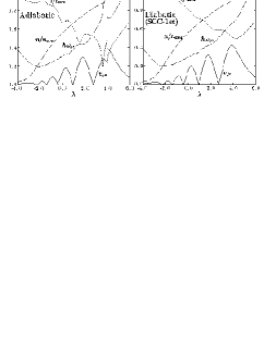
Fig. 11: The $g$-$s$ interband interaction (solid), the crossing frequency $\hbar\mathchar 28961\relax_{gs}$ (dash-dotted) in MeV, the alignment $i$ (dotted), and the expectation value of number operator $n$ (dashed), plotted as functions of the chemical potential $\mathchar 28949\relax$ in MeV, for the $i_{13/2}$ single-$j$ shell model without residual interactions. The result of the usual adiabatic cranked shell model is displayed in the left panel, while that of the diabatic SCC 1st order calculation in the right panel. Here the alignment $i$ and the number $n$ is scaled by their maximum values, $i_{\rm max}=12\hbar$ and $n_{\rm max}=14$. The energy unit is chosen such that the splitting of the $i_{13/2}$-shell roughly reproduces that of a typical well deformed rare-earth nucleus; i.e. $\mathchar 28948\relax=2.5$ MeV in Eq. (4.41), and the constant $\mathchar 28929\relax=1.0$ MeV is used.

5 Concluding remarks

In this paper, we have formulated the SCC method for the nuclear collective rotation. By using the rotational frequency expansion rather than the angular momentum expansion, we have applied it to the description of the $g$- and $s$-bands successfully. The systematic calculation gives surprisingly good agreements with experimental data for both rotational bands. It has been demonstrated that the resultant quasiparticle states develop diabatically as functions of the rotational frequency; i.e. the negative and positive energy levels do not interact with each other. Although the formulation is mathematically equivalent to the selfconsistent cranking model, the cutoff of the $\mathchar 28961\relax$-expansion results in the diabatic levels and its mechanism is also discussed. The perturbative $\mathchar 28961\relax$-expansion is, however, inadequate to use the resultant quasiparticle basis states as a complete set. We have then presented a method to construct the diabatic quasiparticle basis set, which rigorously satisfies the orthonormality condition and can be safely used for the next step calculation, e.g. the RPA formalism for collective vibrations at high-spin.

In order to obtain a good overall description of the rotational band for nuclei in the rare-earth region, we have investigated the best possible form of residual quadrupole-pairing interactions. It is found that the double-stretched form factor is essential for reproducing the even-odd mass difference and the moment of inertia simultaneously.

Since the calculated $g$- and $s$-bands in our formulation are diabatic rotational bands, the interband interaction between them should be taken into account for their complete descriptions. As in any other mean-field model, however, the wave function obtained in our formalism is a wave packet with respect to the angular momentum variable. Therefore, it is not apparent how to evaluate the interband interaction from microscopic point of view. We have presented a possible estimate of the interaction, which leads to a value similar to that estimated by the level repulsion in the adiabatic cranking model. Further investigations are still necessary to give a definite conclusion to this problem.

References

- [1] I. Hamamoto, Treatise on Heavy-Ion Science, Vol. 3, ed. D. A. Bromly (Prenum Press, 1985), p. 313.
- [2] Z. Szymansky, Fast Nuclear Rotation, Clarendon Press, 1983.
- [3] I. Hamamoto, Nucl. Phys. A271 (1976), 15.
- [4] E. R. Marshalek and A. L. Goodman, Nucl. Phys. A294 (1978), 92.
- [5] R. Bengtsson and S. Frauendorf, Nucl. Phys. A314 (1979), 27.
- [6] S. Frauendorf, in Nuclear Physics, ed. C. H. Dasso, R. A. Broglia and A. Winther (North-Holland, 1982), p.111.
- [7] Y. R. Shimizu and K. Matsuyanagi, Prog. Theor. Phys. 70 (1983), 144; 72 (1984), 799.
- [8] T. Bengtsson, Nucl. Phys. A496 (1989), 56.
- [9] M. Matsuo, T. Døssing, E. Vigezzi, R. A. Broglia and K. Yoshida, Nucl. Phys. A617 (1997), 1.
- [10] T. Marumori, T. Maskawa, F. Sakata and A. Kuriyama, Prog. Theor. Phys. 64 (1980), 1294.
- [11] D. R. Bes and R. A. Sorensen, Advances in Nuclear Physics, Vol. 2, (Prenum Press, 1969), p.129.
- [12] S. G. Nilsson and O. Prior, Mat. Fys. Medd. Dan. Vid. Selsk. 32 (1961), no. 16.
- [13] D. Vautherin and D. M. Brink, Phys. Rev. C3 (1972), 626.
- [14] M. Brack, J. Damgaard, A. S. Jensen, H. C. Pauli, V. M. Strutinsky and C. Y. Wong, Rev. Mod. Phys. 44 (1972), 320.
- [15] I. Ragnarsson, S. G. Nilsson and R. K. Sheline, Phys. Rep. 45 (1978), 1.
- [16] S. G. Nilsson and I. Ragnarsson, Shapes and Shells in Nuclear Structure, Cambridge University Press, 1995.
- [17] H. Sakamoto and T. Kishimoto, Nucl. Phys. A501 (1989), 205; 242.
- [18] T. Kishimoto et al., Phys. Rev. Lett. 35 (1975), 552; T. Kishimoto, Proc. 1980 RCNP Int. Symp. Highly Exited States in Nuclear Reactions, Osaka, p.145.
- [19] E. R. Marshalek, Phys. Rev. 29 (1984), 640.
- [20] M. Baranger, K. Kumar, Nucl. Phys. A110 (1968), 490.
- [21] H. Sakamoto, Nucl. Phys. A557 (1993), 583c.
- [22] I. Hamamoto, Nucl. Phys. A232 (1974), 445.
- [23] M. Diebel, Nucl. Phys. A419 (1984), 353.
- [24] J. D. Garrett et al., Phys. Lett. B118 (1982), 297.
- [25] H. Sakamoto and T. Kishimoto, Phys. Lett. B245 (1990), 321.
- [26] T. Kubo, H. Sakamoto, T. Kammuri and T. Kishimoto, Phys. Rev. C54 (1996), 2331.
- [27] W. Satuła and R. Wyss, Phys. Rev. C50 (1994), 2888.
- [28] A. Bohr and B. R. Mottelson, Nuclear Structure, Vol. I, (W. A. Benjamin Inc., 1969).
- [29] A. Bohr and B. R. Mottelson, Nuclear Structure, Vol. II, (W. A. Benjamin Inc., 1975).
- [30] S. M. Harris, Phys. Rev. 138 (1965), B509.
- [31] T. Bengtsson and I. Ragnarsson, Nucl. Phys. A436 (1985) 14.
- [32] G. Audi and A. H. Wapstra, Nucl. Phys. A565 (1993), 1.
- [33] M. Sakai, Atomic and Nuclear Data Tables, 31 (1984), 399.
- [34] Evaluated Nuclear Structure Data File, http://isotopes.lbl.gov/isotopes/vuensdf.html.
- [35] P. Ring and P. Schuck, The Nuclear Many-Body Problem, (Springer-Verlag, 1980).
- [36] Y. R. Shimizu and K. Matsuyanagi, Prog. Theor. Phys. 74 (1985), 1346.
- [37] J. Terasaki, T. Marumori and F. Sakata, Prog. Theor. Phys. 85 (1991), 1235.
- [38] J. Terasaki, Prog. Theor. Phys. 88 (1992), 529.
- [39] J. Terasaki, Prog. Theor. Phys. 92 (1994), 535.
- [40] R. Bengtsson and S. Frauendorf, Nucl. Phys. A327 (1979), 139.
- [41] M. Matsuo, Prog. Theor. Phys. 76 (1986), 372.
- [42] M. Matsuo, Springer Proceedings in Physics, Vol. 58, New Trends in Nuclear Collective Dynamics, ed. Y. Abe, H. Horiuchi, K. Matsuyanagi (Springer-Verlag, 1992), p.219.
- [43] M. Matsuo, Prog. Theor. Phys. 72 (1984), 666.
- [44] M. Matsuo and K. Matsuyanagi, Prog. Theor. Phys. 74 (1985), 1227; 76 (1986), 93; 78 (1987), 591.
- [45] M. Matsuo, Y. R. Shimizu and K. Matsuyanagi, Proc. of the Niels Bohr Centennial Conf. on Nuclear Structure, ed. R. Broglia, G. Hagemann, B. Herskind (North-Holland, 1985), p.161.
- [46] K. Takada, K. Yamada and H. Tsukuma, Nucl. Phys. A496 (1989) 224.
- [47] K. Yamada, K. Takada and H. Tsukuma, Nucl. Phys. A496 (1989) 239.
- [48] K. Yamada and K. Takada, Nucl. Phys. A503 (1989) 53.
- [49] H. Aiba, Prog. Theor. Phys. 83 (1990), 358; 84 (1990), 908.
- [50] K. Yamada, Prog. Theor. Phys. 85 (1991), 805.
- [51] K. Yamada, Prog. Theor. Phys. 89 (1993), 995.
- [52] M. Matsuzaki, Y. R. Shimizu and K. Matsuyanagi, Prog. Theor. Phys. 79 (1988), 836.
- [53] Y. Tanaka and S. Suekane, Prog. Theor. Phys. 66 (1981), 1639.
- [54] K. E. G. Löbner, M. Vetter and V. Hönig, Nculear Data Tables A7 (1970), 495.
- [55] R. Wyss, W. Satuła, W. Nazarewicz, and A. Johnson, Nucl. Phys. A511 (1990), 324.
- [56] A. V. Afanasjev, D. B. Fossan, G. J. Lane and I. Ragnarsson, Phys. Rep. 322 (1999), 1.
- [57] E. R. Marshalek, Nucl. Phys. A275 (1977), 416; A331 (1979), 429.
- [58] D. Janssen and I. N. Mikhailov, Nucl. Phys. A318 (1979), 390.
- [59] J. I. Egido, H. J. Mang and P. Ring, Nucl. Phys. A339 (1980), 390.
- [60] V. G. Zelevinsky, Nucl. Phys. A344 (1980), 109.
- [61] R. Bengtsson, I. Hamamoto and B. Mottelson, Phys. Lett. 73B (1978), 259.