Non-deterministic random bit generator based on electronics noise

Abstract

Non-deterministic random bits are needed in many scientific fields. Unfortunately today’s computers are very limited in ability to produce them. We present here a method for extraction of non-deterministic random bits from random physics processes, and one practical realization of a physical generator based on it. The method is shown to deliver increasingly good randomness in the limit of slow sampling. A sample of approximately $10^{9}$ bits produced by the physical generator prototype is subjected to a series of well-known statistical tests showing no weaknesses.

1 Motivation

Today’s computers are Turing machines governed by deterministic laws. It has been noticed that such machines can not solve certain class of problems because of their inability to produce random numbers. For example, it is impossible to simulate a simple radioactive decay. A computer program that would be able to do this must be able to produce a sequence of times of decays which is by no means deterministic.

Consequently, a complete machine that is believed to be the ultimate universal computing machine is referred to as ”Turing machine with a random number generator” or ”probabilistic Turing machine” QCbook ; Wikipedia-pTuring .

Since computers play an increasingly important role in modern science and life, it is also increasingly important to develop ”good” random number generators.

The classical approach is to approximate truly random, non-deterministic generator of random numbers by a carefully chosen mathematical function which produces approximately random numbers. Such a function of course can be calculated on Turing machines. Without loss of generality we will only consider random bit generators (RBG). The basic technique is as follows. First, one chooses at will an integer number $x_{0}$ (so called seed) from a large set of numbers that are known to be valid seeds for a given function $f$. (Good coverage of the theory and practice of pseudo-random generators may be found in CRC ; NRinC ; Knuth ; RANLUX ; RANLUX2 ; Hellekalek ; rreview ; Miller ; Marsag90 .) Then one calculates:

$$x_{1} = f(x_{0})$$ (1)

Iterating this as follows:

$$x_{i+i} = f(x_{i}),\,\,\,i=1,2,3\ldots$$ (2)

results in a sequence of numbers:

$$x_{1},x_{2},x_{3},...$$ (3)

These numbers converted to bits and put together side-by-side form a long sequence of pseudo-random bits. Sometimes, not all bits from the numbers $x_{i}$ are used to form the sequence but only a pre-selected part (for example the most significant half).

Variants of this basic technique exists but the underlying property of all pseudo-random generators is that they must accept a seed, a form of mathematical initial state that completely determines the sequence of bits produced thereafter. The idea behind all this is that to someone who does not know the seed and/or function $f$ (or does not care about them), the sequence of bits produced appears to be random.

Pseudo-random numbers can be produced efficiently and are used a lot in simulations of stochastic processes like passage of particles through matter Geant or speeding up of calculation of exact problems such as multi-dimensional integration or primality testing primality .

While good generator functions which approximate true randomness quite well for most purposes RANLUX ; RANLUX2 ; Hellekalek ; Marsag90 , it is absolutely clear that the entropy of the whole pseudo-random sequence, no matter how long, is equal to the entropy of the seed only, which is usually not more than 16 to 64 bits. This is most clearly seen by noting that the optimal compression of a sequence of type (3) would result only in the seed $x_{0}$ and a decompression routine that equals $f$. Since $f$ is usually publicly known it does not represent a useful source of entropy, thus the only entropy left is that of the seed. And even this tiny entropy, namely the entropy of the seed, has to be provided by somebody or something that has nothing to do with the pseudo-random generator itself. Therefore the conclusion that pseudo-random generators do not generate entropy seems unavoidable.

For applications in cryptography this may be a killing property. For example provability of information-theoretic security of Quantum cryptography protocols such as BB84 BB84 , or Maurer’s SKAPD protocol Mau93 assumes existence of generators of truly random (non-deterministic) numbers. Even much less complicated applications such as PIN or TAN number generators may not be proven secure if the numbers generated are based on a deterministic procedure. Cases are known where seeding by a low-entropy source (such as clock) led to serious compromise of the subsequent cryptographic protocol. An example is attack to the Netscape’s 40 bit RC4-40 rc4 challenge data and encryption keys which could be revealed in a minute or so dobbs96 . The authors of that article suspect that 128 bit version RC4-128 would not be much harder to break either if seeding is done in a similar fashion. (This example also shows how a perfectly good cryptographic method may be ruined by a non-educated or malicious implementator.)

All these cases boil down to the fact that it is hard to get truly random data form today’s computing machines (usually PC’s). Some ad-hoc methods exist Davis ; rfc1750 ; urandom to extract a handful of random bits per second, but the only way to get a lot of random bits of guaranteed quality in a short time is to add a non-deterministic random bit generator to the computer, thus effectively realizing the probabilistic Turing machine.

Problem, however, is to construct a good enough generator, whose output can be for all practical purposes considered as being truly unpredictable and random.

We describe, in this article, a theory and one practical realization of a reliable and fast random bit generator which should not be expensive to produce.

2 The method

Since it is obvious that only physical reality may provide true randomness, the non-deterministic RBG should be based on a repeated measurements of identical, independent physics processes and associated method for extraction of random bits from these measurements. An RBG should be characterized by the following:

1. its output can not be predicted regardless of the amount of knowledge about it (just as it would be impossible to predict outcome of flipping a fair coin by knowing exactly how it looks);

2. two identical generators may not be synchronized to produce the same sequence of bits.

The second requirement could well be regarded as the definition of a non-deterministic generator. This requirement may be reformulated so that a non-deterministic generator may not accept an initial state. This is opposite to pseudo-random generators which must accept an initial state.

Since we do not expect that measuring of independent physics processes, that is making independent identical experiments whose outcome is random, may form any pseudo-random pattern we are left with only two problems associated with non-deterministic random bit generators. These are:

1. statistical bias, defined as:

   $$b=p(1)-0.5$$ (4)

   where $p(1)$ stands for probability of ones;

2. correlations among bits, among which the most important serial correlation coefficient is defined as Knuth :

   $$a = \frac{n\sum_{i=0}^{n-1}b_{i}b_{(i+1)\,{\rm mod}\,n}-\left(\sum_{i=0}^{n-1}b_{i}\right)^{2}}{n\left(\sum_{i=0}^{n-1}b_{i}^{2}\right)-\left(\sum_{i=0}^{n-1}b_{i}\right)^{2}}$$ (5)

   where $b_{1},i=0\ldots n-1$ denotes $i$-th bit in the sequence.

Both are measures of imperfections that are inevitable in practical realizations of generators. Correlations appear if the measured physics processes (experiments) are not completely statistically independent of each other, whereas statistical bias is mainly associated with imperfections in the measuring equipment (eg. electronics). Serial correlation coefficient is a measure of the extent to which a bit (in a sequence) depends on a previous bit (Knuth ), and takes on a value between -1 and 1. We suppose that correlations between bits further apart (corresponding to experiments further apart in time) are smaller if not negligible. For truly random sequences of bits, of course, both statistical bias and correlations tend to zero, when the length of the sequence goes to infinity.

The method presented here solves both problems. It consists of counting events which are result of measurement of some random physical process. For example events may be a radioactive decay or taping of rain drops on a tin roof. These events appear at random but measured for a long time they have some mean period, $\mu$. The state of the counter is examined at regular time intervals with the period $T\gg\mu$. If the counter state is found to be odd then the output from the generator is ”1”, otherwise it is ”0”. Unlike some other methods which require exponential distribution of time intervals between events vincent70 or sampling of an analog white noise source bucci01 , we will show that this method, in the limit of slow sampling ($T/\mu\rightarrow\infty$) leads to vanishing bias and correlations regardless of the distribution of the random process being measured. Therefore it may used to extract random bits from a large variety of processes.

3 Practical realization of a random bit generator

Useful non-deterministic random bit generator built in hardware should satisfy several requirements:

1. Bit sampling method must not rely strongly on any property of the measured physical process other than its randomness, at least in some easily achievable limit;

2. Generator should withstand reasonable tolerance in components and operating conditions (eg. supply voltage, temperature, EM noise) without the need for (re)calibration or compensation;

3. Possible malfunctions during the lifetime of the generator should be foreseen and checked for at each generator restart (for example like recommended in FIPS140-1 ) or even continuously;

4. Sequences of bits produced by the generator should pass, with a high probability, any known statistical randomness test.

In the generator described here physical processes in Zener diode serve as a source of randomness. The noise voltage at terminals of the diode is ”measured” by a special electronic circuit at regular time intervals. Each measurement results in a random bit.

The circuit presented in Fig. 1 follows the method of operation described in the previous section. It consists of the following five blocks:

1. A source of electric noise;

2. a DC decoupling capacitor $C$;

3. a circuit for digitizing the noise voltage consisting of a comparator controlled with a rough automatic zero-bias correction circuitry;

4. a counting circuit (JK flip-flop);

5. a sampling circuit which delivers a bit upon an external request.

Figure 1: Schematic diagram of the non-deterministic random bit generator

It is a well known fact that a Zener diode operating in a reverse polarity and the current strength near the knee, can serve as a noise generator. For example, a 6.8 Volt commercial Zener diode can produce a noise fluctuation of an amplitude of 30 to 50 mV (peak to peak) with a mean frequency of zero crossings of the order of 10 MHz Somlo75 .

It is also well known that a Zener diode with a knee voltage of less than 6.2 V operates mainly in the Quantum Mechanical (tunneling) regime, while the diodes with the knee above that operate mainly in the micro plasma regime Somlo75 . Both regimes have ideal properties of unpredictability needed for a truly random noise voltage source.

The best temperature stability of the noise amplitude is also obtained in the Zener diodes with the knee voltage of approx. 6.2 V, because in this case the two regimes with opposite temperature coefficients are in equilibrium Somlo75 . The same condition is also optimal from the point of the long term stability.

The generator functions in the following way. Noisy voltage from the Zener diode is AC decoupled from the digitizing stage which consists of a comparator COMP controlled with a rough automatic zero-bias feedback control. The role of the comparator is to convert tiny analog noise to the digital signal suitable for further processing.

The capacitor $C$ in the series with the output resistance $R$ of the noise source and the effective input resistance $R_{i}$ of the comparator forms a major contribution to an unwanted ”memory”. The timely persistence $\tau_{e}$ of this memory is equal to:

$$\tau_{e}=C(R+R_{i}).$$ (6)

Voltage amplitudes of any two noise variations which happen within the period $\tau_{e}$ will be mutually correlated because of the electric charge in the capacitor $C$ which has no time to discharge through the resistance in the system. If physical events are not completely independent of each other there will be another persistence $\tau_{p}$ giving rise to the total memory:

$$\tau=\tau_{e}+\tau_{p}$$ (7)

Luckily, this ”memory” effect dies off exponentially with the time distance between the two variations, thus one can conclude that any two variations that are distant enough in time may be considered as statistically independent. Whenever this applies, our method is valid, as will be explained later. Nevertheless, the ”memory” of the circuit limits frequency bandwidth of the noise and sets an absolute upper limit to the bit extraction rate from the generator, which limit is independent of the latter bit extraction method.

The negative input of the comparator COMP is connected to a suitable DC reference voltage $V_{r}$. Between the two inputs of the comparator (positive and negative) a small DC ”offset” voltage can be induced by virtue of the resistor $R_{i}$ and the control current $I_{c}$ that flows through it. As the result, the positive input of the comparator ”sees” the sum of the offset voltage and the noise voltage. Whenever the sum exceeds the reference voltage $V_{r}$, the output of the comparator goes into the high logical state ”1”, whereas when the sum goes below the $V_{r}$, the output goes into the low logical state ”0”. This is illustrated in the Fig. 2

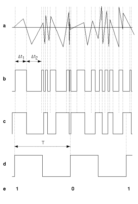
Figure 2: Signals at different points of the hardware generator: a) analog diode noise, b) output of the comparator COMP, c) output Q of the JK flip-flop, d) final output of the generator (D flip-flop).

By setting the control current $I_{c}$ a little lower or higher, the output of the comparator COMP spends respectively a little more or less time in the logical state ”1”. At certain strength of the control current $I_{c}$, one can achieve that the comparator COMP spends approximately equal amount of time in either of the logical states, the point at which the comparator has the highest efficiency of detecting voltage variations. In other words, the duty cycle of the comparator COMP would then on average be close to 0.5. This is ensured by setting $V_{1/2}=\frac{1}{2}V_{DD}$. If, for any reason, the duty cycle ever gets changed, the feedback network closed by comparator COMP, operational amplifier OPA and low-pass filter LP (Fig. 1) will respond by changing the control current $I_{c}$ so that the duty cycle of 0.5 will be restored. This behavior effectively solves the requirement 2. Already here, at the output of the comparator COMP, there is an approximately equal chance that the state is at logical ”0” or at logical ”1”, i.e. the bias of the sampled output would be close to zero. However, due to technical reasons it is quite difficult to keep the bias below 1/1000 for long term and even this would be not possible without some fine-tuning. Tuning the bias consumes a lot of time (due to its statistical nature) and would therefore be unfavorable for a mass production of the generator.

Present method for extracting random bits eliminates the need to tune the bias to zero value, and actually allows to achieve bias as low as desired, without the need to do any modifications to the circuit.

Event counting is the crucial point of the method. Namely, the JK-type flip-flop (Fig. 1) performs a continued counting of the events, but keeps track only whether the count is even or odd. The result of the counting appears at the output Q of the JK flip-flop and represents a new random bit sequence with highly suppressed bias and serial correlation. To understand how this works it is important to keep in mind that the output Q of the JK flip-flop shall be sampled periodically in time. This is a condition for good operation of this generator. The sampling is done by the D-type flip-flop.

Without the loss of generality, let us suppose that at the time zero ($t=0$) the Zener diode Z exhibits a voltage breakdown. (Voltage breakdown is only one of the processes that may cause fluctuations of the voltage across the diode that are manifested as noise. But to simplify the language we will refer to ”voltage breakdown” as a synonym for a sudden positive jump of the voltage across the Zener diode.) This causes the output of the comparator COMP to exhibit a positive going transition (and later a negative one). Every such event triggers the JK flip-flop to reverse its state at the output Q. This is illustrated in the Fig. 2.b and 2.c.

Let us suppose that the voltage breakdowns happen at times $t_{0}$ = 0, $t_{1}$, $t_{2}$, $t_{3}$, $t_{4}$, etc. Tiny intervals of time between neighboring voltage breakdowns $\Delta t_{k}=t_{k}-t_{k-1}$ where $k$ = 1, 2, 3… are distributed according to some statistical distribution. The mean value $\mu$ of duration of this tiny intervals is defined as:

$$\mu=\lim_{N\rightarrow\infty}\frac{1}{N}\sum_{k=1}^{N}t_{k}$$ (8)

For example, in the pure Quantum Mechanical regime of the Zener diode, intervals between neighboring voltage breakdowns $\Delta t_{k}$ follow the Exponential distribution. Mixing of the Quantum Mechanical model with the plasma noise, noise sources other than a Zener diode or other models including effective memory and/or filtering of the noise signal prior to digitization, may lead to more centered distributions such as Poisson or even Uniform-like distribution. The power of this method lies in the fact that the knowledge of the actual distribution of the time intervals between neighboring voltage breakdowns is irrelevant. The only important thing is that the shape of the distribution stays stable over a period of time substantially larger than the sampling period $T$.

The method presented in this work consists in sampling (i.e. reading out) of the output Q of the JK flip-flop periodically, at times $T$, $2T$, $3T\ldots$ and generally at times $i\times T$ with $i=1,2,3\ldots$ . The sampling is made by a D-type flip-flop (Fig. 1). Namely, when a positive-going edge of the sampling signal (that is transition from ”0” to ”1”) appears at the ”Request” input, state that is present at the input D gets sampled. Sampled value is memorized (frozen) and displayed at the output Q of the D-type flip-flop, and stays there until a new positive-going edge appears. According to the definition of the D-type flip-flop, the sampling is done almost instantaneously so its output stays frozen for almost the whole sampling period $T$ which makes possible for other devices (such as a computer) to read it safely.

Let us now suppose that the sampling period $T$ is chosen large enough so that many voltage breakdowns occur during each sampling period. In another words, we suppose:

$$T\gg\mu.$$ (9)

This situation is illustrated in the Fig. 2 where several voltage breakdowns in the noise signal (FIG.2.a) happen during any sampling period of length $T$ (FIG 2.d).

Furthermore, let us denote that the JK flip-flop changes its state at the output Q: $N_{0}$ times from $t=0$ till $t=T$, $N_{1}$ times from $t=T$ till $t=2T$, and generally $N_{i}$ times from $t=iT$, till $t=(i+1)T$, where $i=1,2,3,\ldots$ .

Now we can conclude that every sampling period (of length $T$) approximately equals the sum of many tiny intervals $\Delta t_{k}$:

$$T \approx \sum_{k=1}^{N_{0}}\Delta t_{k}$$

$$T \approx \sum_{k=N_{0}+1}^{N_{0}+N_{1}}\Delta t_{k}$$

$${\rm etc.}$$ (10)

The above equalities hold only approximately because the first and the last of the tiny intervals in a given sum may be only partially happening during the respective sampling period $T$. In such a case, a part of the first tiny interval may have actually happened during the previous period, while a part of the last tiny interval may have actually happened during the next period (sum). However, approximation can be made arbitrarily good by setting the large enough sampling period $T$.

The Central limit theorem of the Statistics states that the sum of a large number (say $N$) of independent random variables (for example $\Delta t_{k}$), which follow some (any) distribution, approaches Normal distribution in the limit of large $N$. This means that the statistical variable $x$ defined as:

$$x=\sum_{k=1}^{N}\Delta t_{k},$$ (11)

follows approximately the Normal distribution for large $N$. However, in our case, defined by equations (10), the ”variable” $x$ is fixed (being just $T$), and the relevant statistical random variable becomes the number of summands, $N$ defined as:

$$\sum_{k=1}^{N}\Delta t_{k}\leq x<\sum_{k=1}^{N+1}\Delta t_{k}.$$ (12)

In the special case mentioned above, when the tiny intervals $\Delta t_{k}$ are distributed according to the Exponential distribution, random variable $N$ follows, by definition, the Poisson distribution:

$$P(N)=\frac{(T/\mu)^{N}}{N!}exp(-T/\mu).$$ (13)

Quite generally, regardless of the distribution function of tiny intervals $\Delta t_{k}$, it can be shown Stip that the integer random variable $N$ is distributed according to the Binomial distribution $B(N;2T/\mu,p)$, where $p$ quickly approaches 0.5 as $T/\mu$ tends to infinity. Given the general expression for the Binomial distribution:

$$B(r;n,p)=\left(\begin{tabular}[]{c}$n$\\ $r$\end{tabular}\right)p^{r}(1-p)^{n-r}.$$ (16)

distribution of the variable $N$ can be written as:

$$B(N;2T/\mu,p)=\left(\begin{tabular}[]{c}$2T/\mu$\\ $N$\end{tabular}\right)p^{N}(1-p)^{2T/\mu-N}.$$ (19)

This is not in a contradiction with the previous result because the Poisson distribution (13) becomes equal to the Binomial distribution (19) in the limit $T/\mu\rightarrow\infty$.

Even without a rigorous proof it is easy to understand why $N$ follows symmetric Binomial distribution (19) in the limit of slow sampling or, equivalently, large $N$. Following eq. (12), for large $N$ we can write:

$$x\approx\sum_{k=1}^{N}\Delta t_{k}.$$ (20)

Approximating the definition (8) with:

$$\mu\approx\frac{1}{N}\sum_{k=1}^{N}\Delta t_{k}$$ (21)

to eliminate the sum in (20) we may conclude:

$$N\approx\frac{1}{\mu}x.$$ (22)

Since $x$ follows Normal p.d.f. so should $N$. But since $N$ is an integer number it actually follows a discrete version of the Normal p.d.f., i.e. symmetric Binomial distribution with $p$=0.5, Q.E.D. This is a very important result because it means that (19) holds regardless of the distribution of tiny intervals $\Delta t_{k}$. This solves the requirement 1.

It can be shown Stip that as a special consequence of the equation (19) the probability that the random variable $N$ is even becomes equal to the probability that it is odd, in the limit $T/\mu\rightarrow\infty$. But, when the JK flip-flop changes its state an even number of times its output Q returns to the initial state (say ”0”) whereas when it changes an odd number of times it returns the complementary state (say ”1”). Thus, in the limit of slow sampling, the probability of producing ”0” would be equal to the probability of producing ”1” at the output Sample (Fig. 1). This fact can be expressed like this:

$$T/\mu\rightarrow\infty\Rightarrow b\rightarrow 0.$$ (23)

Thus it has been shown that the generator and the corresponding method of sampling random phenomena solve the first problem stated in the section 2, i.e. that the bias should vanish in some limit.

The second problem, namely the statistical independence of the logical states (bits) at the output of the generator, is solved as follows. First we realize that the subsequent voltage breakdowns in the Zener diode are statistically independent because the breakdown itself is an unpredictable physical phenomenon. Secondly, the internal capacitive memory that appears in the circuit (which for example may be introduced by imperfections in electronics design, or be a part of physical process governing the alternate current noise source) ”dies off” exponentially with the half-life $\tau$ (Eq. (7)). Effect of the memory on correlations can be made as small as desired in the limit of slow sampling, that is by making T/$\tau$ large enough. Namely, in the limit $T/\tau\rightarrow\infty$ sums of the type (10) become mutually statistically independent. The statistical independence of two subsequent sums, in that limit, takes place because the two sums contain large portion of summands that are ”out of the range” of the memory effect of each other. If we consider two sums that are not subsequent, then the memory effects are even smaller. This means that a bit corresponding to a sum becomes statistically independent of neighboring and even more all other bits, in the limit of slow sampling. It can be concluded that the generator and the corresponding method of sampling random phenomena also solve the second problem stated in the section 2.

Functioning of the whole circuit in Fig. 1 can be best understood by looking at signals shown in the Fig. 2a-e. One can see that with each positive-going edge at the output of the comparator COMP (Fig. 2.b), the JK flip-flop changes state at its output Q (Fig. 2.c). The sampling signal (Fig. 2.d) isn’t, of course, in any synchronization with these signals. Whenever it exhibits a positive-going transition, the output Q of the JK flip-flop gets sampled and the state thus obtained is the output bit from the generator (Fig. 2.e).

It is important to understand that the output Q of the JK flip-flop always produces ”1” after ”0” and ”0” after ”1”, therefore its output is not random at all. However a duration of zeros and ones varies randomly (Fig. 2c) and periodic sampling of the said output by the D-type flip-flop provides a good quality random bits, in the limit of slow sampling ($T\gg\mu$ and $T\gg\tau$).

4 Simulations

In order to check the theory of operation described above, a series of simulations of the circuit in Fig. 1 were made. Simulations should provide an insight on how the type of distribution of tiny intervals between subsequent physical events and ratios $T/\tau$ and $T/\mu$ influence the quality of generated bits. The circuit was simulated by a specifically designed computer program which simulates a random digital signal obeying a specified distribution which would be present at the output of the comparator COMP, and assuming that this signal gets processed by ideal flip-flops. The approximation of considering the two flip-flops to be ideal is very good because their fall and rise times (of approximately 7 nanoseconds) are much shorter than the changes in the noise being processed.

Two distributions of tiny intervals were simulated: Exponential and Uniform. Exponential distribution is natural distribution for many processes. Uniform distribution assumes that the intervals between physical events may be between zero and 1 (in arbitrary time units, for example microseconds) and evenly distributed between the two limits. The two distributions are chosen because they are very different: for example Exponential d. is completely non-symmetric and peaked at one value (zero) whereas Uniform d. is symmetric and has no peak, etc. Most processes should obey distributions that are somewhere between those two extremes.

The effect of memory was simulated as a pile up: any two breakdowns closer (in time) than $\tau$ were considered as being just one breakdown happening at the end of the last breakdown. This in effect may chain up more than two events to be seen as one. This is a very faithful model for a noise source which we use, and a reasonable approximation for any other noise source because memory (by definition) always piles up events in a way that events which happen to close to one another get piled up and be detected as just one event.

The method for extracting bits does not prefer zeros nor ones, therefore we do not expect the bias to be significant even in the case when both ratios $T/\tau$ and $T/\mu$ are small. What happens however is that when sampling is being made too fast there is an excess of longer patterns of ones or zeros. This in turn means that the probability of single ones (pattern ”010”) a well as that of single zeros (pattern ”101”) will be smaller than expected (expected vales are: $p(010)=p(101)=1/8$).

For each choice of distribution, ratio $T/\tau$ and ratio $\tau/\mu$, the program calculates (by simulation) three output values: probability of ones $p(1)$, probability of single ones $p(010)$ and serial correlation coefficient $a$. Results of simulations for the two distributions and a range of ratios $T/\tau$ and $\tau/\mu$ are shown in the tables 3-6. Values shown are bias ($b=p(1)-0.5$), second order bias ($b_{010}=p(010)-0.125$), and serial correlation coefficient. Number of bits generated in each simulation is 6,250,000. According to that statistics, 1 sigma errors are: 0.00020 for $b$, 0.00007 for $b_{010}$ and 0.00040 for $a$. As a source of random numbers the program used semi-hardware ”/dev/urandom” Linux kernel random bit generator. The result were cross-checked using the standard implementation of ”secure” software random number generator rand() that is part of the Linux C compiler (we used gcc version 2.95). No discrepancies were found in the results within the error margins.

	$\tau/\mu$
$T/\mu$	0	0.2	0.33	0.5	0.75	1
2	0.00013	0.00010	-0.00007	0.00030	-0.00029	0.00004
3	-0.00030	0.00028	-0.00010	0.00026	-0.00013	0.00041
4	-0.00005	0.00019	0.00022	-0.00020	-0.00003	-0.00030
6	-0.00000	0.00036	-0.00015	0.00001	0.00020	0.00013
9	0.00011	-0.00005	0.00012	0.00003	-0.00005	-0.00029
12	-0.00013	0.00010	-0.00013	-0.00027	0.00037	-0.00013

Table 1: Uniform distribution, bias

	$\tau/\mu$
$T/\mu$	0	0.2	0.33	0.5	0.75	1
2	0.00955	0.00442	0.00383	0.01479	0.06978	0.10538
3	-0.01351	-0.01744	-0.02429	-0.04041	-0.05231	-0.02093
4	0.00701	0.01220	0.01852	0.02598	-0.00794	-0.03638
6	-0.00100	-0.00121	-0.00227	-0.01113	-0.01609	0.01694
9	0.00028	-0.00001	0.00015	-0.00224	-0.00261	0.00509
12	0.00006	0.00000	0.00015	-0.00038	0.00017	-0.00049

Table 2: Uniform distribution, b(010)

	$\tau/\mu$
$T/\mu$	0	0.2	0.33	0.5	0.75	1
2	-0.05748	-0.04355	-0.05233	-0.11648	-0.31369	-0.40496
3	0.06358	0.08214	0.11607	0.20639	0.27048	0.06288
4	-0.03136	-0.05413	-0.08151	-0.11538	0.01226	0.17930
6	0.00477	0.00503	0.01013	0.05077	0.07227	-0.07653
9	-0.00004	0.00024	-0.00057	0.00963	0.01214	-0.02286
12	0.00044	0.00017	-0.00077	0.00152	-0.00170	0.00254

Table 3: Uniform distribution, serial correlation

	$\tau/\mu$
$T/\mu$	0	0.2	0.33	0.5	0.75	1
2	0.00003	0.00023	-0.00025	0.00013	0.00033	0.00005
3	0.00018	-0.00013	0.00003	-0.00016	0.00034	0.00006
4	-0.00010	-0.00033	-0.00013	-0.00014	-0.00013	0.00005
6	0.00002	-0.00013	-0.00013	0.00022	-0.00013	-0.00016
9	-0.00013	0.00029	0.00014	-0.00011	-0.00016	0.00018
12	-0.00021	-0.00001	0.00002	-0.00000	0.00032	0.00024

Table 4: Exponential distribution, bias

	$\tau/\mu$
$T/\mu$	0	0.2	0.33	0.5	0.75	1
2	-0.00398	-0.00101	0.00168	0.01385	0.04992	0.04163
3	-0.00080	0.00008	-0.00016	-0.00299	0.00777	0.04519
4	0.00016	-0.00015	0.00014	-0.00013	-0.00939	0.00454
6	0.00008	-0.00001	0.00005	-0.00011	0.00209	-0.00742
9	-0.00017	0.00000	-0.00002	-0.00007	-0.00029	0.00139
12	0.00002	-0.00006	-0.00003	-0.00008	-0.00020	-0.00045

Table 5: Exponential distribution, b(010)

	$\tau/\mu$
$T/\mu$	0	0.2	0.33	0.5	0.75	1
2	0.01869	0.00423	-0.00729	-0.06256	-0.20970	-0.20169
3	0.00306	0.00016	0.00042	0.01389	-0.03947	-0.19117
4	-0.00001	0.00033	-0.00016	0.00084	0.04353	-0.02615
6	-0.00058	-0.00029	-0.00023	0.00021	-0.00972	0.03569
9	0.00052	-0.00021	0.00020	0.00022	0.00095	-0.00623
12	0.00033	0.00032	0.00021	0.00006	0.00015	0.00125

Table 6: Exponential distribution, serial correlation

As expected, bias is always consistent with zero. Absolute values of the second order bias and the serial correlation coefficient quickly drop to zero (within the error margins) when the sampling period becomes large enough and memory effects small enough. The Exponential distribution seems slightly more favorable in this respect than the Uniform. From these results it can be concluded that in the worst case good bits are achieved by generators with the memory effect $\tau/\mu<0.33$ and the ratio $T/\mu>9$. This means that using a standard Zener diode with 3 MHz mean frequency of voltage turnovers it should be possible to build a generator that is capable of generating up to several hundred kilobits of good-quality random bits per second.

5 Prototype testing

We have constructed a prototype based on the block-diagram in Fig. 1 using a Zener diode, standard analog chips and CMOS logic. Bits were produced at 300 kbit/sec. We built four identical circuits and fed their outputs to a PC computer, thus obtaining a total of 1.2 Mbit/sec. Thanks to such a high speed we were able to easily produce long sequences of bits for the subsequent testing. The sequences of bits produced by the physical generator were tested by three batteries of statistical tests: Walker’s ENT ENT , Marsaglia’s DIEHARD DIEHARD and NIST’s Statistical Test Suite sts-1.50 .

The ENT consists of battery of standard tests: entropy, Chi-square, mean value, Monte Carlo pi value test and the serial correlation test. These tests may be evaluated for short sequences thus making possible a fast check of the prototype in the development stage. The most important of them are the mean value and the serial correlation test because they best grasp problems in hardware. The mean value addresses the inequality between number of ones and zeros which is very hard to keep close to zero with imperfect hardware. Non zero serial correlation reflects existence of a short-term memory in the system, as explained in the section 3. Indeed, at the development stage of the prototype a slight consistent bias (positive, of the order of $10^{-4}$) has been noticed on all four gadgets which was attributed to the fact that comparator had quite a different rise time from the fall time at its output. This was corrected by taking another comparator after which the bias became undetectable.

Once the generator was debugged and ENT tests passed well, we proceeded by generating long sequences (approx. 10⁸ bits) needed by the DIEHARD, probably the stringiest battery of tests known today. Table 7 shows a typical result of testing of $8\times 10^{7}$ bits (10 megabyte) of random data obtained from the generator.

Test name	p-value
BIRTHDAY SPACINGS	0.6562
OVERLAPPING 5-PERMUTATION	0.4666
OVERLAPPING 5-PERMUTATION	0.5396
BINARY RANK 31x31	0.4256
BINARY RANK 32x32	0.0246
BINARY RANK 6x8	0.1513
BITSTREAM TEST	0.5340
OPSO	0.2728
OQSO	0.6959
DNA	0.8619
COUNT THE 1’s	0.6046
COUNT THE 1’s	0.3398
PARKING LOT	0.7513
MINIMUM DISTANCE	0.2088
3D SPHERES	0.2800
SQUEEZE	0.9366
OVERLAPPING SUMS	0.9472
RUNS UP	0.3664
RUNS DOWN	0.8111
RUNS UP	0.4229
RUNS DOWN	0.5369
CRAPS (wins)	0.2463
CRAPS (throws)	0.1541

Table 7: Typical result of the DIEHARD tests for the hardware non-deterministic generator

According to Marsaglia DIEHARD sequence has failed a test if the p-value of that test is very close to 1 ($p>0.999999$), otherwise the sequence has passed the test. There are 15 different tests in the DIEHARD, but some are run more than once with different parameters (eg. binary rank test) or on independent parts of the sequence under test (eg. count the 1’s). Results in the table 7 indicate a random sequence that has passed all the tests.

It is interesting to note that efforts to standardize requirements for random bit generators for use with cryptographic software have been taken, notably the recommendations of NIST FIPS140-1 . A sequence of 10⁹ bits divided in 100 equally long pieces (files) has been subjected to the NIST’s battery of randomness tests, version sts-1.50 sts-1.50 . We used the recommended test parameters. Results are summarized in the Table 8.

Test#	p-value	Pass rate	Statistical test
1.	0.9240	0.9900	Frequency
2.	0.8165	0.9900	Block-Frequency
3.	0.8343	0.9900	Cusum
4.	0.0456	1.0000	Runs
5.	0.3041	0.9900	Long-Run
6.	0.7197	0.9900	Rank
7.	0.3504	0.9900	FFT
8.	0.0909	1.0000	Aperiodic-Template
9.	0.7791	0.9900	Periodic-Template
10.	0.2022	0.9900	Universal
11.	0.9240	0.9800	Apen
12.	0.8623	1.0000	Random-Excursion
13.	0.7727	0.9844	Random-Excursion-V
14.	0.8831	0.9900	Serial
15.	0.2022	0.9900	Lempel-Ziv
16.	0.8165	0.9900	Linear-Complexity

Table 8: Test of randomness extracted from heartbeats

According to the NIST analysis program, the minimum pass rate for each statistical test with the exception of the random excursion (variant) test is approximately 0.9602 whereas the minimum pass rate for the random excursion (variant) test is approximately 0.9527. Taking this into account we conclude that all 16 tests were passed with excellent marks. Passing all three batteries of tests shows that this generator conforms also to the general requirement 4 stated in the section 3.

As one more check of the sampling method itself bits were generated from a cardiogram data of a healthy patient. A record of 1190 consequent heartbeats was made in course of an ergometric stress test. During the test patient is required to walk on a treadmill whose speed varies according to a standardized procedure. Test lasts approximately 12 minutes. The times at which main heartbeat peaks occur were considered as physical ”events”. Taking $T/\mu\approx 5$ we obtained a sequence of 216 bits using our method. Results of ENT test shown in the table 9 indicate excellent randomness. This demonstrates the power of the method which is able to extract good random bits form a sequence of heartbeats which are nearly periodic but have only a slight random jitter.

Bit entropy	Chisquare	Mean value	Serial correlation
0.9977	$0.67/50$%	$0.528\pm 0.034$	$-0.003\pm 0.069$

Table 9: Test of randomness extracted from heart beats

The conclusion is that heartbeat timings may very well be used as a base for a non-deterministic random generator !

6 Conclusion

A method for extraction of non-deterministic random bits from random physics processes (such as nuclei decay or noise voltage variations) is presented. The method is characterized by the fact that it ensures a good quality random bits in an easily obtainable limit, that is the limit of slow sampling, regardless of the distribution of times between adjacent processes. A physical random bit generator which makes use of the method and Zener diode noise was built and successfully tested. The generator is shown to conform to general requirements for non-deterministic generators stated in section 3. A sample of approximately $10^{9}$ bits produced by the physical generator prototype is subjected to a series of well-known statistical tests showing no weaknesses.

7 Acknowledgments

The heartbeat recording was provided by courtesy of M. Martinis from Rudjer Bošković Institute and the Institute for cardiac deseases, Zagreb. These data were taken with approval of the patient.

Parts of the method and apparatus for producing random bits are subjected to a patent procedure.

References

- (1) M.A. Nielsen, I.L. Chuang, Quantum Computation and Quantum Information, (Cambridge University Press, Cambridge, 2000) p. 2.
- (2) Wikipedia, the free encyclopedia, Internet URL: http://www.wikipedia.org/wiki/Probabilistic_Turing_Machine
- (3) M. J. Atallah, Algorithms and Theory of Computation Handbook, (CRC Press LLC, Boca Raton, 1998) p. 29.
- (4) W. H. Press, B. P. Flannery, S. A. Teukolsky, W. T. Vetterling, Numerical Recipes in C: The Art of Scientific Computing, (Cambridge University Press, New York, 1992)
- (5) D. E. Knuth, The art of computer programming, Vol. 2, Third edition, (Addison-Wesley, Reading, 1997)
- (6) M. Luescher, Comp. Phys. Comm, 79(1994) 100.
- (7) F. James, Comp. Phys. Comm. 79(1994) 111.
- (8) P. Hellekalek, Mathematics & Computers in Simulation 46(1998) 485.
- (9) W. E. Sharp, C. Bays, Computers & Geosciences, 18(1992) 79.
- (10) A.J. Miller, P. Mars, Mathematics & Computers in Simulation, 19(1997) 198.
- (11) G. Marsaglia, Statistics & Probability Letters, 9(1990) 345.
- (12) S. Agostinelli et. al, Nucl. Instr. and Meth. A 506(2003) 250.
- (13) M. O. Rabin, J. Number Th. 12(1980) 128.
- (14) C. H. Bennet, G. Brassard, Quantum cryptography: Public key distribution and coin tossing, Proceedings of IEEE International Conference on Computers, Systems and Signal Processing, (IEEE, New York, 1984) p. 175.
- (15) U. Maurer, IEEE Transactions on Information Theory, 39 (1993) 733.
- (16) R. L. Rivest, The RC4 Encryption Algorithm, RSA Data Security Inc., Mar. 12, 1992.
- (17) I. Goldberg, D. Wagner, Dr. Dobb’s, January 1996
- (18) D. Davis, R. Ihaka, P. Fenstermacher, Cryptographic Randomness from Air Turbulence in Disk Drives in: Lecture Notes in Computer Science Springer Verlag, Berlin, 1984) p. 839.
- (19) D. Eastlake, S. Crocker, J. Schiller, Randomness Recommendations for Security, Internet RFC 1750, December 1994.
- (20) T. Ts’o, private communication. See also Linux man page urandom(4) and source code of Linux kernel ver. 2.4.18, file random.c
- (21) C. H. Vincent, J. Phys. E 3(1970) 594.
- (22) V. Bagini, M. Bucci, A design of Reliable True Random Number Generator for Cryptographic Applications, in: Proceedings of CHES’99 Workshop, (Springer Verlag, Berlin ,2000) p. 204.
- (23) Security Requirements for Cryptographic Modules, Federal Information Processing Standards Publication 140-1, (FIPS, Gaithersburg, 1994)
- (24) P. I. Somlo, Electronics Letters, 11 (1975) 290.
-
(25)
M. Stipčević,
Some properties of inverted distributions and their application in sampling random phenomena,
to appear in the Cryptology ePrint Archive, Internet URL:
http://eprint.iacr.org -
(26)
ENT - A Pseudorandom Number Sequence Test Program, J. Walker, Internet URL:
http://www.fourmilab.ch/random/ -
(27)
DIEHARD battery of stringent randomness tests (various articles and software), G. Marsaglia, Internet URL:
http://stat.fsu.edu/~geo/diehard.html, also available on CDROM online - (28) A. Rukhin et. al., A Statistical Test Suite for Random and Pseudorandom Number Generators for Cryptographic Applications, NIST Special Publication, (NIST, Gaithersburg, 2001)