Mode Competition in Gas and Semiconductor Lasers

Abstract

The output spectrum of both gas and semiconductor lasers usually contains more than one frequency. Multimode operation in gas versus semiconductor lasers arises from different physics. In gas lasers, slow equilibration of the electron populations at different energies makes each frequency an independent single-mode laser. The slow electron diffusion in semiconductor lasers, combined with the spatially varying optical intensity patterns of the modes, makes each region of space an independent single-mode laser. We develop a rate equation model for the photon number in each mode which captures all these effects. Plotting the photon number versus pumping rate for the competing modes, in both subthreshold and above threshold operation, illustrates the changes in the laser output spectrum due to either slow equilibration or slow diffusion of electrons.

1 Introduction

The basic physics of mode competition in gas and semiconductor lasers has been known since the 1960’s [1]- [4]. When the laser medium is in quasi-equilibrium and spatial variations in the mode patterns can be neglected, only a single frequency appears in the laser output. A rate equation model developed by Siegman [2, 3] describes the subthreshold, transition, and lasing regions of operation for a single mode laser. Quantum theories of a single mode laser [5] give similar (if not idential) results for the laser output power versus pumping rate as the simpler semiclassical models.

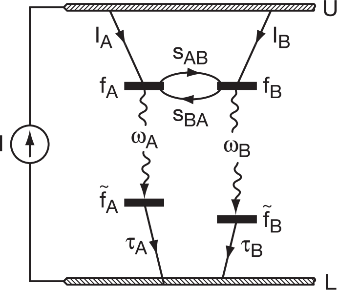
Figure 1: A four level lasing system representing both gas and semiconductor lasers. A current $I$ pumps electrons from a lower thermodynamic reservoir ($L$) into an upper electron bath ($U$). Currents $I_{A}$ ($I_{B}$) then transfer electrons into the upper level of transition $A$ ($B$). An electron electron scattering rate $s_{AB}$ ($s_{BA}$) from the upper levels of transition $A$ to transition $B$ ($B$ to $A$) is also present in this model. The upper lasing levels has occupation factor $f_{A}$ ($f_{B}$), while the occupation factor of the lower lasing level is assumed to be $\tilde{f}_{A}=0$ ($\tilde{f}_{B}=0$).

In this paper we extend the rate equation models for a single model laser [2, 3] to include mode competition in both gas and semiconductor lasers. For the gas laser we develop a set of coupled rate equations which allow electron scattering between the lasing levels. The slow electron scattering rate in gas lasers allows the electron occupation factors in the different lasing levels to get out of equilibrium with each other, producing multiple frequencies in the laser output. In semiconductor lasers electron scattering between the different energy levels is rapid, keeping the occupation factors in the different lasing levels in equilibrium with each other. But spatial variation in the optical mode intensities inside the laser cavity favor different lasing modes in different regions of space within the semiconductor. Following Ref. [4] we extend the rate equations for a homogenous (semiconductor) line to allow for spatially varying mode patterns, generating multiple frequencies in the laser output.

We assume both gas and semiconductor lasers are a four level system, with two intermediate lasing levels, as shown in Fig. 1. For simplicity we consider only two lasing modes, mode $A$ and mode $B$, with mode $A$ the favored lasing mode. For the gas laser $A$ and $B$ represent localized atomic states, while for the semiconductor $A$ and $B$ are spatially extended states within the energy band of a quantum well. To simplify the mathematics we assume lower lasing level is always empty, having occupation factors $\tilde{f_{A}}=\tilde{f_{B}}=0$. In the language of gas lasers this means we assume electrons in the lower lasing level empty very efficiently into an electron bath ($\tau_{A}\;,\tau_{B}\to 0$). In semiconductor language we would say there is extremely efficient hole capture into the quantum well. We therefore consider only pumping electrons into the upper lasing level. In physical systems would also have to guarentee charge neutrality while pumping the laser, and therefore also consider details of pumping and relaxation out of the lower lasing level.

In this paper we limit consideration of laser mode competition to only 1-2 competing modes. In actual lasers many modes compete, and this case has been considered by Casperson [6]. The rate equation models in this paper can be easily generalized to consider multiple lasing modes.

2 Gas Lasers: Spectral Hole Burning

We construct the rate equations for an inhomogeneous line following the example of a single mode laser from Refs. [2, 3]. We consider a scattering rate $s_{A\to B}=s_{AB}$ for electrons from mode $A$ to mode $B$. If we firstly neglect optical transitions, the rate equation for the occupation probability $f_{A}$ for electrons in state $A$ is

$$\frac{df_{A}}{dt}=-f_{A}s_{AB}(1-f_{B})+f_{B}s_{BA}(1-f_{A})+I_{A}.$$ (1)

Here $I_{A}$ is the pumping current per state. Specializing to thermodynamic equilibrium (no pumping current) implies the rates $s_{AB}$ and $s_{BA}$ are related by a Boltzmann factor as

$$s_{AB}=s_{BA}\exp{(E_{A}-E_{B})/k_{B}T}.$$ (2)

The rate equation for the photon number $n_{A}$ in mode A is unchanged from that for a single mode laser

$$\frac{dn_{A}}{dt}=K_{A}(n_{A}+1)N_{A}-\gamma_{A}n_{A}.$$ (3)

Here $K_{A}$ is an optical rate constant for the $A$ transition, $N_{A}$ the number of $A$ states (number of atoms of type $A$ in a gas laser), and $\gamma_{A}$ the cavity escape rate for photons having frequency $\omega_{A}$. Putting Eqs. (1)-(3) together (along with analogous equations for mode $B$) into a single matrix equation for the variables $f_{A}$, $f_{B}$, $n_{A}$, and $n_{B}$ gives

$$\frac{d}{dt}\left[\begin{array}[]{c}f_{A}\cr\\ f_{B}\cr\\ n_{A}\cr\\ n_{B}\cr\end{array}\right]=\left[\begin{array}[]{cccc}\begin{array}[]{c}-(K_{A}n_{A}+A_{A}+s_{AB})\\ +(s_{AB}-s_{BA})f_{B}\end{array}&s_{BA}&0&0\\ s_{AB}&\begin{array}[]{c}-(K_{B}n_{B}+A_{B}+s_{BA})\\ +(s_{BA}-s_{AB})f_{A}\end{array}&0&0\\ \\ K_{A}(n_{A}+1)N_{A}&0&-\gamma_{A}&0\cr\\ 0&K_{B}(n_{B}+1)N_{B}&0&-\gamma_{B}\cr\\ \end{array}\right]\left[\begin{array}[]{c}f_{A}\cr\\ f_{B}\cr\\ n_{A}\cr\\ n_{B}\cr\end{array}\right]+\left[\begin{array}[]{c}I_{A}\cr\\ I_{B}\cr\\ 0\cr\\ 0\cr\end{array}\right].$$ (4)

We now specialize to $(E_{A}-E_{B})\ll k_{B}T$ so that we can approximate $s_{AB}\simeq s_{BA}=s$. As scattering rate $s$ becomes large ($s\to\infty$), the occupation factors $f_{A}$ and $f_{B}$ are forced to equal each other $(f_{A}=f_{B})$ in this approximation. Without the approximation $s_{AB}\simeq s_{BA}$, and in the absence of any optical transitions, we would have the occupation factors forced towards a Fermi distribution $f(E)$ having $f_{A}=f(E_{A})$ and $f_{B}=f(E_{B})$ as $s_{AB}\to\infty$. The approximation $s_{AB}\simeq s_{BA}$ therefore makes only a minor correction to the occupation factors, and is therefore not essential for our analysis of mode competition. We therefore approximate $s_{AB}\simeq s_{BA}=s$ leading to

$$\frac{d}{dt}\left[\begin{array}[]{c}f_{A}\\ f_{B}\\ n_{A}\\ n_{B}\end{array}\right]=\left[\begin{array}[]{cccc}-(K_{A}n_{A}+A_{A}+s)&s&0&0\\ s&-(K_{B}n_{B}+A_{B}+s)&0&0\\ K_{A}(n_{A}+1)N_{A}&0&-\gamma_{A}&0\\ 0&K_{B}(n_{B}+1)N_{B}&0&-\gamma_{B}\end{array}\right]\left[\begin{array}[]{c}f_{A}\\ f_{B}\\ n_{A}\\ n_{B}\end{array}\right]+\left[\begin{array}[]{c}I_{A}\\ I_{B}\\ 0\\ 0\end{array}\right].$$ (5)

Inspection of the upper left quadrant of the matrix in Eq. (5) shows that the scattering rate $s$ is negligible until $s$ exceeds one of the spontaneous emission rates $A_{A}$ or $A_{B}$. Thus, the transition from two independent lasers ($s=0$) to a homogeneous line ($s\to\infty$) occurs when the scattering rate $s$ exceeds the spontaneous emission rates $A_{A}$ and $A_{B}$. This is true in open cavity lasers with luminescence through the sides of the laser cavity, so that the spontaneous emission rates $A_{A}$ and $A_{B}$ greatly exceed the cavity escape rates $\gamma_{A}$ and $\gamma_{B}$. If the cavity is closed, so that no side luminescence occurs, the spontaneous emission rates are forced towards the cavity rates, i.e. $A_{A}\to\gamma_{A}$ and $A_{B}\to\gamma_{B}$. In the case of a closed cavity the transition from two independent lasers to a homogeneous line occurs when the scattering rate $s$ is comparable to the cavity rates $\gamma_{A}$ and $\gamma_{B}$. Note that on a homogeneous line $(s\to\infty)$ Eq. (5) simplifies to $f\equiv f_{A}=f_{B}$ and

$$\frac{d}{dt}\left[\begin{array}[]{c}2f\\ n_{A}\\ n_{B}\end{array}\right]=\left[\begin{array}[]{cccc}-(K_{A}n_{A}+K_{B}n_{B}+A)&0&0\\ K_{A}(n_{A}+1)N_{A}&-\gamma_{A}&0\\ K_{B}(n_{B}+1)N_{B}&0&-\gamma_{B}\end{array}\right]\left[\begin{array}[]{c}f\\ n_{A}\\ n_{B}\end{array}\right]+\left[\begin{array}[]{c}I\\ 0\\ 0\end{array}\right],$$ (6)

where $I=I_{A}+I_{B}$ and $A=A_{A}+A_{B}$.

We solve Eq. (5) in steady state using an iterative technique. From the $i$th iteration for the variables $f_{A}^{i}$, $f_{B}^{i}$, $n_{A}^{i}$, and $n_{B}^{i}$, we produce the $(i+1)$st iteration by

$$-\left[\begin{array}[]{c}f_{A}^{i+1}\\ f_{B}^{i+1}\\ n_{A}^{i+1}\\ n_{B}^{i+1}\end{array}\right]=\left[\begin{array}[]{cccc}-(K_{A}n_{A}^{i}+A_{A}+s)&s&0&0\\ s&-(K_{B}n_{B}^{i}+A_{B}+s)&0&0\\ K_{A}(n_{A}^{i}+1)N_{A}&0&-\gamma_{A}&0\\ 0&K_{B}(n_{B}^{i}+1)N_{B}&0&-\gamma_{B}\end{array}\right]^{-1}\left[\begin{array}[]{c}I_{A}\\ I_{B}\\ 0\\ 0\end{array}\right].$$ (7)

We have tried several different types of initial guesses for $f_{A}$, $f_{B}$, $n_{A}$, and $n_{B}$ to start the iterative procedure, and the final results seem to be independent of the different initial guesses. The initial guess which seems to converge in the shortest time is to start in the subthreshold region and take for $f_{A}^{i}$, $f_{B}^{i}$, $n_{A}^{i}$, and $n_{B}^{i}$ the analytical results for two independent single mode lasers ($s=0$). When incrementing to the next pumping rate, assume an initial guess for $f_{A}$, $f_{B}$, $n_{A}$, and $n_{B}$ which are just the converged values at the previous pumping rate.

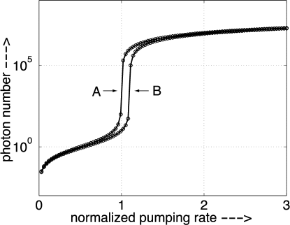
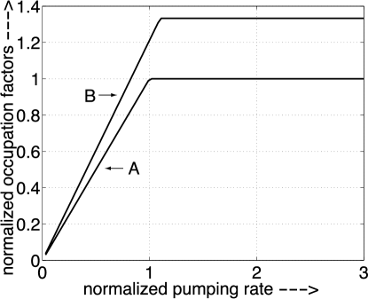
Figure 2: (a) Photon numbers $n_{A}$ and $n_{B}$ and (b) normalized occupation factors $f_{A}/f_{th}^{A}$ and $f_{B}/f_{th}^{A}$ when the electron scattering rate between states $A$ and $B$ is $s=0$. The iterative solution of Eq. (5) (solid lines) matches the analytical solutions for two independent single mode lasers (circles) having $s=0$ from Eqs. (8)-(9).

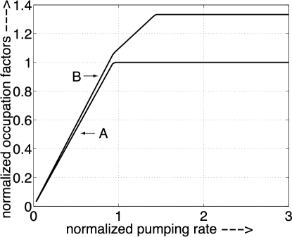
Figure 3: (a) Photon numbers $n_{A}$ and $n_{B}$ and (b) normalized occupation factors $f_{A}/f_{th}^{A}$ and $f_{B}/f_{th}^{A}$ when the electron scattering rate $s$ between states $A$ and $B$ equals the spontaneous emission rate of mode $A$ ($s=1.0A_{A}$). Scattering forces the occupation factors $f_{A}$ and $f_{B}$ towards each other, reducing the threshold current for mode $A$ and increasing the threshold current of mode $B$.

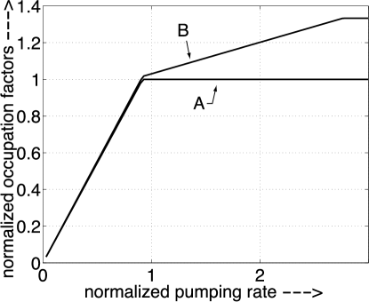
Figure 4: (a) Photon numbers $n_{A}$ and $n_{B}$ and (b) normalized occupation factors $f_{A}/f_{th}^{A}$ and $f_{B}/f_{th}^{A}$ when the electron scattering rate $s$ between states $A$ and $B$ is five times the spontaneous emission rate of mode $A$ ($s=5.0A_{A}$). The threshold current of mode $A$ decreases slightly from Fig. 3, while the threshold current for mode $B$ substantially increases.

We use some results from the single mode laser [2, 3] to frame our discussion of two coupled lasing modes. When the two laser modes are decoupled ($s=0$), the threshold currents for each mode are $I_{th}^{A}=\gamma_{A}A_{A}/N_{A}K_{A}$ and $I_{th}^{B}=\gamma_{B}A_{B}/N_{B}K_{B}$. The normalized pumping rate $r$ is defined as $r=I_{A}/I_{th}^{A}$. We define the ratio of the two threshold currents when the modes are decoupled as $z=I_{th}^{B}/I_{th}^{A}$. We assume the pumping current divides equally among the two states so that $I_{A}=I_{B}=I/2$. The occupation factors above threshold are fixed at $f_{A}=f_{th}^{A}=\gamma_{A}/N_{A}K_{A}$ and $f_{B}=f_{th}^{B}=\gamma_{B}/N_{B}K_{B}$ due to gain saturation.

An important laser parameter is the number of luminescent modes $p$, where $A_{A}\equiv pK_{A}$. For mode $B$ this leaves the relation $A_{B}\equiv pzK_{B}(\gamma_{A}/\gamma_{B})(N_{B}/N_{A})$. We further simplify by taking $N=N_{A}=N_{B}$ and $\gamma_{A}=\gamma_{B}=\gamma$. In the absence of mode coupling ($s=0$), the results for photon numbers versus normalized pumping rate $r$ are then

$$2n_{A}=p(r-1)+p\sqrt{(r-1)^{2}+(4r/p)}$$ (8)

and

$$2n_{B}=p(r-z)+p\sqrt{(r-z)^{2}+(4r/p)}.$$ (9)

Figures 2-4 show the photon numbers and occupation factors versus normalized pumping rate $r$ for different scattering rates $s$. We choose $p=10^{7}$ and $z=1.1$ in Figs. 2-4. In Fig. 2 there is no scattering between states $A$ and $B$ ($s=0$), leaving two independent single mode lasers. Iterating Eq. (7) (solid lines) then just reproduce the analytical results from Eqs. (8)-(9) (circles) in Fig. 2(a). The normalized occupation factors $f_{A}/f_{th}^{A}$ and $f_{B}/f_{th}^{A}$ in Fig. 2 increase approximately linearly with pumping below threshold and saturate above the lasing threshold.

As the scattering rate increases to $s=1.0A_{A}$ in Fig. 3, and even further to $s=5.0A_{A}$ in Fig. 4, we see the lasing threshold for mode $A$ shifts to a lower pumping current. The threshold current for mode $B$ continues to increase as the scattering rate $s$ increases. The increase in lasing threshold for mode $B$ is much more pronounced than the decrease in threshold current for mode $A$. Inspection of the occupation factors for the two decoupled lasers in Fig. 2(b) explains the threshold current shifts. Increasing the scattering rate $s$ forces the two occupation factors towards each other. In Fig. 2(b) we have $f_{B}>f_{A}$ in the subthreshold region. Hence scattering between the modes will increase $f_{A}$ and decrease $f_{B}$ in the subthreshold region as seen in Fig. 3(b) and Fig. 4(b). Scattering then lowers the threshold current required for mode $A$ to lase. Once mode $A$ reaches the lasing threshold, additional scattering between states $A$ and $B$ makes it more difficult for mode $B$ to raise its occupation factor to $f_{B}=f_{th}^{B}$ required for mode $B$ to lase.

The threshold current for mode $A$ can shift in either direction, up or down, with additional scattering between the modes. If $f_{B}>f_{A}$ in the subthreshold region, the case we have chosen in Figs 2-4, additional scattering $s$ lowers the threshold current for mode $A$. If the occupation factors obey $f_{B}<f_{A}$ in the subthreshold region, then the threshold current for mode $A$ increases with additional scattering $s$. When the pumping current divides equally between the states $A$ and $B$ as we have assumed, the threshold current for mode $A$ shifts down with additional scattering $s$ if $(f_{th}^{B}/I_{th}^{B})>(f_{th}^{A}/I_{th}^{A})$, or, equivalently, if the spontaneous rates obey $A_{A}>A_{B}$. Given our assumptions of $\gamma_{A}=\gamma_{B}=\gamma$ and $N_{A}=N_{B}=N$, we require $K_{A}>zK_{B}$ for additional scattering $s$ to lower the threshold current of mode $A$. Since we choose $z=1.1$ and $K_{B}=0.75K_{A}$ in Figs. 2-4 this condition is satisfied. Increasing $z$ and/or $K_{B}$ could reverse the inequality and raise the threshold current for mode $A$ with increased scattering $s$. If the pumping current divides unequally as $I_{A}=\alpha I$ and $I_{B}=(1-\alpha)I$, the requirement for additional scattering $s$ to lower the threshold current of mode $A$ is $(1-\alpha)A_{A}>\alpha A_{B}$. The threshold current required for mode $B$ to lase will always increase when we add additional scattering $s$ (assuming mode $A$ is the favored lasing mode with $f_{th}^{A}<f_{th}^{B}$).

In the limit of $s\to\infty$ we move towards a homogeneous line. Figure 5 shows the solution of Eq. (5) with with $s=100A_{A}$. The photon number $n_{B}$ and occupation factor $f_{B}$ are now essentially fixed when mode $A$ starts lasing due to gain saturation. Iteratively solving Eq. (6) produces essentially the same graph as shown in Fig. 5. The homogeneous line shown in Fig. 5 is the opposite limit of two independent laser lines shown in Fig. 2. Varying the scattering rate $s$ interpolates smoothly between the solutions in Fig. 2 and Fig. 5.

Figure 5: (a) Photon numbers $n_{A}$ and $n_{B}$ and (b) normalized occupation factors $f_{A}/f_{th}^{A}$ and $f_{B}/f_{th}^{A}$ when the electron scattering rate $s$ between states $A$ and $B$ approaches infinity ($s=100A_{A}$). Since $s\to\infty$ we approach the limit of a homogeneous laser line and of a single mode laser.

3 Semiconductor Lasers: Spatial Hole Burning

When there are spatial variations in the optical intensity in different modes, two lasing frequencies can coexist on a homogeneous line. Figure 6 shows the normalized optical mode intensities $|u_{A}|^{2}$ and $|u_{B}|^{2}$ for the lowest two longitudinal modes in a cavity. Near the center of the laser (region I), mode $A$ is the favored lasing mode. However in region II, where the optical intensity $|u_{B}|^{2}>|u_{A}|^{2}$, mode $B$ is the favored lasing mode. If the gain medium were confined to region I, only mode $A$ would lase. Similarly, for the gain medium restricted to region II, only mode $B$ would lase. For semiconductor lasers the gain media fills the entire laser cavity, so there is competition for the available optical gain between the lasing modes.

Whether or not a single or multiple frequencies appear in the laser output spectrum depends on the size of the electron diffusion coefficient $D$. For single frequency laser operation to occur the electron must diffuse from region I to region II in Fig. 6 before the photon exits the cavity. If the photon escapes the laser cavity before the electron can diffuse from region I to region II, the regions are essentially independent as far as the laser light is concerned. Optically, the laser behaves as if two independent (single mode) lasers operate inside the cavity. The distance from region I to region II in Fig. 6 is approximately one quarter of the lasing wavelength ($\lambda/4$). So for open cavity lasers we expect essentially single mode operation whenever $D\gg(\lambda/4)^{2}\tilde{A}$. If the cavity is closed (no side luminescence) so that $\tilde{A}\to\gamma_{A}$, the condition for single mode laser operation becomes $D\gg(\lambda/4)^{2}\gamma_{A}$.

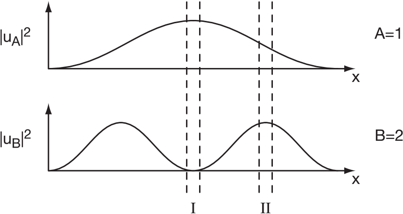
Figure 6: Competition between two lasing modes $A$ and $B$ is possible on a homogeneous line when the optical mode intensities $|u_{A}|^{2}$ and $|u_{B}|^{2}$ vary in space. Mode $A$ is favored in region I, while in region II mode $B$ is the favored lasing mode.

To describe semiconductor lasers quantitatively we need to generalize Eq. (4) to account for the spatial variation in the mode patterns and electron density inside the laser. The occupation factors in each mode will be spatially varying such that $f_{A}\to f_{A}(r)$ and $f_{B}\to f_{B}(r)$. If we introduce the position dependent density of states $N(E,r)$, the total electron density is now

$$\rho(r,t)=\sum_{i}N(E_{i},r)f_{i}(r,t).$$ (10)

The electron density in states $A$ and $B$ are $\rho_{A}(r)=N(E_{A},r)f_{A}(r)$ and $\rho_{B}(r)=N(E_{B},r)f_{B}(r)$. The total number of active type $A$ lasing levels is then

$$N_{A}=\int_{a}N(E_{A},r)dV,$$ (11)

where $\int_{a}$ denotes integration over that portion of the laser cavity containing the active lasing media. We further define the scattering rate per initial and final state density $\tilde{s}_{AB}$ as

$$\tilde{s}_{AB}=\frac{s_{AB}}{N(E_{A},r)N(E_{B},r)}.$$ (12)

To account for spatial variations in the electromagnetic modes inside the laser cavity we introduce the mode functions $u_{A}(r)$ and $u_{B}(r)$ such that the electromagnetic energy density is given

$$\hbar\omega_{A}n_{A}(t)|u_{A}(r)|^{2}=\epsilon(r)|E_{A}(r,t)|^{2},$$ (13)

where $E_{A}(r,t)$ is the electric field of mode $A$ and $\epsilon(r)$ the dielectric constant. Since we must have

$$\int_{L}\epsilon(r)|E_{A}(r,t)|^{2}dV=\hbar\omega_{A}n_{A}(t),$$ (14)

where the integration region $L$ denotes the entire laser cavity, the mode functions $u_{A}(r)$ are normalized as

$$\int_{L}|u_{A}(r)|^{2}dV=1.$$ (15)

We can insert this factor of ’1’ from Eq. (15) wherever necessary in order to generalize Eq. (4) to account for spatially varying electromagnetic fields.

Using Eqs. (10)-(15), the generalization of Eq. (1) to account for spatial variations in the electron density and electromagnetic field intensity is

$$\frac{d\rho_{A}}{dt}=N(E_{A},r)\left\{-\rho_{A}\tilde{s}_{AB}[N(E_{B},r)-\rho_{B}]+\rho_{B}\tilde{s}_{BA}[N(E_{A},r)-\rho_{A}]\right\}$$

$$+R_{A}(r,t)-[K_{A}V_{L}]n_{A}|u_{A}|^{2}\rho_{A}-A_{A}\rho_{A}+D_{A}\nabla^{2}\rho_{A}.$$ (16)

Here $R_{A}(r,t)=N(E_{A},r)I_{A}(r,t)$ is the total pumping rate per unit volume into the state $A$, $V_{L}=\int_{L}dV$ the volume of the laser cavity, and $D_{A}$ the diffusion constant of electrons in state $A$. The generalization of Eq. (3) to account for spatial variations inside the laser is

$$\frac{dn_{A}}{dt}=[K_{A}V_{L}](n_{A}+1)\int_{a}|u_{A}|^{2}\rho_{A}dV-\gamma_{A}n_{A}.$$ (17)

Eqs. (16)-(17) can be used to construct a generalization of the coupled mode Eq. (4) to account for spatial variations in the laser.

Our interest is in semiconductors with homogeneous optical lines, so we do not pursue the full generalization of Eq. (4). We assume the scattering rate $s_{AB}\to\infty$ in the semiconductor, so that we are back on a homogeneous optical line. We assume negligible separation of the energy levels as before so that $(E_{A}-E_{B})\ll k_{B}T$ and $s=s_{AB}=s_{BA}$ The occupation factors we therefore take to be in equilibrium with each other at each point in space so that $f(r)=f_{A}(r)=f_{B}(r)$. With these assumptions we have

$$\frac{d\rho(r,t)}{dt}=-\left([K_{A}V_{L}]n_{A}(t)|u_{A}(r)|^{2}+A_{A}\right)\frac{N(E_{A},r)}{N(E_{A},r)+N(E_{B},r)}\rho(r,t)$$

$$-\left([K_{B}V_{L}]n_{B}(t)|u_{B}(r)|^{2}+A_{B}\right)\frac{N(E_{B},r)}{N(E_{A},r)+N(E_{B},r)}\rho(r,t)$$

$$+D\nabla^{2}\rho(r,t)+R(r,t).$$ (18)

Here $\rho=\rho_{A}+\rho_{B}$ is the total electron density, the total pumping rate is $R=R_{A}+R_{B}$, and we have taken $D=D_{A}=D_{B}$ for the diffusion constant. The final coupled mode rate equations for a homogeneous semiconductor line that we solve are

$$\frac{d\rho}{dt}=-[\tilde{K}_{A}V_{L}]n_{A}|u_{A}|^{2}\rho-[\tilde{K}_{B}V_{L}]n_{B}|u_{B}|^{2}\rho-\tilde{A}\rho+D\nabla^{2}\rho+R,$$ (19)

together with

$$\frac{dn_{A}}{dt}=(n_{A}+1)\int_{a}[\tilde{K}_{A}V_{L}]|u_{A}|^{2}\rho dV-\gamma_{A}n_{A},$$ (20)

and

$$\frac{dn_{B}}{dt}=(n_{B}+1)\int_{a}[\tilde{K}_{B}V_{L}]|u_{B}|^{2}\rho dV-\gamma_{B}n_{B}.$$ (21)

The position dependent optical rate constants $\tilde{K}_{A}(r)$, $\tilde{K}_{B}(r)$, and $\tilde{A}(r)$ are

$$\tilde{K}_{A}(r)=K_{A}\frac{N(E_{A},r)}{N(E_{A},r)+N(E_{B},r)},$$ (22)

with

$$\tilde{K}_{B}(r)=K_{B}\frac{N(E_{B},r)}{N(E_{A},r)+N(E_{B},r)},$$ (23)

and

$$\tilde{A}(r)=\frac{A_{A}N(E_{A},r)+A_{B}N(E_{B},r)}{N(E_{A},r)+N(E_{B},r)}.$$ (24)

Eqs. (19)-(21) are similar to Eqs. (E.1.9a) and (E.1.9b) for a single mode laser from Ref. [4]. Eqs. (19)-(21) should also be considered the generalization of Eq. (6) to account for spatial variations while lasing on a homogeneous line. We simplify further by taking the electron density of states to be constant in space so that the rate constants $\tilde{K}_{A}(r)$, $\tilde{K}_{B}(r)$, and $\tilde{A}(r)$ are independent of space. For simplicity and concreteness we consider competition between the longitudinal laser modes, though the same procedure would work for the inclusion of transverse cavity modes. We choose an Fabry-Perot type cavity having the normalized mode functions

$$|u_{A}|^{2}=\frac{2}{A_{L}L}\sin^{2}(A\pi x/L)$$ (25)

and

$$|u_{B}|^{2}=\frac{2}{A_{L}L}\sin^{2}(B\pi x/L).$$ (26)

Here $A_{L}$ is the cavity area, $L$ the cavity length, $A$ is the number of half wavelengths in mode $A$, and $B$ the number of half wavelengths in the longitudinal cavity mode $B$.

3.1 Slow Diffusion

We solve Eqs. (19)-(21) in steady state using an iterative technique. We take the diffusion constant $D=0$, letting us solve Eq. (19) for $\rho$ and substitute back into Eqs. (20)-(21) leading to

$$n_{A}=(n_{A}+1)p\int_{a}\frac{|u_{A}|^{2}r(dV/V_{a})}{|u_{A}|^{2}n_{A}+|u_{B}|^{2}n_{B}(1/z)+(p/V_{L})},$$ (27)

and

$$n_{B}=(n_{B}+1)p\int_{a}\frac{(1/z)|u_{B}|^{2}r(dV/V_{a})}{|u_{A}|^{2}n_{A}+|u_{B}|^{2}n_{B}(1/z)+(p/V_{L})}.$$ (28)

In Eqs. (27)-(28) we have used the ration of optical coupling constants $z=\tilde{K}_{A}/\tilde{K}_{B}$, the number of luminescent modes $p=\tilde{A}/\tilde{K}_{A}$, assumed equal cavity escape rates $\gamma_{A}=\gamma_{B}$, and defined the normalized pumping rate as $r=R/R_{th}^{A}=RV_{a}/\gamma p$. We now produce the $(m+1)$st iteration for the photon numbers from the $m$th iteration using

$$n_{A}(m+1)=p\int_{L_{a}}\frac{(n_{A}(m)+1)r(x)\sin^{2}(A\pi x/L)(dx/L_{a})}{n_{A}(m)\sin^{2}(A\pi x/L)+(1/z)n_{B}(m)\sin^{2}(B\pi x/L)+(p/2)},$$ (29)

and

$$n_{B}(m+1)=p\int_{L_{a}}\frac{(n_{B}(m)+1)r(x)(1/z)\sin^{2}(B\pi x/L)(dx/L_{a})}{n_{A}(m)\sin^{2}(A\pi x/L)+(1/z)n_{B}(m)\sin^{2}(B\pi x/L)+(p/2)}.$$ (30)

Here $V_{a}=A_{L}L_{a}$ with $A_{L}$ the cavity area and $L_{a}$ the length of active media. Once we have iterated Eqs. (29)-(30) to convergence, we obtain the electron density from

$$\frac{\rho(x)}{\rho_{th}^{A}}=\frac{pr(x)}{p+2n_{A}\sin^{2}(A\pi x/L)+(2/z)n_{B}\sin^{2}(B\pi x/L)}.$$ (31)

Here $\rho_{th}^{A}=N_{A}f_{th}^{A}/V_{a}=\gamma/\tilde{K}_{A}V_{a}$ is the electron density when mode $A$ reaches threshold in a single mode laser. For simplicity we also take the pumping rate $r(x)$ to be a constant (independent of space).

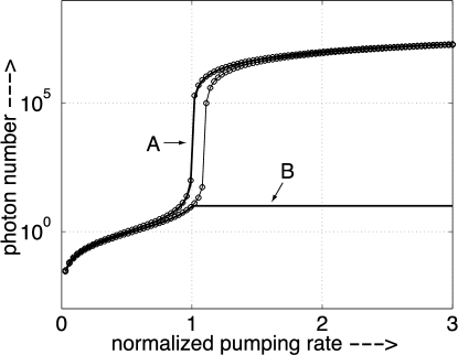
Figure 7: Photon numbers $n_{A}$ and $n_{B}$ versus normalized pumping rate $r$ when the optical mode intensities $|u_{A}|^{2}$ and $|u_{B}|^{2}$ are (a) constant in space and (b) have spatial variation. Mode $B$ cannot lase when the mode intensities are uniform in (a). Spatial variations in the mode intensities allow mode $B$ to lase in (b).

Figure 7 shows the photon numbers $n_{A}$ and $n_{B}$ for two modes competing on a homogeneous line. In Fig. 7(a) the optical mode intensities are constant, so that $|u_{A}|^{2}=|u_{B}|^{2}=1/(A_{L}L)$ (as we implicitly assumed for the gas laser of section 2). Figure 7(a) therefore mimics the case where spatial variations in the laser are negligible. Two other cases where we can neglect spatial variation of the mode intensities are in a ring laser or in a semiconductor laser with rapid electron diffusion. In Fig. 7(a) the photon number $n_{B}$ in mode $B$ is fixed whenever mode $A$ begins lasing. The solution of Eqs. (27)-(28) therefore reproduces lasing on a homogeneous line whenever the optical mode intensities $|u_{A}|^{2}$ and $|u_{B}|^{2}$ are constant. We let the optical mode intensities vary in space in Fig. 7(b), where we have taken the lowest two longitudinal cavity modes ($A=1$ and $B=2$). Mode $B$ can indeed begin lasing in Fig. 7(b), but requires a higher pumping rate than for two independent lasers on the same optical line. We have chosen parameters $z=1.1$ and $p=10^{7}$ in Fig. 7. The circles in Fig. 7 show the solutions from Eqs. (8)-(9) for two independent single mode lasers.

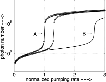
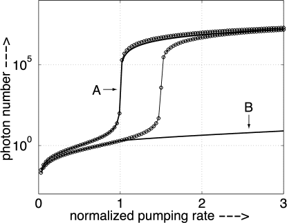
Figure 8: Increasing the ratio of the optical rate constants from $z=\tilde{K}_{A}/\tilde{K}_{B}=1.1$ in Figure 7 to (a) $z=1.3$ and (b) $z=1.5$ increases the threshold current required for mode $B$ to lase. Spatial variations in the optical intensities become less relevant when the optical rate constant for mode $B$ becomes too small.

Spatial vatiations in the optical mode intensities $|u_{A}|^{2}$ and $|u_{B}|^{2}$ become less relevant when the optical rate constant $\tilde{K}_{B}$ becomes small. The ratio of the rate constants $z=\tilde{K}_{A}/\tilde{K}_{B}$ in Fig. 7 is $z=1.1$. We increase $z$ in Fig. 8 to (a) $z=1.3$ and (b) $z=1.5$, raising the threshold current required for mode $B$ to lase. For the parameter $z=1.5$ in Fig. 8(b), mode $B$ no longer lases for the range of pumping currents shown $(0\leq r\leq 3)$. Although spatial variations in the optical mode intensities are still present in Fig. 8, they become less relevant when the optical coupling constant $\tilde{K}_{B}$ for mode $B$ is too weak.

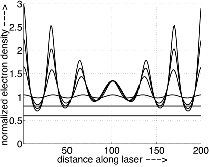
Figure 9: (a) Photon numbers and (b) electron density $\rho(x)$ for two higher lying longitudinal modes $A=6$ and $B=7$. The photon numbers versus pumping in (a) depend only weakly on the number of half wavelengths in the laser cavity. Spatial holes are burned into the electron density $\rho(x)$ in (b), due both to the mirrors and the oscillating optical mode intensities.

Figure 9(a) shows the photon numbers $n_{A}$ and $n_{B}$ versus pumping and for two higher lying longitudinal modes having $A=6$ and $B=7$. The photon numbers $n_{A}$ and $n_{B}$ in Fig. 9(a) are essentially unchanged from those for the two lowest cavity modes having $A=1$ and $B=2$ in Fig. 7(b). Figure 9 and Fig. 7 use the same parameters, namely $z=1.1$ and $p=10^{7}$. The photon numbers $n_{A}$ and $n_{B}$ versus pumping therefore have little (if any) dependence on the number of half wavelengths in the cavity. The weak dependence of Fig. 7(a) on the number of half wavelengths (where $A-B=1$) is because the fraction of the gain media where $|u_{B}|^{2}\geq|u_{A}|^{2}$ is essentially independent of the number of half wavelengths in the cavity, as can be checked numerically.

Spatial holes are burned into the electron density $\rho(x)$ in Fig. 9(b), especially when mode $B$ begins lasing. Figure 9(b) shows the electron density $\rho(x)$ inside the active laser medium for different pumping rates $r$. Because the mode intensities have a node at the mirrors and there is no electron diffusion, the pumping rates can be read directly from the normalized density axis at the mirrors (points $l=0$ and $l=200$) in Fig. 9(b). The normalized pumping rates in Fig. 7(b) are $r=0.6,0.8,1.05,1.65,2.25,3.0$. The electron density $\rho(x)$ is essentially constant for pumping rates below threshold ($r=0.6,0.8$) in Fig. 7(b). There is a small variation in electron density for pumping rates below threshold, which is invisible on the scale in Fig. 9(b). Above threshold the variation in electron density becomes quite pronounced, especially when mode $B$ begins lasing ($r=1.65,2.25,3.0$). The growth of electron density $\rho(x)$ as we move from the center of the gain media towards the mirrors is due to our neglect of diffusion. Since the optical mode intensites $|u_{A}|^{2}$ and $|u_{B}|^{2}$ have a node at the mirrors, a large spatial hole is also burned into the main body of the laser. Smaller spatial holes arising from the oscillating optical mode intensities produce oscillations in the electron density.

3.2 Fast Diffusion

When we include diffusion $(D\neq 0)$, we can no longer solve Eq. (19) directly for the density $\rho(x)$. Instead we discretize the active lasing medium, taking lattice points $x_{l}=la$. Here $a$ is the lattice spacing and $0\leq l\leq l_{max}$, with $L_{a}=l_{max}a$ the length of the active medium. With this lattice Eq. (19) reads

$$\frac{d}{dt}\left[\begin{array}[]{c}\vdots\\ \rho_{l-1}\\ \rho_{l}\\ \rho_{l+1}\\ \vdots\end{array}\right]=\left[\begin{array}[]{ccccc}\ddots&\vdots&\vdots&\vdots&\cdots\\ t&-2t+w_{l-1}&t&0&0\\ 0&t&-2t+w_{l}&t&0\\ 0&0&t&-2t+w_{l+1}&t\\ \cdots&\vdots&\vdots&\vdots&\ddots\\ \end{array}\right]\left[\begin{array}[]{c}\vdots\\ \rho_{l-1}\\ \rho_{l}\\ \rho_{l+1}\\ \vdots\end{array}\right]+\left[\begin{array}[]{c}\vdots\\ R_{l-1}\\ R_{l}\\ R_{l+1}\\ \vdots\end{array}\right].$$ (32)

Here $t=D/a^{2}$ is the diffusion rate and

$$-w_{l}=\tilde{K}_{A}V_{L}n_{A}|u_{A}(x_{l})|^{2}+\tilde{K}_{B}V_{L}n_{B}|u_{B}(x_{l})|^{2}+\tilde{A}.$$ (33)

Given an initial guess for the photon numbers $n_{A}$ and $n_{B}$, we can invert Eq. (32) for the density $\rho(x)$ in steady state. Taking a hypothetical five point lattice we have

$$-\left[\begin{array}[]{c}\rho_{0}\\ \rho_{1}\\ \rho_{2}\\ \rho_{3}\\ \rho_{4}\end{array}\right]=\left[\begin{array}[]{ccccc}-t+w_{0}&t&0&0&0\\ t&-2t+w_{1}&t&0&0\\ 0&t&-2t+w_{2}&t&0\\ 0&0&t&-2t+w_{3}&t\\ 0&0&0&t&-t+w_{4}\\ \end{array}\right]^{-1}\left[\begin{array}[]{c}R_{0}\\ R_{1}\\ R_{2}\\ R_{3}\\ R_{4}\end{array}\right].$$ (34)

We use zero derivitive boundary conditions to truncate the matrix in Eq. (34). After solving Eq. (34) numerically for $\rho_{l}$, we can substitute this density back into Eqs. (20)-(21) to generate updated photon numbers $n_{A}$ and $n_{B}$ in steady state. We move from the $m$th to the $(m+1)$st iteration for the photon numbers by

$$n_{A}(m+1)=(n_{A}(m)+1)\int_{a}\frac{[\tilde{K}_{A}V_{L}]}{\gamma_{A}}|u_{A}|^{2}\rho dV,$$ (35)

and

$$n_{B}(m+1)=(n_{B}(m)+1)\int_{a}\frac{[\tilde{K}_{B}V_{L}]}{\gamma_{B}}|u_{B}|^{2}\rho dV.$$ (36)

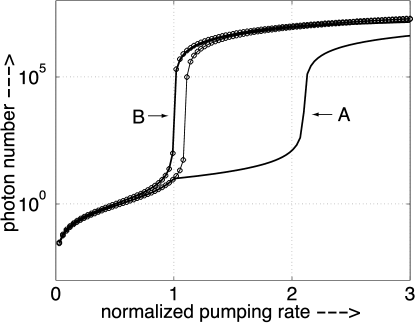
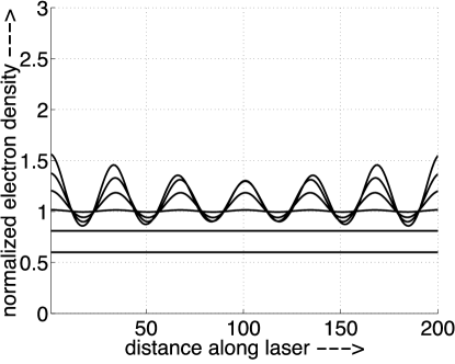
Figure 10: (a) Photon numbers and (b) electron density $\rho(x)$ when the electron diffusion constant is $D=(9/400)\lambda^{2}\tilde{A}$. Adding some electron diffusion has raised the threshold current for mode $B$ and reduced spatial hole burning effects due to the mirrors.

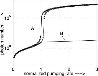
Figure 11: (a) Photon numbers and (b) electron density $\rho(x)$ when the electron diffusion constant is $D=(45/400)\lambda^{2}\tilde{A}$. The diffusion constant is now large enough that mirror effects are negligible. The electron density oscillates essentially periodically and the photon number in mode $B$ is essentially constant above threshold.

Figures 10 and 11 show the effects of adding electron diffusion to the photon numbers and electron density in Fig. 9. In Figs. 10-11 the number of half wavelengths in the cavity are $A=6$ and $B=7$ with a ratio of optical rate constants $z=\tilde{K}_{A}/\tilde{K}_{B}=1.1$, the same parameters as in Fig. 9. Figure 10 uses a diffusion constant $D=100a^{2}\tilde{A}$ with $L=200a$ ($t=100p$ with $l_{max}=200$), while Fig. 11 uses a larger diffusion constant $D=500a^{2}\tilde{A}$ with $L=200a$ ($t=500p$ with $l_{max}=200$). Since the cavity is six half wavelengths long ($L=6\lambda/2$), we have $D=(9/400)\lambda^{2}\tilde{A}$ in Fig. 10 and $D=(45/400)\lambda^{2}\tilde{A}$ in Fig. 11. These values for the diffusion constant are in good agreement with our order of magnitude estimate for when diffusion should affect the laser output characteristics.

Adding electron diffusion raises the threshold current required for mode $B$ to lase, as can be seen in Figs. 10(a) and 11(a). The larger the diffusion constant, the greater is the threshold current required for mode $B$ to begin lasing. Diffusion also reduces the spatial hole burning effects due to the mirrors, leaving only the smaller spatial holes due to the difference in the number of half wavelengths in the cavity between modes $A$ and $B$. Some overall gradients are still visible in the electron density in Fig. 10(b), while in Fig. 11(b) the overall average electron density density is essential uniform (mirror effects are negligible). Fig. 11(b) resembles the picture of electron density used to illustrate the effects of spatial hole burning in the laser in Ref. [2].

4 Conclusions

We have generalized the laser rate equations in Refs. [2, 3] both electron scattering between the different lasing levels to describe spectral hole burning effects in gas lasers. In order to model spatial hole burning effects present in semiconductor lasers, and guided by Ref. [4], we then further generalized the rate equation model to include the effects of spatially varying optical mode intensities in the laser.

In order for multiple frequencies to lase simultaneously, either the energy spectrum or spatial variation of the optical gain must be broken up into many independent (single moded) lasers. Electron equilibration (scattering rate) is slow in gas lasers, and this allows the energy spectrum to be broken up into many independent frequency ranges. An order or magnitude estimate for single mode laser operation to occur in gas lasers is that the scattering rate between electrons in the different energy ranges must exceed the spontaneous emission rate ($s\gg A$). For semiconductor lasers the electron diffusion is slow, and the gain media can be viewed as many independent lasers at each point in space. Due to spatial variations in the optical mode intensities, different lasing modes will be favored at each point in space. Since the regions where different modes dominate lasing are spatially separated by about one quarter wavelength, we need the diffusion constant to exceed $D\gg\lambda^{2}A/16$ for single moded operation in semiconductor lasers. Numerical simulations given in this paper agree with these two order of magnitude estimates for the transition from single to multiple moded laser operation.

Finally, we can summarize some general (and well known) conclusions about single versus multiple moded laser operation. Firstly, all lasers are single moded for some range of pumping rates near threshold. The range of pumping rates for single moded operation is larger for more scattering between electronic states and for faster electronic diffusion. But a range of pumping rates for single moded operation nonetheless exists no matter how weak the equilibration or how slow the electronic diffusion (unless two degenerate states are lasing). Secondly, all lasers become multi-moded when pumped hard enough (unless the gain medium is first destroyed by too high of a pumping rate). Finally, bad economic analogies do not describe laser mode competition. Statements such as ’Laser mode competition is just like life. The rich get richer and the poor get poorer.’ are clearly incorrect. Even as the photon number in mode $A$ increases, the worst that can happen is that the photon number in mode $B$ remains constant. Mode $B$ can also begin lasing (become an economic success) either by electrons scattering from mode $A$ (working in a supporting industry often created by a competitor) or by specializing its spatial mode pattern to take advantage of optical gain inaccessible to $A$ (working in another area of the economy to exploit talents and resources unavailable to a competitor).

References

[1]D. Ross, Light Amplifiers and Oscillators, (Academic Press,
New York, 1969).
[2]A.E. Siegman, An Introduction to Masers and Lasers,
(McGraw-Hill, New York, 1971).
[3]A.E. Siegman, Lasers, (McGraw-Hill, New York, 1986).
[4]O. Svelto, Principles of Lasers, (Plenum Press, New York, 1998).
[5]R. Loudon, The Quantum Theory of Light,
(Oxford University Press, Oxford, 1983).
[6]L.W. Casperson, J. Appl. Phys., 46 , 5194 (1975).