The Richardson’s Law in Large-Eddy Simulations of Boundary Layer flows

Abstract

Relative dispersion in a neutrally stratified planetary boundary layer (PBL) is investigated by means of Large-Eddy Simulations (LES). Despite the small extension of the inertial range of scales in the simulated PBL, our Lagrangian statistics turns out to be compatible with the Richardson $t^{3}$ law for the average of square particle separation. This emerges from the application of nonstandard methods of analysis through which a precise measure of the Richardson constant was also possible. Its values is estimated as $C_{2}\sim 0.5$ in close agreement with recent experiments and three-dimensional direct numerical simulations.

1 Introduction

One of the most striking features of a turbulent planetary boundary layer (PBL) is the presence of a wide range of active length scales. They range from the smallest dynamically active scales of the order of millimeters (the so-called Kolmogorov scale), below which diffusive effects are dominant, to the largest scales of the order of ten kilometers. Such a large range of excited scales are essentially a continuum and the distribution of energy scale-by-scale is controlled by the famous Kolmogorov’s 1941 prediction (see Frisch, 1995 for a modern presentation).
One of the most powerful concepts which highlighted the dynamical role of the active scales in the atmosphere was due to Richardson (1926). He introduced in his pioneering work the concept of turbulent relative dispersion (see Sawford, 2001 for a recent review) with the aim of investigating the large variations of atmospheric turbulent diffusion when observed at different spatial scales.
In his work, Richardson proposed a diffusion equation for the probability density function, $p({\mbox{\boldmath$r$}},t)$, of pair separation. Assuming isotropy such an equation can be cast into the form

$$\frac{\partial p({\mbox{\boldmath$r$}},t)}{\partial t}=\frac{1}{r^{2}}\frac{\partial}{\partial r}\left[r^{2}D(r)\frac{\partial p(\mbox{\boldmath$r$},t)}{\partial r}\right]$$ (1)

where the scale-dependent eddy-diffusivity $D(r)$ accounts for the enormous increase in observed values of the turbulent diffusivity in the atmosphere.
The famous scaling law $D(r)\propto r^{4/3}$ was obtained by Richardson (1926) from experimental data. From the expression of $D(r)$ as function of $r$ and exploiting Eq. (1) the well known non-Gaussian distribution

$$p({\mbox{\boldmath$r$}},t)\propto t^{-9/2}\exp\left(-Cr^{2/3}/t\right)$$ (2)

is easily obtained.
This equation implies that the mean square particle separation grows as

$$R^{2}(t)\equiv\langle r^{2}(t)\rangle=C_{2}\epsilon t^{3}$$ (3)

which is the celebrated Richardson’s “$t^{3}$” law for the pair dispersion. Here $C_{2}$ is the so-called Richardson constant and $\epsilon$ is the mean energy dissipation.
Despite the fact that the Richardson’s law has been proposed since a long time, there is still a large uncertainty on the value of $C_{2}$. Some authors have found $C_{2}$ ranging from $\sim 10^{-2}$ to $\sim 10^{-1}$ in kinematic simulations (see, for example, Elliot and Majda, 1996; Fung and Vassilicos, 1998), although for kinematic models an energy flux $\epsilon$ can hardly be defined. On the other hand, a value $C_{2}\sim O(1)$ (and even larger) follows from closure predictions (Monin and Yaglom, 1975). More recently, both an experimental investigation (Ott and Mann, 2000) and accurate three-dimensional direct numerical simulations (DNS) (Boffetta and Sokolov, 2002) give a strong support for the value $C_{2}\sim 0.5$.
The main limitation of the state-of-the-art three-dimensional DNS is that the achieved Reynolds numbers are still far from those characterizing the so-called fully developed turbulence regime, that is the realm of the Richardson’s (1926) theory. Moreover, initial and boundary conditions assumed in the most advanced DNS are, however, quite idealized and do not match those characterizing a turbulent PBL, the main concern of the present paper.
For all these reasons we have decided to focus our attention on Large-Eddy Simulations (LES) of a neutrally stratified PBL and address the issue related to the determination of the Richardson constant $C_{2}$. The main advantage of this strategy is that it permits to achieve very high Reynolds numbers and, at the same time, it properly reproduces the dynamical features observed in the PBL.
It is worth anticipating that the naive approach which should lead to the determination of $C_{2}$ by looking at the behavior of $R^{2}(t)$ versus the time $t$ is extremely sensitive to the initial pair separations and thus gives estimations of the Richardson’s constant which appear quite questionable (see Fig. 3). This is simply due to the fact that, in realistic situations like the one we consider, the inertial range of scales is quite narrow and, consequently, there is no room for a genuine $t^{3}$ regime to appear (see Boffetta et al., 2000 for general considerations on this important point).
This fact motivated us to apply a recently established ‘nonstandard’ analysis technique (the so-called FSLE approach, Boffetta et al., 2000) to isolate a clear Richardson regime and thus to provide a reliable and systematic (that is independent from initial pair separations) measure for $C_{2}$. This is the main aim of our paper.

2 The LES strategy

In a LES strategy the large scale motion (that is motion associated to the largest turbulent eddies) is explicitly solved while the smallest scales (typically in the inertial range of scales) are described in a statistical consistent way (that is parameterized in terms of the resolved, large scale, velocity and temperature fields). This is done by filtering the governing equations for velocity and potential temperature by means of a filter operator. Applied, for example, to the $i$th-component of the velocity field, $u_{i}$, ($u_{1}=u$, $u_{2}=v$, $u_{3}=w$), the filter is defined by the convolution:

$$\overline{u}_{i}({\mbox{\boldmath$x$}})=\int u_{i}({\mbox{\boldmath$x$}}^{\prime})G({\mbox{\boldmath$x$}}-{\mbox{\boldmath$x$}}^{\prime})d{\mbox{\boldmath$x$}}^{\prime}$$ (4)

where $\overline{u}_{i}$ is the filtered field and $G({\mbox{\boldmath$x$}})$ is a three-dimensional filter function. The field component $u_{i}$ can be thus decomposed as

$$u_{i}=\overline{u}_{i}+{u}_{i}^{\prime\prime}$$ (5)

and similarly for the temperature field. In our model, the equation for the latter field is coupled to the Navier–Stokes equation via the Boussinesq term.
Applying the filter operator both to the Navier–Stokes equation and to the equation for the potential temperature, and exploiting the decomposition (5) (and the analogous for the temperature field) in the advection terms one obtains the corresponding filtered equations:

$$\frac{\partial\overline{u}_{i}}{\partial t} = -\frac{\partial\overline{\overline{u}_{i}\overline{u}_{j}}}{\partial x_{j}}-\frac{\partial\tau_{ij}^{(u)}}{\partial x_{j}}-\frac{1}{\rho}\frac{\partial\overline{p}}{\partial x_{i}}+g_{i}\frac{\overline{\theta}}{\theta_{0}}\delta_{i3}-f\epsilon_{ij3}\overline{u}_{j}+\nu\nabla^{2}\overline{u}_{i}$$ (6)

$$\frac{\partial\overline{u}_{i}}{\partial x_{i}} = 0$$ (7)

$$\frac{\partial\overline{\theta}}{\partial t} = -\frac{\partial\overline{\overline{u_{j}}\overline{\theta}}}{\partial x_{j}}-\frac{\partial\tau_{j}^{(\theta)}}{\partial x_{j}}+\kappa\nabla^{2}\overline{\theta}$$ (8)

where $\rho$ is the air density, $p$ is the pressure, $f$ is the Coriolis parameter, $\nu$ is the molecular viscosity, $\kappa$ is the thermal molecular diffusivity, $g_{i}\frac{\theta}{\theta_{0}}\delta_{i3}$ is the buoyancy term and $\theta_{0}$ is a reference temperature profile. The quantities to be parametrized in terms of large scale fields are

$$\tau_{ij}^{(u)}=\overline{\overline{u}_{i}u^{\prime\prime}_{j}}+\overline{u^{\prime\prime}_{i}\overline{u}_{j}}+\overline{u^{\prime\prime}_{i}u^{\prime\prime}_{j}};\qquad\tau_{j}^{(\theta)}=\overline{\overline{\theta}u^{\prime\prime}_{j}}+\overline{\theta^{\prime\prime}\overline{u}_{j}}+\overline{\theta^{\prime\prime}u^{\prime\prime}_{j}},$$ (9)

that represent the subgrid scale (SGS) fluxes of momentum and heat, respectively.

Table 1: The relevant parameters characterizing the simulated PBL. In this table, $L_{x}$, $L_{y}$ and $L_{z}$ are the domain extension along the directions $x$, $y$ and $z$, respectively; $Q_{*}$ is the heat flux from the bottom boundary; $U_{g}$ is the geostrophic wind; $z_{i}$ is the mixed layer depth, $u_{*}$ is the friction velocity and $\tau_{*}\equiv z_{i}/u_{*}$ is the turnover time;

parameter		value
$L_{x}$, $L_{y}$	[km]	2
$L_{z}$	[km]	1
$Q_{*}$	[m K s-1]	0
$U_{g}$	[m s-1]	15
$z_{i}$	[m]	461
$u_{*}$	[ms-1]	0.7
$\tau_{*}$	[s]	674

In our model:

$$\tau^{(u)}_{ij}=-2K_{M}\left(\partial_{i}\overline{u}_{j}+\partial_{j}\overline{u}_{i})\right)$$ (10)

$$\tau^{(\theta)}_{i}=-K_{H}\partial_{i}\overline{\theta}$$ (11)

$K_{M}$ and $K_{H}$ being the SGS eddy coefficients for momentum and heat, respectively.
The above two eddy coefficients are related to the velocity scale $\overline{e^{\prime}}^{1/2}$, $\overline{e^{\prime}}$ being the SGS turbulence energy the equation of which is solved in our LES model (Moeng, 1984), and to the length scale $l\equiv(\Delta x\Delta y\Delta z)^{1/3}$ (valid for neutrally stratified cases) $\Delta x$, $\Delta y$, and $\Delta z$ being the grid mesh spacing in $x$, $y$ and $z$. Namely:

$$K_{M}=0.1\;l\;\overline{e^{\prime}}^{1/2}$$ (12)

$$K_{H}=3K_{M}.$$ (13)

Details on the LES model we used in our study can be found in Moeng, 1984 and in Sullivan et al., 1994. Such a model has been widely used and tested to investigate basic research problems in the framework of boundary layer flows (see, for example, Antonelli et al., 2003 and Moeng and Sullivan, 1994 among the others).

3 The simulated PBL

In order to obtain a stationary PBL we advanced in time our LES code for around six large-eddy turnover times, $\tau_{*}$, with a spatial resolution of $128^{3}$ grid points. This time will be the starting point for the successive Lagrangian analysis (see next section).
The relevant parameters characterizing our simulated PBL are listed in Table 1 at $t=6\;\tau_{*}$. At the same instant, we show in Fig. 1 the horizontally averaged vertical profile of the velocity components $u$, $v$. The average of the vertical component is not shown, the latter being very close to zero. We can observe the presence of a rather well mixed region which extends from $z\sim 0.2\;z_{i}$ to $z\sim z_{i}$.

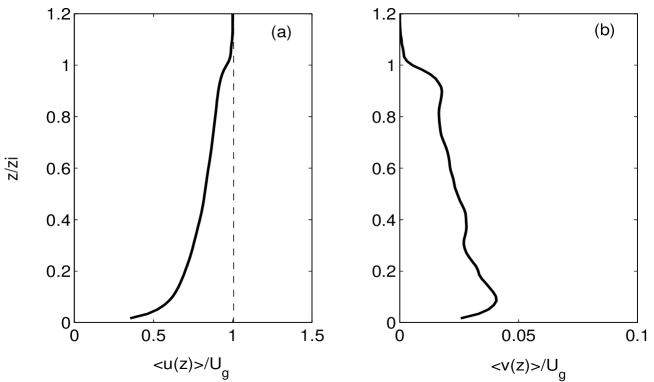
Figure 1: The horizontally averaged velocity profiles. (a): stream-wise $u$-component, (b) span-wise $v$-component.

The energy spectra for the three velocity components are reported in Fig. 2. Dashed lines are relative to the Kolmogorov (K41) prediction $E(k)\propto k^{-5/3}$. Although the inertial range of scale appears quite narrow, data are compatible with the K41 prediction.

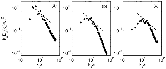
Figure 2: Energy spectra for the three components of the velocity field. (a): stream-wise, (b) span-wise, (c) vertical. The dashed lines correspond to the K41 prediction.

4 Lagrangian simulations

In order to investigate the statistics of pair dispersion, from the time $t=6\;\tau_{*}$ (corresponding to the PBL stationary state) we integrated, in parallel to the LES, the equation for the passive tracer trajectories defined by the equation

$$\dot{\mbox{\boldmath$x$}}(t)={\mbox{\boldmath$u$}}({\mbox{\boldmath$x$}}(t),t).$$ (14)

We performed a single long run where the evolution of 20000 pairs has been followed starting from two different initial separations: $R(0)=\Delta x$ and $R(0)=2\Delta x$, $\Delta x$ being the grid mesh spacing whose value is 15.6 $m$. Trajectories have been integrated for a time of the order of 5000 $s$ with a time step of around 1 $s$, the same used to advance in time the LES.
At the initial time, pairs are uniformly distributed on a horizontal plane placed at the elevation $z_{i}/2$. Reflection has been assumed both at the capping inversion (at the elevation $z_{i}$) and at the bottom boundary.
For testing purposes, a second run (again started from $t=6\;\tau_{*}$) with a smaller number of pairs (5000) has been performed. No significant differences in the Lagrangian statistics have been however observed. The same conclusion has been obtained for a second test where the LES spatial resolution has been lowered to $96^{3}$ grid points. For a comparison see Figs. 3 and 4.
The velocity field necessary to integrate (14) has been obtained by a bilinear interpolation from the eight nearest grid points on which the velocity field produced by the LES is defined.
In this preliminary investigation, we did not use any sub-grid model describing the Lagrangian contribution arising from the motion on scales smaller than the grid mesh spacing.

4.1 Pair dispersion statistics

In Fig. 3 we show the second moment of relative dispersion $R^{2}(t)$ for the two initial separations. Heavy dashed line represents the expected Richardson’s law, which is however not compatible with our data for the largest initial separation $2\Delta x$. We can also notice how the $R^{2}(t)$ curve becomes flatter for larger separations. The same dependence has been observed by Boffetta and Celani (2000) for pair dispersion in two-dimensional turbulence.

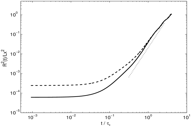
Figure 3: The behavior of the (dimensionless) mean square relative dispersion vs the (dimensionless) time. Full line: the initial separation is $\Delta x$; Dashed-line: the initial separation is $2\Delta x$. Dotted line is relative to the $t^{3}$ Richardson’s law.

The fact that our data do not fit the Richardson law, for generic initial pair separations, is simply explained as a consequence of finite size effects (in space and in time) of our system. Indeed, it is clear that, unless $t$ is large enough that all particle pairs have “forgotten” their initial conditions, the average will be biased. This is why we observe a consistent flattening of $R^{2}(t)$ at small times. Such regime is a crossover from initial conditions to the Richardson regime. From Fig. 3 we can see that the extension of such crossover increases as the initial separation increases.
Unfortunately, we cannot augment the time $t$ too much because of the reduced extension of our inertial range (see Fig. 2). To overcome this problem, and thus to allow a systematic estimation of the Richardson constant which does not depend on the choice of the initial pair separation, we use an alternative approach based on statistics at fixed scale (Boffetta et al., 2000). This is the subject of the next subsection.

4.2 Fixed-scale statistics

The characterization of transport properties in multi-scale systems, such as models of turbulent fluids, is a delicate task, especially when exponents of scaling laws and/or universal constants are to be measured from Lagrangian statistics. Additional difficulties arise in all cases where the standard asymptotic quantities, for example the diffusion coefficients, cannot be computed correctly, for limitations due essentially to the finite size of the domain and to finite spatio-temporal resolution of the data. As we have seen in the previous subsection for the LES trajectories, the mean square relative dispersion, seen as a function of time, is generally affected by overlap effects between different regimes. We therefore use a mathematical tool known as Finite-Scale Lyapunov Exponent, briefly FSLE, a technique based on exit-time statistics at fixed scale of trajectory separation, formerly introduced in the framework of chaotic dynamical systems theory (for a review see Boffetta et al., 2000, and references therein).
A dynamical system consists, basically, of a $N$-dimensional state vector $x$, having a set of $N$ observables as components evolving in the so-called phase space, and of a $N$-dimensional evolution operator $F$, related by a first-order ordinary differential equations system:

$${\dot{\mbox{\boldmath$x$}}}(t)={\mbox{\boldmath$F$}}[{\mbox{\boldmath$x$}}].$$ (15)

If $F$ is nonlinear, the system (15) can have chaotic solutions, that is limited predictability, for which case an infinitesimally small error $\delta{\mbox{\boldmath$x$}}$ on a trajectory $x$ is exponentially amplified in time:

$$\delta{\mbox{\boldmath$x$}}(t)\sim\delta{\mbox{\boldmath$x$}}(0)\exp{\lambda t}$$ (16)

with a (mean) growth rate $\lambda$ known as Maximum Lyapunov Exponent (MLE). The FSLE is based on the idea of characterizing the growth rate of a trajectory perturbation in the whole range of scales from infinitesimal to macroscopic sizes. In the Lagrangian description of fluid motion, the vector $x$ is the tracer trajectory, the operator $F$ is the velocity field, and the error $\delta{\mbox{\boldmath$x$}}$ is the distance between two trajectories. It is therefore straightforward to consider the relative dispersion of Lagrangian trajectories as a problem of finite-error predictability.

At this regard, the FSLE analysis has been applied in a number of recent works as diagnostics of transport properties in geophysical systems (see, for example, Lacorata et al., 2001; Joseph and Legras, 2002; LaCasce and Ohlmann, 2003).

The procedure to define the FSLE is the following. Let $r=|\delta{\mbox{\boldmath$x$}}|$ be the distance between two trajectories. Given a series of $N$ spatial scales, or thresholds, $\delta_{1},\delta_{2},\cdots,\delta_{N}$ have been properly chosen such that $\delta_{i+1}=\rho\cdot\delta_{i}$, for $=1,\cdots,N-1$ and with $\rho>1$, the FSLE is defined as

$$\lambda(\delta)={{\rm ln}\,\rho\over\langle T(\delta)\rangle}$$ (17)

where $\langle T(\delta)\rangle$ is the mean exit-time of $r$ from the threshold $\delta=\delta_{i}$, in other words the mean time taken for $r$ to grow from $\delta$ to $\rho\delta$. The FSLE depends very weakly on $\rho$ if $\rho$ is chosen not much larger than $1$. The factor $\rho$ cannot be arbitrarily close to $1$ because of finite-resolution problems and, on the other hand, must be kept sufficiently small in order to avoid contamination effects between different scales of motion. In our simulations we have fixed $\rho=\sqrt{2}$. For infinitesimal $\delta$, the FSLE coincides with the MLE. In general, for finite $\delta$, the FSLE is expected to follow a power law of the type:

$$\lambda(\delta)\sim\delta^{-2/\gamma}$$ (18)

where the value of $\gamma$ defines the dispersion regime at scale $\delta$, for example: $\gamma=3$ refers to Richardson diffusion within the turbulence inertial range; $\gamma=1$ corresponds to standard diffusion, that is large-scale uncorrelated spreading of particles. These scaling laws can be explained by dimensional argument: if the scaling law of the relative dispersion in time is of the form $r^{2}(t)\sim t^{\gamma}$, the inverse of time as function of space gives the corresponding scaling (18) of the FSLE. In our case, indeed, we seek for a power law related to Richardson diffusion, inside the inertial range of the LES:

$$\lambda(\delta)=\alpha\delta^{-2/3}$$ (19)

where $\alpha$ is a constant depending on the details of the numerical experiment. The corresponding mean square relative separation is expected to follow Eq. (3). A formula can be derived, which relates the FSLE to the Richardson’s constant (Boffetta and Sokoloff, 2002):

$$C_{2}=\beta{\alpha^{3}\over\epsilon}\left({\rho^{2/3}-1\over\rho^{2/3}{\rm ln}\,\rho}\right)^{3}$$ (20)

where $\beta$ is a numerical coefficient equal to $1.75$, $\epsilon$ is the energy dissipation measured from the LES and $\alpha$ comes from the best fit of Eq. (19) to the data. Information about the existence of the inertial range is also given by a quantity related to the FSLE, the mean relative Lagrangian velocity at fixed scale that we indicate with

$$\nu(\delta)=[\langle\delta{\mbox{\boldmath$v$}}(\delta)^{2}\rangle]^{1/2}$$ (21)

where

$$\delta{\mbox{\boldmath$v$}}(\delta)^{2}=({\dot{\mbox{\boldmath$x$}}^{(1)}}-{\dot{\mbox{\boldmath$x$}}^{(2)}})^{2}$$ (22)

is the square (Lagrangian) velocity difference between two trajectories, ${\mbox{\boldmath$x$}}^{(1)}$ and ${\mbox{\boldmath$x$}}^{(2)}$, on scale $\delta$, that is for $|{\mbox{\boldmath$x$}}^{(1)}-{\mbox{\boldmath$x$}}^{(2)}|=\delta$. The quantity $\nu(\delta)/\delta$ is dimensionally equivalent to $\lambda(\delta)$, and, in conditions of sufficient isotropy, it represents the spectrum of the relative dispersion rate in real space. A scaling law of the type

$${\nu(\delta)\over\delta}\sim\delta^{-2/3}$$ (23)

is compatible with the FSLE inside the inertial range and therefore with the expected behavior of the turbulent velocity difference as function of the scale. In Fig. 4(a) we can see, indeed, that the FSLE measured from the LES data follows the behavior of Eq. (19), from the scale of the spatial resolution to about the size of the domain. From the fit we extract the coefficient $\alpha=0.1\;m^{2/3}t^{-1}$. The energy dissipation measured from the LES is $\epsilon=6\cdot 10^{-4}\;m^{2}t^{-3}$. The formula of Eq. (20) gives a measure of the Richardson’s constant $C_{2}\sim 0.5$, affected, at most, by an estimated error of $\pm 0.2$. In Fig. 4(b) we see, also, that $\nu(\delta)/\delta$ has been found very close to the behavior predicted by Eq. (23).

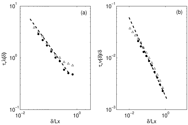
Figure 4: a) FSLE at two different resolutions. Triangles: $128^{3}$ grid points; Circles: $96^{3}$ grid points. The dashed line corresponds to $\alpha\delta^{-2/3}$ with $\alpha=0.1$ $m^{2}t^{-3}$. b) the same as in a) but for the relative velocity. The dashed line has slope $-2/3$.

Variations within the error bars are observed by varying the spatial resolution from $128^{3}$ grid points (triangles in Fig. 4) to $96^{3}$ grid points (circles).

5 Conclusions and perspectives

We have investigated the problem of relative dispersion in a neutrally stratified planetary boundary layer simulated by means of Large-Eddy Simulations. In particular, our attention has been focused on the possible emergence of the celebrated Richardson’s law ruling the separation in time of particle pairs.
The difficulties in observing such behavior in a realistic PBL mainly rely on the fact that it is hard to obtain a PBL with a sufficiently extended inertial range of scales. For this reason, standard techniques to isolate the Richardson’s law and the relative constant turn out to be inconclusive, the results being strongly dependent, for instance, on the choice of the initial pair separations. To overcome this problem, we have applied, for the first time in the context of boundary layer physics, a recently established technique coming from the study of dynamical systems. As a result, a clean region of scaling showing the occurrence of the Richardson law has been observed and an accurate, systematic, measure of the Richardson constant became possible. Its value is $C_{2}=(0.5\pm 0.2)$, where the error bar has been determined in a very conservative way. Such estimation is compatible with the one obtained from Fig. 3 in the case of initial pair separation equal to $\Delta x$. The important point is that the new strategy gives a result that, by construction, does not depend on the initial pair separations. As already emphasized this is not the case for the standard approach.

Clearly, our study is not the end of the story. The following points appear to be worth investigating in a next future.
The first point is related to the fact that in our simulations we did not use any sub-grid model for the unresolved Lagrangian motions. The main expected advantage of SGS Lagrangian parameterizations is to allow the choice of initial pair separations smaller than the grid mesh spacing, a fact that would cause a reduction of the crossover from initial conditions to the genuine $t^{3}$ law. The investigation of this important point is left for future research.
Another point is related to the investigation of the probability density function (pdf) of pair separation. In the present study, we have focused on the sole second moment of this pdf. There are, indeed, several solutions for the diffusion equation (1) all giving pdfs compatible with the $t^{3}$ law. The solution for the pdf essentially depends on the choice for the eddy-diffusivity field, $D(r)$. The answer to this question concerns applicative studies related, for example, to pollutant dispersion because of the importance of correctly describing the occurrence of extreme, potentially dangerous, events.
Finally, it is also interesting to investigate whether or not the Richardson law rules the behavior of pair separations also in buoyancy-dominated boundary layers. In this case, the role of buoyancy could modify the expression for the eddy-diffusivity field, $D(r)$, thus giving rise to an essentially new regime which is however up to now totally unexplored.

Aacknowledgements

This work has been partially supported by Cofin 2001, prot. 2001023848 (A.M.) and by CNPq 202585/02 (E.P.M.F.). We acknowledge useful discussions with Guido Boffetta and Brian Sawford.

References

- [1] Antonelli, M., A. Mazzino and U. Rizza. Statistics of temperature fluctuations in a buoyancy dominated boundary layer flow simulated by a Large-eddy simulation model. J. Atmos. Sci., 60:215–224, 2003.
- [2] Boffetta, G., A. Celani. Pair dispersion in turbulence. Physica A, 280:1–9, 2000.
- [3] Boffetta G. and I.M. Sokolov. Relative dispersion in fully developed turbulence: the Richardson’s law and intermittency corrections. Phys. Rev. Lett, 88:094501, 2002
- [4] Boffetta, G., A. Celani, M. Cencini, G. Lacorata and A. Vulpiani. Non Asymptotic Properties of Transport and Mixing. Chaos, 10:1–9, 2000.
- [5] Elliot F.W. and A.J. Majda. Pair dispersion over an inertial range spanning many decades. Phys. Fluids, 8:1052–1060, 1996.
- [6] Frisch, U. Turbulence: the legacy of A.N. Kolmogorov. Cambridge University Press, 1995.
- [7] Fung J.C.H. and J.C Vassilicos. Two-particle dispersion in turbulent-like flows. Phys. Rev. E, 57:1677–1690, 1998.
- [8] Joseph B. and B. Legras. Relation between Kinematic Boundaries, Stirring and Barriers for the Antarctic Polar Vortex. J. Atmos. Sci, 59:1198–1212, 2002.
- [9] LaCasce J.H. and C. Ohlmann. Relative Dispersion at the Surface of the Gulf of Mexico. J. of Mar. Res., submitted, 2003.
- [10] Lacorata, G., E. Aurell and A. Vulpiani. Drifter Dispersion in the Adriatic Sea: Lagrangian Data and Chaotic Model. Ann. Geophys., 19:121–129, 2001.
- [11] Moeng, C.-H. A large-eddy-simulation model for the study of planetary boundary-layer turbulence. J. Atmos. Sci., 41:2052–2062, 1984.
- [12] Moeng C.-H., and P.P. Sullivan. A comparison of shear and buoyancy driven Planetary Boundary Layer flows. J. Atmos. Sci., 51:999–1021, 1994.
- [13] Monin, A.S. and Yaglom A.M. Statistical Fluid Mechanics: Mechanics of Turbulence. Cambridge, MA/London, UK: MIT, 1975.
- [14] Ott, S. and J. Mann. An experimental investigation of the relative diffusion of particle pairs in three-dimensional turbulent flow. J. Fluid Mech., 422,:207–223, 2000.
- [15] Richardson, L.F. Atmospheric diffusion shown on a distance-neighbor graph. Proc. R. Soc. London Ser. A, 110:709–737, 1926.
- [16] Sawford B. Turbulent relative dispersion. Ann. Rev. Fluid Mech., 33:289–317, 2001.
- [17] Sullivan, P.P., J.C. McWilliams, and C.-H. Moeng. A sub-grid-scale model for large-eddy simulation of planetary boundary layer flows. Bound. Layer Meteorol., 71:247–276, 1994.