Generalizations of Kadanoff’s solution of the Saffman–Taylor problem in a wedge

Abstract.

We consider a zero-surface-tension two-dimensional Hele-Shaw flow in an infinite wedge. There exists a self-similar interface evolution in this wedge, an analogue of the famous Saffman-Taylor finger in a channel, exact shape of which has been given by Kadanoff. One of the main features of this evolution is its infinite time of existence and stability for the Hadamard ill-posed problem. We derive several exact solutions existing infinitely by generalizing and perturbing the one by Kadanoff.

1. Introduction

The Hele-Shaw problem involves two inmiscible Newtonian fluids that interact in a narrow gap between two parallel plates. One of them is of higher viscosity and the other is effectively inviscid. The model under consideration is valid when surface-tension effects in the plane of the cell are negligible. In the most of the cases it is known that when a fluid region is contracting, a finite time blow-up can occur, in which a cusp forms in the free surface. The solution does not exist beyond the time of blow-up. However, Saffman and Taylor in 1958 [13] discovered the long time existence of a continuum set of long bubbles within a receding fluid between two parallel walls in a Hele-Shaw cell that further have been called the Saffman-Taylor fingers. It is worthy to mention that the first non-trivial explicit solution in the circular geometry has been given by Polubarinova-Kochina and Galin in 1945 [5, 12]. They also have proposed a complex variable approach, that nowadays is one of the principle tools to treat the Hele-Shaw problem in the plane geometry (see, e.g., [8, 14]) . Following these first steps several other non-trivial exact solutions have been obtained (see, e.g., [2, 3, 4, 6, 9, 10, 11]). Through the similarity in the governing equations (Hele-Shaw and Darcy), these solutions can be used to study the models of saturated flows in porous media. Another typical scenario is given by Witten-Sander’s diffusion-limited-aggregation (DLA) model (see, e.g., [1]). In both cases the motion takes place in a Laplacian field (pressure for viscous fluid and random walker’s probability of visit for DLA). One of the ways, in which several new exact solution have been obtained, is to perturb known solutions. For example, Howison [7] suggested perturbations of the Saffman-Taylor fingers that led him to new fingering solutions keeping the same asymptotic behavior as time $t\to\infty$. Recently, Hele-Shaw flows and Saffman-Taylor fingering phenomenon have been studied intensively in wedges (see, e.g., [1, 2, 3, 4, 10, 11] nad the references therein). In particular, Kadanoff [10] suggested a self-similar interface evolution between two walls in a Hele-Shaw cell expressed explicitly by a rather simple parametric function with a logarithmic singularity at one of the walls. By this note we perturb Kadanoff’s solution and give new explicit solutions with similar asymptotics.

2. Mathematical model

We suppose that the viscous fluid occupies a simply connected domain $\Omega(t)$ in the phase $z$-plane whose boundary $\Gamma(t)$ consists of two walls $\Gamma_{1}(t)$ and $\Gamma_{2}(t)$ of the corner and a free interface $\Gamma_{3}(t)$ between them at a moment $t$. The inviscid fluid (or air) fills the complement to $\Omega(t)$. The simplifying assumption of constant pressure at the interface between the fluids means that we omit the effect of surface tension. The velocity must be bounded close to the contact point that yields the contact angle between the walls of the wedge and the moving interface to be $\pi/2$ (see Figure 1). A limiting case corresponds to one finite contact point and the other tends to infinity. By a shift we can place the point of the intersection of the wall extensions at the origin. To simplify matter, we set the corner of angle $\alpha$ between the walls so that the positive real axis $x$ contains one of the walls and fix this angle as $\alpha\in(0,\pi]$.

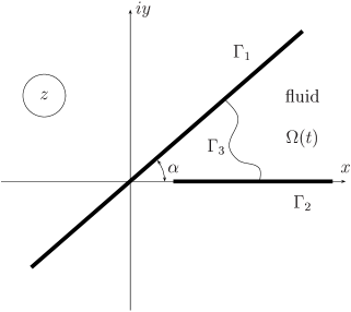
Figure 1. $\Omega(t)$ is the phase domain within an infinite corner and the homogeneous sink/source at $\infty$

In the zero-surface-tension model neglecting gravity, the unique acting force is pressure $p(z,t)\equiv p(x,y,t)$. The velocity field averaged across the gap is given by the Hele-Shaw law (Darcy’s law in the multidimensional case) as $\text{\bf V}=-\nabla p$. Incompressibility implies that $p(z,t)$ is simply

(1) $$\Delta p=0,\quad\mbox{in the flow region $\Omega(t)$.}$$

The dynamic condition

(2) $$p\Big{|}_{\Gamma_{3}}=0,$$

is imposed on the free boundary $\Gamma_{3}\equiv\Gamma_{3}(t)$. The kinematic condition implies that the normal velocity $v_{n}$ of the free boundary $\Gamma_{3}$ outwards from $\Omega(t)$ is given as

(3) $$\frac{\partial p}{\partial n}\Big{|}_{\Gamma_{3}}=-v_{n}.$$

On the walls $\Gamma_{1}\equiv\Gamma_{1}(t)$ and $\Gamma_{2}\equiv\Gamma_{2}(t)$ the boundary conditions are given as

(4) $$\frac{\partial p}{\partial n}\Big{|}_{\Gamma_{1}\cup\Gamma_{2}}=0,$$

(impermeability condition). We suppose that the motion is driven by a homogeneous source/sink at infinity. Since the angle between the walls at infinity is also $\alpha$, the pressure behaves about infinity as

$$p\sim\frac{-Q}{\alpha}\log|z|,\quad\mbox{as $|z|\to\infty$},$$

where $Q$ corresponds to the constant strength of the source ($Q<0$) or sink ($Q>0$). Finally, we assume that $\Gamma_{3}(0)$ is a given analytic curve.

We introduce the complex velocity (complex analytic potential) $W(z,t)=p(z,t)+i\psi(z,t)$, where $-\psi$ is the stream function. Then, $\nabla p=\overline{\partial W/\partial z}$ by the Cauchy-Riemann conditions. Let us consider an auxiliary parametric complex $\zeta$-plane, $\zeta=\xi+i\eta$. We set $D=\{\zeta:\,|\zeta|>1,\,0<\arg\zeta<\alpha\}$, $D_{3}=\{z:\,z=e^{i\theta},\,\theta\in(0,\alpha)\}$, $D_{1}=\{z:\,z=re^{i\alpha},\,r>1\}$, $D_{2}=\{z:\,z=r,\,r>1\}$, $\partial D=D_{1}\cup D_{2}\cup D_{3}$, and construct a conformal univalent time-dependent map $z=f(\zeta,t)$, $f:\,D\to\Omega(t)$, so that being continued onto $\partial D$, $f(\infty,t)\equiv\infty$, and the circular arc $D_{3}$ of $\partial D$ is mapped onto $\Gamma_{3}$ (see Figure 2).

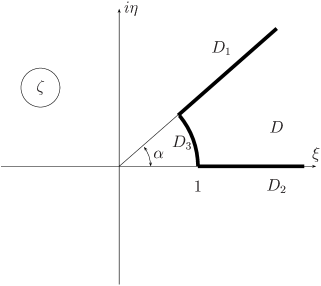
Figure 2. The parametric domain $D$

This map has the expansion

$$f(\zeta,t)=\zeta\sum\limits_{n=0}^{\infty}a_{n}(t)\zeta^{-\frac{\pi n}{\alpha}}$$

about infinity and $a_{0}(t)>0$. The function $f$ parameterizes the boundary of the domain $\Omega(t)$ by $\Gamma_{j}=\{z:\,z=f(\zeta,t),\,\zeta\in D_{j}\}$, $j=1,2,3$.

We will use the notations $\dot{f}=\partial f/\partial t$, $f^{\prime}=\partial f/\partial\zeta$. The normal unit vector in the outward direction is given by

$$\hat{n}=-\zeta\frac{f^{\prime}}{|f^{\prime}|}\,\,\,\mbox{on $\Gamma_{3}$, \ }\hat{n}=-i\,\,\,\mbox{on $\Gamma_{2}$, and \ }\hat{n}=ie^{i\alpha}\,\,\,\mbox{on $\Gamma_{1}$.}$$

Therefore, the normal velocity is obtained as

(5) $$v_{n}=\text{\bf V}\cdot\hat{n}=-\frac{\partial p}{\partial n}=\left\{\begin{array}[]{ll}-\text{\rm Re }\left(\displaystyle{\frac{\partial W}{\partial z}\frac{\zeta f^{\prime}}{|f^{\prime}|}}\right),&\mbox{for $\zeta\in D_{3}$}\\ 0,&\mbox{for $\zeta\in D_{1}$}\\ 0,&\mbox{for $\zeta\in D_{2}$}\end{array}\right.$$

The superposition $W\circ f$ is the solution to the mixed boundary problem (1), (2), (4) in $D$, therefore, it is the Robin function given by $W\circ f=-\frac{Q}{\alpha}\log\zeta$. On the other hand,

(6) $$v_{n}=\left\{\begin{array}[]{ll}\text{\rm Re }(\dot{f}{\overline{\zeta f^{\prime}}}/{|f^{\prime}|}),&\mbox{for $\zeta\in D_{3}$}\\ \text{\rm Im }(\dot{f}e^{-i\alpha}),&\mbox{for $\zeta\in D_{1}$}\\ -\text{\rm Im }(\dot{f}),&\mbox{for $\zeta\in D_{2}$}\end{array}\right.$$

The first lines of (5), (6) give us that

(7) $$\text{\rm Re }(\dot{f}\,\,{\overline{\zeta f^{\prime}}})=\frac{Q}{\alpha},\quad\mbox{for $\zeta\in D_{3}$}.$$

The resting lines of (5), (6) imply

(8) $$\text{\rm Im }(\dot{f}e^{-i\alpha})=0\quad\mbox{for $\zeta\in D_{1}$,$\quad$ }\text{\rm Im }(\dot{f})=0\quad\mbox{for $\zeta\in D_{2}$}.$$

3. Exact solutions in a wedge of arbitrary angle

We are looking for a solution in the form

$$f(\zeta,t)=\sqrt{\frac{2Qt}{\alpha}}\zeta+\zeta g(\zeta),$$

where $g(\zeta)$ is regular in $D$ with the expansion

$$g(\zeta)=\sum\limits_{n=0}^{\infty}\frac{a_{n}}{\zeta^{\frac{\pi n}{\alpha}}}$$

about infinity. The branch is chosen so that $g$, being continued symmetrically into the reflection of $D$ is real at real points. The equation (7) implies that on $D_{3}$ the function $g$ satisfies the equation

$$\text{\rm Re }(g(\zeta)+\zeta g^{\prime}(\zeta))=0,\quad\zeta\in D_{3}.$$

Taking into account the expansion of $g$ we are looking for a solution satisfying the equation

(9) $$g(\zeta)+\zeta g^{\prime}(\zeta)=\frac{\zeta^{\frac{\pi}{\alpha}}-1}{\zeta^{\frac{\pi}{\alpha}}+1},\quad\zeta\in D.$$

Changing the right-hand side of the above equation one would obtain other solutions. The general solution to (9) can be given in terms of the Gauss hypergeometric function $\text{\bf F}\equiv{{}_{2}\text{\bf F}}_{1}$ as

$$\zeta g(\zeta)=\zeta-2\zeta\text{\bf F}\left(\frac{\alpha}{\pi},1,1+\frac{\alpha}{\pi};-\zeta^{\frac{\pi}{\alpha}}\right)+C.$$

ht

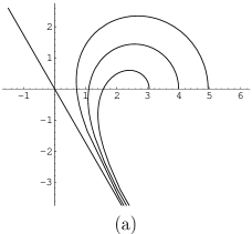
Figure 3. Interface evolution in the wedge of angle: (a) $\alpha=2\pi/3$; (b) $\alpha=\pi/3$

We note that $f^{\prime}$ vanishes for $\zeta^{\frac{\pi}{\alpha}}=(2/(1+\sqrt{2Qt/\alpha}))-1$, therefore, the function $f$ is locally univalent, the cusp problem is degenerating and appears only at the initial time $t=0$ and the solution exists during infinite time. The resulting function is homeomorphic on the boundary $\partial D$, hence it is univalent in $D$. This presents a case (apart from the trivial one) of the long existence of the solution in the problem with suction (ill-posed problem). To complete our solution we need to determine the constant $C$. First of all we choose the branch of the function ${}_{2}\text{\bf F}_{1}$ so that the points of the ray $\zeta>1$ have real images. This implies that $\text{\rm Im }C=0$. We continue verifying the asymptotic properties of the function $f(e^{i\theta},t)$ as $\theta\to\alpha-0$. The slope is

$$\lim\limits_{\theta\to\alpha-0}\arg[ie^{i\theta}f^{\prime}(e^{i\theta},t)]=\alpha+\frac{\pi}{2}+\lim\limits_{\theta\to\alpha-0}\arg\left(\sqrt{\frac{2Qt}{\alpha}}+\frac{e^{i\frac{\pi\theta}{\alpha}}-1}{e^{i\frac{\pi\theta}{\alpha}}+1}\right)=\alpha+\pi.$$

To calculate shift we choose $C$ such that

$$\lim\limits_{\theta\to\alpha-0}\text{\rm Im }[e^{-i\alpha}f^{\prime}(e^{i\theta},t)]=0.$$

Using the properties of hypergeometric functions we have

$$\lim\limits_{\gamma\to 0+0}\text{\rm Im }\text{\bf F}\left(\frac{\alpha}{\pi},1,1+\frac{\alpha}{\pi};e^{i\gamma}\right)=\frac{\alpha}{2}.$$

Therefore, $C=\alpha$. We present numerical simulation in Figure 3.

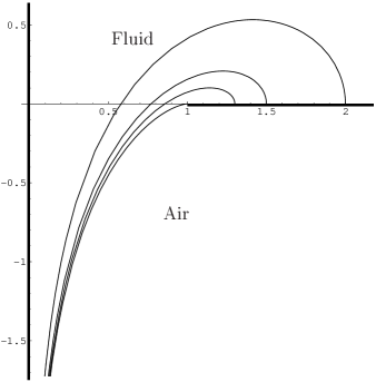
Figure 4. Kadanoff’s solution

The special case of angle $\alpha=\pi/2$ has been considered by Kadanoff [10]. The hypergeometric function is reduced to arctangent and we obtain

(10) $$f(\zeta,t)=(\sqrt{4Qt/\pi}+1)\zeta+i\log\frac{1+i\zeta}{1-i\zeta}+\frac{\pi}{2},\quad Q>0.$$

This function maps the domain $\{|\zeta|>1,\,\,0<\arg\,\zeta<\pi/2\}$ onto an infinite domain bounded by the imaginary axis $(\Gamma_{1})$, the ray $\Gamma_{2}=\{r:\,r\geq\sqrt{4Qt/\pi}+1\}$ of the real axis and an analytic curve $\Gamma_{3}$ which is the image of the circular arc, see Figure 4.

4. Perturbations of Kadanoff’s solution

Kadanoff’s solution (10) can be thought of as a logarithmic perturbation of a circular evolution with the trivial solution $f_{0}(\zeta,t)=\sqrt{4Qt/\pi}\zeta$. A simple way to generalize the solution (10) is to perturb another function. For example, one may choose

$$f_{0}(\zeta,t)=A\sqrt{t}\left(c\zeta+\frac{1}{c\zeta}\right),\quad c>1,\quad A=\sqrt{\frac{4Qc^{2}}{\pi(c^{4}-1)}}.$$

We find the solution $f(\zeta,t)$ in the form $f(\zeta,t)=f_{0}(\zeta,t)+h(\zeta)$ similarly to the preceding section. Then the equation (7) is satisfied when

$$\text{\rm Re }\frac{\zeta h^{\prime}(\zeta)}{\dot{f}_{0}(\zeta,t)}=0,\quad\mbox{or}\,\,\,\text{\rm Re }\frac{\zeta h^{\prime}(\zeta)}{c\zeta+1/c\zeta}=0,$$

where $h^{\prime}\sim(\zeta-i)^{-1}$ as $\zeta\to i$ in the unit circumference. We choose a consistent form of $h$ as

$$\frac{c\zeta^{2}h^{\prime}(\zeta)}{c^{2}\zeta^{2}+1}=\frac{\zeta^{2}-1}{\zeta^{2}+1}.$$

Integration yields

$$h(\zeta)=c\zeta+\frac{1}{c\zeta}-i\left(c-\frac{1}{c}\right)\log\frac{\zeta+i}{\zeta-i}+C,$$

where $C$ is a constant of integration. Satisfying the conditions on the walls we deduce that $C=0$, and finally, we get a logarithmic perturbation of the elliptic evolution as

$$f(\zeta,t)=(A\sqrt{t}+1)\left(c\zeta+\frac{1}{c\zeta}\right)-i\left(c-\frac{1}{c}\right)\log\frac{\zeta+i}{\zeta-i},$$

see the interface evolution in Figure 5.

Figure 5. Logarithmic perturbation of the elliptic evolution

The next goal is to obtain perturbations of the logarithmic term of Kadanoff’s solution that with the same asymptotic as $t\to\infty$, such that the interface has finite contact points at a finite moment. Let us consider the function

$$H(\zeta,t)=2d(t)\zeta-\log\frac{\zeta+a(t)}{\zeta-a(t)}.$$

The functions $a(t)$, $d(t)$ are to be chosen such that equation (7) is satisfied for the moving interface as well as the conditions of impermeability and univalence hold. The local univalence is followed from the first restriction $a(t)/d(t)<1$. Substituting $H$ into equation (7) and comparing the Fourier coefficients, we derive the following system of equations for the functions $a(t)$ and $d(t)$:

$$\left\{\begin{array}[]{l}(1+a^{4})d\dot{d}-a^{3}\dot{d}+da^{2}\dot{a}-a\dot{a}=\frac{Q}{2\pi}(1+a^{4}),\\ -2a^{2}d\dot{d}+a\dot{d}-\dot{a}d=-\frac{Q}{\pi}a^{2}\end{array}\right.$$

This system can be easily solved and the first integrals are

(11) $$d(t)=\frac{1+\sqrt{1+4a^{2}(t)(Qt/\pi-C_{1})}}{2a(t)},$$

(12) $$2\frac{d(t)}{a(t)}-\log\frac{1+a^{2}(t)}{1-a^{2}(t)}=C_{2},$$

where

$$C_{1}=-d^{2}(0)+\frac{d(0)}{a(0)},\quad C_{2}=2\frac{d(0)}{a(0)}-\log\frac{1+a^{2}(0)}{1-a^{2}(0)},$$

are the constants of integration. Let us assume the initial condition $a(0)\in(0,1)$. Making use of the system (11,12) we arrive at the explicit function $t(a)$ inverse to $a(t)$

(13) $$t(a)=\frac{\pi}{Q}\left(\frac{\left(a^{2}\log\frac{1+a^{2}}{1-a^{2}}+a^{2}C_{2}-1\right)^{2}-1}{4a^{2}}+C_{1}\right),$$

that exists, is continuous, and increases in the interval $a\in[a(0),1)$. Therefore, the function $a(t)$ increases from $a(0)$ to $1$ as $t\in[0,\infty)$. By (11) we conclude that $d(t)\sim O(\sqrt{t})$ as $t\to\infty$. The rotation of $H$ is exactly Kadanoff’s solution when $a=1$, and $d(t)$ is appropriately chosen as in (10). To make a numerical simulation one may use the Newton method of the solution of a non-linear system (Howison [7] presented the numerical approximation of an analogous solution in a narrow channel), see Figure 6.

Figure 6. Perturbation of Kadanoff’s solution for $a(0)=0.5$, $d(0)=1$

Choosing $a(0)$ rather close to 1, one may give an explicit analytic approximation by, e.g., introducing two functions

$$\hat{d}(t)=\frac{1+\sqrt{1+4(Qt/\pi-C_{1})}}{2},$$

$$\hat{a}(t)=\sqrt{\frac{\exp(2\hat{d}(t)-C_{2})-1}{\exp(2\hat{d}(t)-C_{2})+1}}.$$

The initial conditions $a(0)$ and $d(0)$ are to satisfy the inequalities $1-4C_{1}\geq 0$, $2\hat{d}(0)-C_{2}>0$. To proceed, we simplify putting $a(0)=d(0)$. Then these inequalities are satisfied for $d(0)\in(\sqrt{3/4},1)$. It is easily seen from (12) that $|1-a(t)|\sim e^{-\sqrt{t}}$. Then $|\hat{d}(t)-d(t)|\sim e^{-\sqrt{t}}$ too. Similarly, $\hat{d}(t)\sim\sqrt{t}$ and $|1-\hat{a}(t)|\sim e^{-\sqrt{t}}$. Both $\hat{a}(t)$ and $a(t)$ tend to 1 rapidly and the error $|\hat{a}(t)-a(t)|$ is of the same order for $t\sim\infty$.

Now we evaluate the error $|\hat{a}(t)-a(t)|$ for $0<t<\infty$, and claim that

(14) $$0<a(t)-\hat{a}(t)<8\big{(}a(0)-\hat{a}(0)\big{)}.$$

To prove this we estimate the distance $\rho(a)$ between the inverse function (13) and

$$\hat{t}(a)=\frac{\pi}{Q}\left(\frac{\left(\log\frac{1+a^{2}}{1-a^{2}}+C_{2}-1\right)^{2}-1}{4}+C_{1}\right),$$

as

$$\rho(a)=\hat{t}(a)-t(a)=(1-a^{2})\left(\log\frac{1+a^{2}}{1-a^{2}}+C_{2}\right)^{2}\quad\text{and}\quad\rho(a(0))=2(1-a(0)).$$

The derivative of $\rho$ is

$$\rho^{\prime}(a)=2a\left(\log\frac{1+a^{2}}{1-a^{2}}+C_{2}\right)\left(\frac{4}{1+a^{2}}-\log\frac{1+a^{2}}{1-a^{2}}-C_{2}\right).$$

Since the function $\log\frac{1+a^{2}}{1-a^{2}}$ increases, the function $\rho(a)$ may have a critical point $a_{c}$, $a_{c}\in[a(0),1)$, which is the maximal solution to the equation $\frac{4}{1+a_{c}^{2}}=\log\frac{1+a_{c}^{2}}{1-a_{c}^{2}}-C_{2}$ in the interval $[a(0),1)$. The latter equation implies

$$\rho(a_{c})=(1-a_{c}^{2})\left(\log\frac{1+a_{c}^{2}}{1-a_{c}^{2}}+C_{2}\right)^{2}=\frac{16(1-a_{c}^{2})}{\big{(}1+a_{c}^{2}\big{)}^{2}}\leq 16(1-a(0)^{2})=8\rho(a(0)),$$

that proves (14).

Moreover, $a(0)-\hat{a}(0)$ is decreasing and non-negative as a function of the initial condition $a(0)$, that vanishes as $a(0)\to 1$. Therefore, given a small positive number $\varepsilon$, we may choose $a(0)=d(0)$ close to 1 such that $\hat{a}(t)$ approximates $a(t)$ with the precision $\varepsilon$ during the whole time $0<t<\infty$. Desired quantity $a(0)$ satisfies the equation

$$a(0)-\sqrt{\frac{\exp{\Big{(}\sqrt{4a(0)^{2}-7}+\log\frac{1+a(0)^{2}}{1-a(0)^{2}}-1\Big{)}}-1}{\exp{\Big{(}\sqrt{4a(0)^{2}-7}+\log\frac{1+a(0)^{2}}{1-a(0)^{2}}-1\Big{)}}+1}}=\frac{\varepsilon}{8}.$$

A similar conclusion may be made for the function $d(t)$ and its approximation $\hat{d}(t)$ (note that $d(t)<\hat{d}(t)<1$). Moreover, the mapping

$$\hat{H}(\zeta,t)=2\hat{d}(t)\zeta-\log\frac{\zeta+\hat{a}(t)}{\zeta-\hat{a}(t)}$$

converges to Kadanoff’s solution as $t\to\infty$.

Figure 7. Error $|\hat{a}(t)-a(t)|$, for $a(0)=0.9$, $d(0)=0.9$

References

- [1] A. Arnéodo, Y. Couder, G. Grasseau, V. Hakim, M. Rabaud, Uncovering the analytical Saffman-Taylor finger in unstable viscows fingering and diffusion-limited aggregation, Phys. Rev. Lett. 63 (1989), no. 9. 984–987.
- [2] M. Ben Amar, Exact self-similar shapes in viscows fingering, Phys. Review A 43 (1991), no. 10, 5724–5727.
- [3] M. Ben Amar, Viscous fingering in a wedge, Phys. Review A 44 (1991), no. 6, 3673–3685.
- [4] L. J. Cummings, Flow around a wedge of arbitrary angle in a Hele-Shaw cell, European J. Appl. Math. 10 (1999), 547–560.
- [5] L. A. Galin, Unsteady filtration with a free surface, Dokl. Akad. Nauk USSR 47 (1945), 246–249. (in Russian)
- [6] Yu. E. Hohlov, S. D. Howison, On the classification of solutions to the zero-surface-tension model for Hele-Shaw free boundary flows, Quarterly of Appl. Math. 51 (1993), no. 4, 777–789.
- [7] S. D. Howison, Fingering in Hele-Shaw cells, J. Fluid Mech. 167 (1986), 439-453.
- [8] S. D. Howison, Complex variable methods in Hele-Shaw moving boundary problems, European J. Appl. Math. 3 (1992), no. 3, 209–224.
- [9] S. D. Howison, J. King, Explicit solutions to six free-boundary problems in fluid flow and diffusion, IMA J. Appl. Math. 42 (1989), 155–175.
- [10] L. P. Kadanoff, Exact soutions for the Saffman-Taylor problem with surface tension, Phys. Review Letters 65 (1990), no. 24, 2986–2988.
- [11] I. Markina, A. Vasil’ev, Explicit solutions for the Hele-Shaw corner flows, European J. Appl. Math. 15 (2004), no. 6, 781–789.
- [12] P. Ya. Polubarinova-Kochina, On a problem of the motion of the contour of a petroleum shell, Dokl. Akad. Nauk USSR 47 (1945), no. 4, 254–257. (in Russian)
- [13] P. G. Saffman, G. I. Taylor, The penetration of a fluid into a porous medium or Hele-Shaw cell containing a more viscous liquid, Proc. Royal Soc. London, Ser. A 245 (1958), no. 281, 312–329.
- [14] A. Vasil’ev, Univalent functions in two-dimensional free boundary problems, Acta Applic. Math. 79 (2003), no. 3, 249–280.