Neighborhood properties of complex networks

Abstract

A concept of neighborhood in complex networks is addressed based on the criterion of the minimal number os steps to reach other vertices. This amounts to, starting from a given network $R_{1}$, generating a family of networks $R_{\ell},\ell=2,3,...$ such that, the vertices that are $\ell$ steps apart in the original $R_{1}$, are only 1 step apart in $R_{\ell}$. The higher order networks are generated using Boolean operations among the adjacency matrices $M_{\ell}$ that represent $R_{\ell}$. The families originated by the well known linear and the Erdös-Renyi networks are found to be invariant, in the sense that the spectra of $M_{\ell}$ are the same, up to finite size effects. A further family originated from small world network is identified.

Several properties of complex networks have been addressed recently, much inspired by the identification of their relevance in the description of the relations among the individual constituents of many systems, which have their origin from natural to social sciences, telephone and internet to energy supply, etc. [1, 2, 3, 4]. The huge development in this research area came along with the proposition of many parameters that might be relevant to the characterization of properties of networks. The sofar most established and quantifiers are the distribution of links $n(k)$, clustering coefficient $C$, mean minimal distance among the nodes $<d>$, diameter $D$, the assortativity degree [5, 6]. The evaluation of these and other indices for actual networks help characterizing them, putting into some network classes with well defined properties, such as the small-world [7], the scale-free [8], the Erdös-Renyi [9] or random networks, etc.

As the number of nodes directly connected to node $i$ is $k_{i}$, $n(k)$ characterizes the immediate neighborhood of the network nodes. In this work we explore further neighborhood properties of networks, which are related to the distribution of the number of second, third, …, neighbors. For the sake of simplicity, we assume that the networks we consider herein are connected, i.e., each node can be reached from any other one. Two nodes are $\ell-th$ neighbors, or neighbors of order $O(\ell)$, when the minimal path connecting them has $\ell$ steps. Then, for a given network $R$, the explicit evaluation of the distributions of neighbors $O(\ell)$ along the network, $\ell=1,2,3,...$ promptly indicates the structure of minimal paths connecting the nodes. This classifies uniquely the neighborhood of a vertex, in the sense that if two vertices are $O(\ell)$ neighbors, they are not $O(j)$ neighbors for $\ell\neq j$. Also, we consider that any vertex is $O(0)$ neighbor of itself.

It is expected that the neighborhood properties change with $\ell$. However, if a meaningful criterion $G$ can be devised, according to which the $\ell$-neighborhoods of $R$ remain invariant, it may be important to assign $R$ a $G$ neighborhood invariant (NI) property. It characterizes an invariance of $R$ with respect to length scale, provided length is measured by number of steps along the network. Also, it is distinct both from the scale free distribution of vertex connections, as well as from geometrical scale invariance included in the construction of the network as, for instance, in the class of Apollonian networks (AN).

In our investigation we identified, for each $\ell$, all $O(\ell)$ neighbors of $R$ and constructed a family of networks ${\mathbf{R}}$. Each $R_{\ell}\in\mathbf{R}$ is defined by the same set of nodes, while links are inserted between all pairs of vertices that are $O(\ell)$ neighbors in $R\equiv R_{1}$. Thus, the family $\mathbf{R}$ characterizes the neighborhood structure of $R$. The $R_{\ell}$’s were actually set up by a corresponding family ${\mathbf{M}}$ of adjacency matrices (AM) ${M_{\ell}}$ [5], achieved by the systematic use of Boolean ($B$) operations [10] among matrices.

To define a neighborhood invariance criterion, it is necessary to identify a relevant network property that may be present in all elements of ${\mathbf{R}}$, e.g., the corresponding values for $n_{\ell}(k)$ and $C_{\ell}$ [11]. However, these are global indices that do not provide a sufficiently precise identification of a network. A much more precise characterization is based on the eigenvalue spectra of the family ${M_{\ell}}$[12, 13], even if it is well known that there may exist topologically distinct networks which share the same spectrum (co-spectral), and that only the complete set of eigenvalues and eigenvectors univocally characterizes a network. A spectrum based invariance criterion condenses (in the sense of reducing from $N^{2}$ elements of $M$ to $N$ numbers) a lot of information about the network, and has been used herein. This can be further justified by the fact that, if two AM’s in ${M_{\ell}}$ have the same spectrum, they differ only by a basis transformation.

Before proceeding with details of the guidelines of our actual work, we recall that the first matrix $M_{1}$, which describes the original network $R_{1}$, has only 0’s or 1’s as entries for all of its elements. If $M_{1}$ is applied to a unitary vector $v_{\ell}$, with all but one entry $\ell$ set to 0, the resulting vector expresses which vertices are linked to the the vertex $\ell$. If we take the usual matrix product of $M_{1}$ by itself, the non-zero elements $(M_{1}^{2})_{rs}$ of the resulting matrix $M_{1}^{2}$ indicates how many possible two-step walks along the network, with endpoints $r$ and $s$ exist. Contrary to what happens with $M_{1}$, $M_{1}^{2}$ has many elements $(M_{1}^{2})_{rs}>1$, indicating multiplicity of paths starting at $r$ and ending at $s$. In particular, all elements $(M_{1}^{2})_{rr}$ of the diagonal can have this property, since they count all two-step walks that start at $r$, visit any of the vertices $s$ to which $r$ is linked $(M_{1})_{rs}=1$, and turn back to $r$. The same interpretation is valid for all usual powers of $M_{1}$.

As the elements of $M_{1}$ are all 0’s or 1’s, we can regard $(M_{1})_{rs}$ as $B$ variables, and use the $B$ sum, subtraction and product operations [10], respectively $\oplus,\ominus,\otimes$,

$$\begin{array}[]{llll}0\oplus 0=0&1\oplus 0=1&0\oplus 1=1&1\oplus 1=1\\ 0\ominus 0=0&1\ominus 0=1&0\ominus 1=0&1\ominus 1=0\\ 0\otimes 0=0&1\otimes 0=0&0\otimes 1=0&1\otimes 1=1\end{array}$$ (1)

to define $B$ operations between matrices of $B$ elements. The $B$ matrix operations are defined by using the usual matrix element operation rules, replacing the usual sum, subtraction and product involving matrix elements by the corresponding $B$ operations. To avoid multiplicity of notation, we will use hereafter the same symbols $\oplus,\ominus$ and $\otimes$ to indicate matrix $B$ operations.

If we consider $\overline{M_{2}}=M_{1}\otimes M_{1}$ and compare it to $M_{1}^{2}$, we see that the position of all their zero elements coincides, while if we collapse to 1 all non-zero elements of $M_{1}^{2}$ we obtain $\overline{M_{2}}$. In fact, $\overline{M_{2}}$ indicates the possibility of two-step walks, while it deletes the information on the multiplicity of walks. As the neighborhood concept does not take path multiplicity into account, the $B$ operations are well suited to define the matrices $M_{i}$.

For instance, $M_{2}$ can be expressed by

$$M_{2}=(M_{1}\oplus\overline{M_{2}})-(I\oplus M_{1})=(I\oplus M_{1})\otimes M_{1}-(I\oplus M_{1}),$$ (2)

where $I$ indicates the identity matrix. To see this note that all forward-backward walks, included together with pairs of distinct sites linked by two-step walks in $\overline{M_{2}}$, can not be present in $M_{2}$, as any vertex has been defined to be $O(0)$ neighbor of itself. Thus we must subtract $I$ from $\overline{M_{2}}$. Also, it is necessary to $B$ sum $M_{1}$ to $\overline{M_{2}}$, and subsequently subtract $M_{1}$, as $\overline{M_{2}}$ may describe two-step walks between two sites that were already related in the original network $R_{1}$. Noting that $M_{0}\equiv I$, Eq.(2) can be generalized for arbitrary value of $\ell$ by:

$$M_{\ell}=(\bigoplus_{j=0}^{\ell-1}M_{j})\otimes M_{1}-(\bigoplus_{j=0}^{\ell-1}M_{j})=M_{\ell-1}\otimes M_{1}\ominus(\bigoplus_{j=0}^{\ell-1}M_{j}).$$ (3)

Once a precise procedures to set up all $M_{\ell}$’s is available, let us briefly comment on several possibilities opened by the knowledge of ${\mathbf{M}}$ for the purpose of evaluation of network indices. 1) If we have a finite network with $\mathbf{N}$ vertices, then there is a large enough $\ell_{max}$ such that $M_{\ell}\equiv 0,\forall\ell>\ell_{max}$. Thus, the value for $D$ is found when the first $M_{\ell}\equiv 0$ is found. Also, when $\ell$ approaches $D$, the $M_{\ell}$’s become sparser and, as a consequence, the number of zero eigenvalues increases largely. 2) As for each $r,s$ pair, $(m_{\ell})_{rs}=1$ for only one ${M_{\ell}}\in\mathbf{M}$, one can collapse in a single matrix

$$\widehat{M}=\sum_{j=0}^{\ell_{max}}jM_{j}$$ (4)

all information on the neighborhood of any pairs of vertices. Particularly, all pairs $r,s$ of the $O(\ell)$ neighbors satisfy $\widehat{M}_{rs}=\ell$. 3) To obtain the average minimal path for each node $r$, it is sufficient to sum all elements of the $r-th$ row (or column) of $\widehat{M}$ and divide by $\mathbf{N}-1$. The average minimal path for the network follows immediately. 4) The evaluation of all $C_{\ell}$ by means of line to line multiplication of matrix elements, can be easily computed once the family ${\mathbf{M}}$ has been obtained. 5) The matrix $\widehat{M}$ can be easily used to visualize the structure of network with the help of a color or grey code plots.

The numerical evaluation of the eigenvalue spectra ${\lambda_{\ell}^{r},r\in[1,\mathbf{N}]}$ for the family ${M_{\ell}}$ has been carried out for several networks. For each one of them, we are particularly interested to understand how the form of the spectral density $\rho_{\ell}(\lambda)$ as function of $\lambda$ evolves with $\ell$. We first illustrate the procedure by showing how the spectra of the standard AN depends on $\ell$. Several properties of AN’s have been discussed recently [14, 15]: they are constructed according to a precise geometrical iteration rule that grant them topological self-similarity and a scale free distribution of nodes degrees. The $M_{1}$ spectra of the AN for $g$ successive generations converge very quickly to a well defined form. However, for the finite size networks up to $g=8$, with 3283 vertices, we can not identify any sort of invariance in the eigenvalues density distribution $\rho_{\ell}(\lambda)$. This is better visualized with the help of the integrated spectra [16]

$$\Pi_{\ell}(\lambda)=\frac{1}{N}\int_{-\infty}^{\lambda}\rho_{\ell}(\lambda^{\prime})d\lambda^{\prime},$$ (5)

for successive generations, as shown in the Figure 1. $\Pi_{1}$ and $\Pi_{2}$ converge very quickly to distinct $g$ independent forms. Thus, scale free distribution of node degrees and self similarity do not necessarily lead to NI.

Figure 1: Plots of $\Pi\times\lambda$ for $M_{1}$ (solid) and $M_{2}$ (dashed) of the AN, when $g=7$ and 8

Exact NI invariance is observed for the linear chain network with periodic boundary conditions, where each vertex interacts only with its two next neighbors. The corresponding AM $M_{1}$ has a well known pattern, where all 1 elements are placed along the nearest upper and lower diagonals to the matrix main diagonal. This matrix has been used to describe a very large number of models in 1 dimension, like the system of phonons, tight-binding electrons [17, 18], etc. Also, it has been used as the starting point to construct small world networks, by changing some of the original nearest neighbors links according to a given rewiring probability $p_{w}$. For $M_{1}$, $\rho$ is expressed analytically by the relation [17, 18, 19]

$$\rho(\lambda)\sim\frac{1}{(4-\lambda^{2})^{1/2}}.$$ (6)

The other matrices of the family ${M_{\ell}}$ keep essentially the same shape, with two sequences of 1’s along near-diagonals. Each one of them moves one step away from the main diagonal upon increasing the value of $\ell$ by 1, but this does not change the spectrum. Indeed, this operation can be regarded, e.g. in the analysis of tight-binding systems, as a decimation procedure of half of the sites along with a renormalization of the hopping integral [19]. The resulting system has exactly the same shape as the original and, consequently, the same spectral density. The diameter of the network depends linearly on $\mathbf{N}$, as diagonals move away one step when $\ell$ is increased by 1.

Figure 2: Spectral density $\rho_{\ell}$ for the Erdös-Rényi network single realizations. (a) $\mathbf{N}=1000,p=0.05,\ell=1,2,3,4,5$. (b) Scaled $\rho_{2}$ for conditions $p=c/N^{z}$, when $c=68,z=0.9,N=500,1000,3000,3500$

The Erdös-Renyi networks [9] constitute another class where one could expect to find NI. Indeed, if connections are randomly distributed for $R_{1}$, so should they also be for all members of R. For very low values of $p$ (the connection probability between any two nodes), $R_{1}$ is split into several disjoint clusters, and this situation is preserved for all other $R_{\ell}$’s. In such cases, the $M_{1}$ spectral density does not obey a simple analytical expression, being constituted by some individual peaks superimposed on a shallow background. The $M_{\ell}$ ($\ell\geq 2$) spectra also share the same qualitative structure. Quantitatively, it is observed an increase of the $\lambda=0$ dominant peak and a decrease of the other peaks. This is related to the clustered structure of the network and to the fact that several clusters are reaching their own diameter.

When $p=c/N^{z}$, with $z<1$, and for such large enough $c$, almost all nodes are connected in a single cluster, and $\rho$ obeys the well known semicircle law [20, 21]

$$\rho(\lambda)\sim(4-\lambda^{2})^{1/2}.$$ (7)

In this regime, networks usually have a very small diameter, and invariance can only be noted for a few values of $\ell$. For the average node number $\langle k\rangle\simeq 0.5$, we have found that the $\rho_{2}$ also obeys (7), as shown in the Fig. 2b. However, for smaller values of $\langle k\rangle$, a clear skewness in the distribution is observed for $\rho_{2}$, despite the semicircle form of $\rho_{1}$. We conclude that Erdös-Renyi networks are NI for a restricted subset of $p$ and $c$.

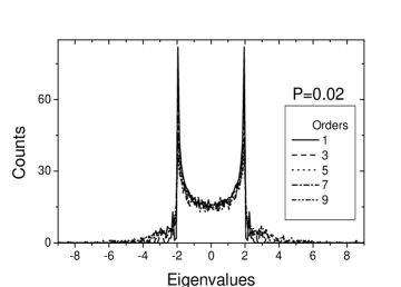
Figure 3: Plots of the spectra $\rho\times\lambda$ of the matrices $M_{\ell},\ell=1,3,5,7,9$, for a Watts-Strogatz small world network starting from a nearest neighbor linear chain and $p_{w}=0.02$.

We have also investigated small world networks obtained along the Watts-Strogatz rewiring procedure[7], starting both from the above discussed next-neighbor (nn) and the nearest-next-neighbor (nnn) linear chains. In Figure 3, we show a sequence of $M_{\ell}$ spectra for very small value of $p_{w}$, starting from a nn chain. We see that the $\rho(\lambda)$ is split into two parts: the first one, essentially described by Eq.(6), corresponds to the contribution of unperturbed segments of the linear chain. We see that, as it happens to the whole spectra when $p_{w}=0$, this part remains almost invariant, at least for a large number of $M_{\ell}$. The other part of the spectra, located outside of this first region, has no well defined shape. It entails a considerably lower number of eigenvalues, which increases with $\ell$. This indicates that, at each increase of $\ell$, a small number of eigenvalues migrates from the unperturbed part into it, as the number of vertices that are affected by the rewiring operation increases with $i$. This successive migration ends up by affecting the whole form of the spectrum for large enough $\ell$. Of course this behavior depends on the value of $p_{w}$. If we increase it, there is a smooth transition on the shape of the $M_{1}$ spectrum, until it reaches a pattern with many structures and bands, similar to that of the AN.

Figure 4: Almost invariant spectra $\rho\times\lambda$ of the matrices $M_{\ell},\ell=7-10$, for a Watts-Strogatz- small network starting from a next-nearest neighbor linear chain and $p_{w}=0.2$.

For $p_{w}$ in the range $p_{w}\sim 0.15-0.22$, we have observed that, as $\ell$ increases, the spectral density $\rho_{\ell}$ evolves towards a very peculiar form, which remains almost invariant for several values of $\ell$, as shown in the Figure 4. This spectrum has its own features, distinct from those discussed before for the fully ordered and disordered networks. For the specific case $p_{w}=0.21$ and $\mathbf{N}=1000$, we have a large diameter $D=15$, and the shown form of the spectra remains invariant for $\ell\in[7,10]$. For smaller values of $\ell$, the shape changes steadily from a structured shapes similar to those in Figure 3 into the invariant form. For larger values of $\ell$, finite size effects lead to quite sparse $M_{\ell}$, with a large number of zero eigenvalues: $\rho_{\ell}$ evolves to a $\delta$ like distribution centered at $\lambda=0$.

This effect can be graphically illustrated with the help of the matrix $\widehat{M}$. In Figure 5 we draw the position of the $O(\ell)$ neighbors for three distinct ranges of $\ell$. The particular shape in Figure 4 is associated with roughly dense matrices when $\ell\in[7,10]$. For smaller and larger values of $\ell$, matrices have rather distinct structure.

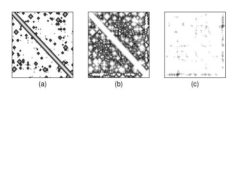
Figure 5: For the same Watts-Strogatz small network of Figure 4, graphical illustration of distribution of $O(\ell)$ neighborhoods: $\ell\in[1,6],[7,10],[11,15]$ for (a), (b) and (c) respectively.

For other values of $\mathbf{N}$, we have observed the same evolution. For instance, when $\mathbf{N}=1500$ and $2000$, the shape lasts almost invariant for more generations, respectively $\ell\in[8,12]$ and $[11,16]$, indicating that this behavior can be more robust as $\mathbf{N}$ increases. For $p_{w}$ larger than the range given above, this persistence in the form is not observed. For smaller values of $p_{w}$ the spectra changes very slowly as shown in Figure 3. In such cases, finite size effects set in prior than any tendency of evolution towards the form shown in Figure 4.

To conclude, in this work we have discussed the concept of higher order neighborhood and neighborhood invariance of networks. These have been obtained by a systematic use of Boolean matrix operations and the definition of a AM family. We explored well-know networks, showing that this property is not equivalent to other concepts of scale and geometrical invariance. Further, we looked for evidence of NI based on the invariance of the spectral density, identifying this property in the linear chain, Erdös-Renyi network, and finally, in a non-trivial class that evolves from Watts small world network.

Acknowledgement: This work was partially supported by CNPq and FAPESB.

References

- [1] D. J. Watts Small Worlds: The Dynamics of Networks between Order and Randomness, (Princeton University Press, 1999).
- [2] A. L. Barabasi, Linked: The New Science of Networks, (Perseus Books Group, Cambridge MA, 2002).
- [3] S. N. Dorogovtsev and J. F. F. Mendes, Evolution of Networks: From Biological Nets to the Internet and WWW, (Oxford Univ. Press, 2003).
- [4] R. Pastor-Satorras and A. Vespignani, Evolution and Structure of the Internet: A Statistical Physics Approach, (Cambridge University Press, 2004).
- [5] R. Albert, and A.L. Barabasi, Rev. Mod. Phys 74, 47 (2002).
- [6] M.E.J. Newman, Phys. Rev. Lett. 89, 208701 (2002).
- [7] D. J. Watts and S.H. Strogatz, Nature 393, 440 (1998).
- [8] A.L. Barabasi, and R. Albert, Science 286, 509 (1999).
- [9] P. Erdös, and A. Rényi, Publ. Math. (Debrecen), 6, 290 (1959).
- [10] J.E. Whitesitt, Boolean Algebra and its Applications, (Dover, New York, 1995).
- [11] A.Fronczak, J.A. Holyst, M. Jedynak, and J.Sienkiewicz, Physica A 316, 688 (2002).
- [12] B. Bolobás, Random Graphs, (Academic Press, London, 1985).
- [13] D.M. Cvetkovic, M. Dods, H. Sachs, Spectra of Graphs, (Academic Press, New York, 1979).
- [14] J.S. Andrade Jr., H.J. Herrmann, R.F.S. Andrade, L.R. Silva, Phys. Rev. Lett. 94, 018702 (2005).
- [15] J.P.K. Doye, and C.P. Massen, Phys. Rev. E 71, 016128 (2005).
- [16] R.F.S. Andrade, and J.G.V. Miranda, Physica A, (2005).
- [17] N.W. Ashcroft, and N.D. Mermin, Solid State Physics,(Holt-Saunders, New York, 1976).
- [18] E. N. Economou, Green’s Function in Quantum Physics, (Springer, Berlin, 1979).
- [19] C.E.T. Gonçalves da Silva, and B. Koiller, Solid State Commun. 40, 215 (1981).
- [20] E.P. Wigner, Ann. Math. 62, 548 (1955).
- [21] A. Crisanti, G. Paladin, and A. Vulpiani, Products of Random Matrices in Statistical Physics, Springer, Berlin, 1993.