Bound and Trapped Classical States of an Electric Dipole in Magnetic Field

Abstract

In the present work, we study the classical behavior of an electric dipole in presence of an external uniform magnetic field. We derive equations and constants of motion from the Lagrangian formulation. We obtain an infinitely periodic effective potential that describes a rotational motion. The problem is not directly separable in relative and center of mass variables; even though, we are able to write the energy of the system as a function of an only term, the relative variable. We define another constant of motion, which couples the relative with the center of mass variables. We describe conditions for bound states of the dipole. In addition, we discuss the problem in the approximation of small oscillations. Finally, we explore the existence of a possible family of trapped states in a region of the space where there are no classical turning points.

I Introduction

Nowadays, fundamental elements in scale of molecular machineryscience306 ; science281 ; nat406_605 ; nat406_608 ; nat401_150 ; nat401_152 take the attention from several specialists, due to the development of nanotechnology. An alternating electric field has already used to explore electronic structures, however this process can be useful to exchange the orientation of molecules; therefore, it is possible to obtain some controlled molecular motion by oscillating electric fieldsnat406_608 . Devices on the molecular level are obtained from the conversion of energy into controlled motion; regardless of this, it is difficult to repeat this process in a mechanical molecular motor. This process is common in biological systemsnat406_605 . By moment, it is expected to find physical principles of a motor in molecular scale through the dynamics of rotors in two dimensions. Such rotors are modeled as electric dipoles in electric or magnetic fields.

It is well known, we know that the simplest many-body system is the two-body system and we expect to separate the two-body problem in two problems of a single body. The problem of two equal charges in an external magnetic field fulfills to this requirement completely. In a suitable formulation, two independent variables are considered to describe the motion of the center of mass and the relative motion, respectively. The classicalajp65 and quantumpla269 physics of the problem are clearly described in details . On other hand, the problem of two particles with opposite charges into a magnetic field does not allow to make the separation of variables in independent equations, as it is possible to do it in the case presented above. Nevertheless, two constants of motion are obtained from a suitable Lagrangian formulation. It is possible to write an equation for the energy in terms of the relative variable and other constant of motion connecting the relative variable with the center of the mass coordinate. Classicalajp65 and quantumjpa2 results were previously reported.

In addition, other related cases are discussed in precedent works

• the dynamics of charges in oscillating electric and magnetic fields in Ref.BJP29 ; pra59 ,

• the dynamics of a dipole in a magnetic field on $Y$ direction, the motion of its center of mass is restricted to the $Z$ direction, and its rotation to the $XY$ plane, is discussed in Ref.Pursey .

The main goal in this work is to describe the classical behavior of an electric dipole in an external magnetic field. With this purpose, we introduce a model for an electric dipole as two particles of arbitrary masses, where separation between them is constant, and its charges are equal and opposite. That case is a two-body problem and its exact analysis requires a difficult treatment and the further useful understanding, which is obtained by approximations.

The paper is organized as follows. Firstly, we present a general formulation for an electric dipole in magnetic field. We define the Lagrangian function and we derive constants and equations of motion. Secondly, we present the solution for a particular problem; this is, the planar motion of an electric dipole in a perpendicular magnetic field. We discuss bound and trapped states. Finally, we summarize the formulation and main results.

II Lagrangian Formulation: Symmetric Gauge

In the present model, internal coupling holds the two charges of the dipole together and the Coulomb interaction between the charges comes to be constant. Then, we consider a rigid dipole, two fixed charges by a massless rod, in the presence of a uniform magnetic field. One of particles carries charge $+e$, while the other $-e$. The magnetic field is derived from a vector potential $\vec{A}$, as follows $\vec{B}=\nabla\times\vec{A}$. We relate to the particle $1(2)$ the position ${\vec{r}}_{1}({\vec{r}}_{2})$, the velocity $\dot{\vec{r}}_{1}(\dot{\vec{r}}_{2})$ and the mass $m_{1}(m_{2})$. The Lagrangian formulation leads to the following expression:

$$L(\vec{r}_{1},\vec{r}_{2};\dot{\vec{r}}_{1},\dot{\vec{r}}_{2})=\frac{1}{2}m_{1}{\dot{\vec{r}}_{1}}^{2}+\frac{1}{2}m_{2}{\dot{\vec{r}}_{2}}^{2}-\frac{e}{c}\vec{A}(\vec{r}_{1})\cdot\dot{\vec{r}}_{1}+\frac{e}{c}\vec{A}(\vec{r}_{2})\cdot\dot{\vec{r}}_{2}+\frac{e^{2}}{\kappa|\vec{r}_{2}-\vec{r}_{1}|}$$ (1)

where $\kappa$ is the dielectric constant of the medium in which the motion of the dipole occurs. We define the vector potential $\vec{A}$ through the symmetric gauge as follows

$$\vec{A}(\vec{r}_{i})=\frac{1}{2}\vec{B}\times\vec{r}_{i},\mbox{ for $i$=1, 2},$$ (2)

where $\vec{B}$ is the uniform magnetic field. Now, we take into account the following change of variables

$$\vec{r}=\vec{r}_{2}-\vec{r}_{1},$$ (3)

$$\vec{R}=\frac{m_{1}\vec{r}_{1}+m_{2}\vec{r}_{2}}{m_{1}+m_{2}},$$ (4)

where $\vec{r}$ is the relative position and $\vec{R}$ is the position of the center of mass. Now, if we replace Eq.(2)-Eq.(4)into Eq.(1), we obtain the following function

$$L(\vec{R},\vec{r};\dot{\vec{R}},\dot{\vec{r}}) = \frac{1}{2}M{\dot{\vec{R}}}^{2}+\frac{1}{2}\mu{\dot{\vec{r}}}^{2}+\frac{e^{2}}{\kappa|\vec{r}|}$$ (5)

$$+ \frac{e}{c}\left[\frac{1}{2}\vec{B}\times\vec{R}\cdot\dot{\vec{r}}+\frac{1}{2}\vec{B}\times\vec{r}\cdot\dot{\vec{R}}+\frac{(m_{1}-m_{2})}{M}\frac{1}{2}\vec{B}\times\vec{r}\cdot\dot{\vec{r}}\right]$$

where $M=m_{1}+m_{2}$ is the mass of the center of mass and $\mu=m_{1}m_{2}/M$ is the reduced mass. From now on, we consider $m_{1}=m_{2}$. In contrast to the case of two identical particlesajp65 ; pla269 , the present Lagrangian function is similar to particles with opposite charges because it is a nonseparable problem; the motion of the center of mass is coupled to the relative variableajp65 . The conjugate momentum for the center of mass is given by

$$\vec{P}_{\vec{R}}=\frac{\partial L(\vec{R},\vec{r};\dot{\vec{R}},\dot{\vec{r}})}{\partial\dot{\vec{R}}}=M\dot{\vec{R}}+\frac{e}{2c}\vec{B}\times\vec{r},$$ (6)

which depends on center of mass and relative motions. From deriving the equations of motion we have

$$\dot{\vec{P}}_{\vec{R}}=\frac{\partial L(\vec{R},\vec{r};\dot{\vec{R}},\dot{\vec{r}})}{\partial\vec{R}}=-\frac{e}{2c}\vec{B}\times\dot{\vec{r}}$$ (7)

If we integrate the Eq.(7), and it compares with the Eq.(6), we obtain the first constant of motion

$$M\dot{\vec{R}}+\frac{e}{c}\vec{B}\times\vec{r}\equiv\vec{C},$$ (8)

and the first equation of motion is given by

$$M\ddot{\vec{R}}=-\frac{e}{c}\vec{B}\times\dot{\vec{r}}.$$ (9)

We obtain for the relative vector conjugate momentum

$$\vec{p}_{\vec{r}}=\frac{\partial L(\vec{R},\vec{r};\dot{\vec{R}},\dot{\vec{r}})}{\partial\dot{\vec{r}}}=\mu\dot{\vec{r}}+\frac{e}{2c}\vec{B}\times\vec{R},$$ (10)

thus, the force is given by

$$\dot{\vec{p}}_{\vec{r}}=\frac{\partial L(\vec{R},\vec{r};\dot{\vec{R}},\vec{r})}{\partial{\vec{r}}}=-\frac{e}{c}{\vec{B}}\times\dot{\vec{R}}-\frac{e^{2}}{\kappa{|\vec{r}|}^{2}}\hat{e_{r}}.$$ (11)

If we derive the Eq.(10) in time, and we compare with Eq.(11), we can obtain the second equation of motion

$$\mu\ddot{\vec{r}}=-\frac{e}{c}\vec{B}\times\dot{\vec{R}}-\frac{e^{2}}{\kappa{|\vec{r}|}^{2}}\hat{e_{r}}.$$ (12)

The second constant of motion is $E$, the energy of the system. The general way to calculate the energy from a knowledge $L$ is

$$E=E(\vec{R},\vec{r};\dot{\vec{R}},\vec{r})=\vec{P}_{\vec{R}}\cdot\dot{\vec{R}}+\vec{p}_{\vec{r}}\cdot\dot{\vec{r}}-L(\vec{R},\vec{r};\dot{\vec{R}},\vec{r}),$$ (13)

and if we take Eq.(5) and we replace it into Eq.(13) we can explicitly obtain

$$E=\frac{1}{2}M{\dot{\vec{R}}}^{2}+\frac{1}{2}\mu{\dot{\vec{r}}}^{2}-\frac{e^{2}}{\kappa|\vec{r}|},$$ (14)

Putting Eq.(8) in Eq.(14), we obtain an expression for the energy in terms of the relative variable only.

$$E=\frac{1}{2}\mu{\dot{\vec{r}}}^{2}-\frac{1}{2M}\left|\frac{e}{c}\vec{B}\times\vec{r}-\vec{C}\right|^{2}-\frac{e^{2}}{\kappa|\vec{r}|}.$$ (15)

A particular case has been discussed in Ref.Pursey , where the motion of the center of mass of the dipole is restricted to the $Z$ direction and rotational degrees of freedom of the dipole to the $XY$ plane and the magnetic field is confined to the $Y$ direction. Hence, we recover the classical behavior of the system from basic equations of the present formulation.

III Motion in a Perpendicular Plane

We will choose the most natural motion of electric charges in a magnetic field. Let us consider a confined motion to two dimensions in a perpendicular plane to the magnetic field. In this way, we restrict the degrees of freedom of the center of mass and the relative motion to the plane XY, the direction of the uniform magnetic field is chosen to be in the $Z$ direction, this is, $\vec{B}=B\hat{z}$. The separation between charges is constant, and $|\vec{r}|=a$ is the linear size of the dipole. Let us define variables and parameters in terms of the dimensionless units: $\vec{\rho}=\vec{r}/a$ , $\vec{\xi}=\vec{R}/a$, $\dot{\vec{\rho}}=\dot{\vec{r}}/\omega_{c}a$, $\dot{\vec{\xi}}=\dot{\vec{R}}/\omega_{c}a$, if $E_{0}=\frac{1}{2}M{a}^{2}{\omega_{c}}^{2}$, then $\varepsilon=E/E_{0}$, $\dot{\varphi_{c}}=\dot{\varphi}/\omega_{c}$, $\dot{\theta_{c}}=\dot{\theta}/\omega_{c}$ , where $\omega_{c}=eB/Mc$ is the cyclotron frequency and $a$ is the size of a dipole. We define $\varepsilon_{c}\equiv e^{2}/E_{0}\kappa a$ as the ratio between the Coulomb energy and magnetic energy. In summary, distances have been defined in terms of $a$ and the time in term of $1/w_{c}$.

From Eq.(8) and considering the dimensionless parameters, we define a dimensionless constant of motion as follows

$$\dot{\vec{\xi}}+\hat{z}\times\vec{\rho}=\hat{z}\times\vec{\Upsilon},$$ (16)

where $\vec{\Upsilon}$ is a vector constant of motion and $\vec{\rho}$ represents a position in the perpendicular plane $XY$ to the magnetic field. In addition, from Eq.(14) and considering the dimensionless parameters, we write the energy as a dimensionless equation

$$\varepsilon=|\dot{\vec{\xi}}|^{2}+\frac{1}{4}|\dot{\vec{\rho}}|^{2}-\varepsilon_{c}.$$ (17)

Now, if we replace Eq.(16) into Eq.(17), we write the energy as a function of a single variable; this is,

$$\varepsilon=\frac{1}{4}|\dot{\vec{\rho}}|^{2}+|\vec{\rho}-\vec{\Upsilon}|^{2}-\varepsilon_{c}.$$ (18)

The dimensionless effective potential is given by

$$V_{eff}=|\vec{\rho}-\vec{\Upsilon}|^{2}-\varepsilon_{c}.$$ (19)

By following, if the linear size of the dipole is the unit of the distance (i.e., $|\vec{\rho}|=1$), we can write

$$V_{eff}=1+{\vec{\Upsilon}}^{2}-2\Upsilon\cos\Psi-\varepsilon_{c},$$ (20)

where $\Psi$ represents the angle between the line that joins the charges of the dipole and the vector constant $\vec{\Upsilon}$. Thus, the effective potential $V_{eff}$ is a periodic function of $\Psi$. Finally, we write an explicit expression for the dimensionless energy given by

$$\varepsilon=\frac{1}{4}\dot{\Psi}^{2}+1+{\vec{\Upsilon}}^{2}-2\Upsilon\cos\Psi-\varepsilon_{c}.$$ (21)

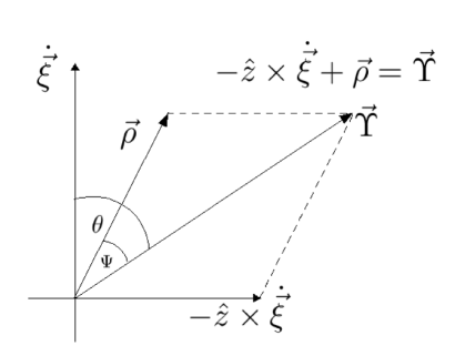
Figure 1: An illustrative picture is shown for the angle $\Psi$. In addition, other parameters related to the geometry and the orientation of the dipole are depicted.

In addition, in the Figure (1), angle $\Psi$, dimensionless relative variable and the velocity of the center of mass are depicted at fixed time. Several parameters related to the geometry and the orientation of the dipole are shown.

III.1 Bound states

According to previous considerations, we know that the effective potential is a periodic function of the angle $\Psi$. If the energy $\varepsilon$ of the system lives between two extreme values, $V_{eff}^{min}=\left((1-\Upsilon)^{2}-\varepsilon_{c}\right)$ and $V_{eff}^{max}=\left((1+\Upsilon)^{2}-\varepsilon_{c}\right)$, the motion is bounded by two turning points. The value of total energy in such point $\varepsilon=V_{eff}(\rho)$ gives the limit of the oscillation.

Hence, from the Eq.(21) and by considering that $\dot{\vec{\rho}}\cdot\hat{\Psi}=d{\Psi}/d\tau$, we obtain by direct integration

$$\Delta\tau(\Psi)=\tau(\Psi)-\tau(\Psi_{0})=\frac{1}{2}\int_{\Psi_{0}}^{\Psi}\frac{d\Psi^{\prime}}{[\varepsilon+\varepsilon_{c}-1-{\Upsilon}^{2}+2\Upsilon\cos\Psi^{\prime}]^{1/2}},$$ (22)

where $\tau=\omega_{c}t$, which we write in terms of an incomplete elliptic integral of the first kind as follows

$$\Delta\tau(\Psi)=\frac{1}{2}F\left[\arcsin\left(\frac{\sin\Psi/2}{\sin\Psi_{\varepsilon}/2}\right)\setminus\frac{\Psi_{\varepsilon}}{2}\right]$$ (23)

where $\tau=\omega_{c}t$

The typical oscillation of the variable $\Psi$ for bound states represents a bound rotation between two limiting angles, $\pm\Psi_{\varepsilon}$, the classical turning points. That limiting angles are given by

$$\Psi_{\varepsilon}=\arccos(\frac{\varepsilon+\varepsilon_{c}-{\Upsilon}^{2}-1}{2\Upsilon}),$$ (24)

From the Eq.(18), the energy of the system determines the amplitude of the the oscillation. According to the Eq.(10), if the dipole enters to the magnetic field without an angular relative velocity, then the energy only depends on the initial orientation of the dipole. From the Eq.(22) and the Eq.(24) the period of the motion can be given by

$$\tau_{P}=\frac{1}{\sqrt{2\Upsilon}}\int_{-\Psi_{\varepsilon}}^{\Psi_{\varepsilon}}\frac{d\Psi^{\prime}}{[\cos\Psi^{\prime}-\cos\Psi_{\varepsilon}]^{1/2}}.$$ (25)

Now, we use the definition of the complete elliptic integral of the first kind to write the period of the motion

$$\tau_{P}=\frac{2}{\sqrt{\Upsilon}}K\left[\sin\frac{\Psi_{\varepsilon}}{2}\right].$$ (26)

In addition, we can use the definition of the hypergeometric functionArfken to present the same, as follows,

$$\tau_{P}=\pi\frac{1}{\sqrt{\Upsilon}}\;\;\;{}_{2}{\cal{F}}_{1}\left[\frac{1}{2},\frac{1}{2},\sin\frac{\Psi_{\varepsilon}}{2}\right].$$ (27)

Using the approximation of small oscillations, i.e., for energies near to the point of the stable equilibrium $V_{ef}^{min}$, the dimensionless frequency $\omega_{P}$ is given by

$$\omega_{P}=\frac{\sqrt{\Upsilon}}{2}$$ (28)

Clearly, this frequency depends on $\Upsilon$, which corresponds to the initial orientation and the initial velocity of the center of mass from the Eq.(11).

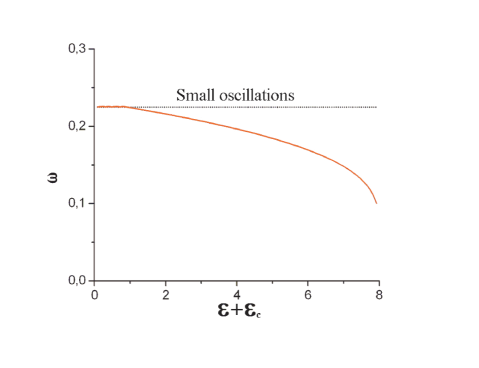
Figure 2: The frequency is depicted as a function of energy $\varepsilon+\varepsilon_{c}$. The exact value for the frequency coincides with the value in the aproximation of small oscillations in the limit $\varepsilon\rightarrow-\varepsilon_{c}$

In the Figure 2 is depicted the relation between the dimensionless frequency and the dimensionless energy. In the approximation of small oscillations, we can get the effective potential as a quadratic function of the angle $\Psi$. This is, the period of such oscillations is independent of its amplitude. The exact value for the frequency $\omega$ for $\varepsilon+\varepsilon_{c}\rightarrow 0$ approaches to the analytical value for the frequency $\omega_{P}$ from small oscillations.

III.2 Trapped States

The classical trapped states are defined when the mean value of the center of mass velocity is zero. From Eq.(16) we obtain

$$\langle\dot{\vec{\xi}}\rangle=\frac{1}{\tau}\int_{0}^{\tau}d\tau^{\prime}(-\hat{z}\times\vec{\rho}+\hat{z}\times\vec{\Upsilon})=0$$ (29)

where $\tau$ is the dimensionless period. The present condition represents a closed motion. We expect to characterize a family of unbounded states, without classical turning points, which can satisfy the previous restriction. By following, we write by compounds,

$$\langle\dot{\vec{\xi_{\parallel}}}\rangle = -\frac{1}{\tau}\int_{0}^{\tau}d\tau^{\prime}\cos\theta=0$$ (30)

$$\langle\dot{\vec{\xi_{\perp}}}\rangle = \frac{1}{\tau}\int_{0}^{\tau}d\tau^{\prime}(-\sin\theta+\Upsilon)=0,$$ (31)

where $\theta$ is the angle between $\dot{\vec{\xi}}$ and $\vec{\Upsilon}$ (see Figure 1) and the symbols $\dot{\vec{\xi_{\parallel}}}$ and $\dot{\vec{\xi_{\perp}}}$ are referred to the parallel and perpendicular parts of $\dot{\vec{\xi}}$ respecting to the vector $\vec{\Upsilon}$. Furthermore, we take into account that $\vec{\Upsilon}=\Upsilon\hat{\Upsilon}$, where $\hat{\Upsilon}$ is a unit vector. We see that if $\Upsilon=0$, Eq.(30) and Eq.(31) are simply satisfied, the classical motion is trapped for any dimensionless energy $\varepsilon>1-\varepsilon_{c}$, , we obtain from Eq.(21) the frequency of the trapped state that is given by $\dot{\Psi}=2\sqrt{\varepsilon+\varepsilon_{c}-1}$. In addition, we can emphasize that if $\Upsilon\neq 0$, Eq.(30) is always satisfied; however, the Eq.(31) imposes that $-1\leq\Upsilon\leq 1$, while if $|{\Upsilon}|>1$ the trapping should not be possible.

IV Summary

We have proposed to introduce a description of the classical dynamics of rotors such as electric dipoles in an external magnetic field. Our treatment does not consider radiation effects; however, the solution is nontrivial; therefore, we believe the present discussion would be pedagogically useful as a special topic of a standard course of classical mechanics.

In the present application, we have considered the motion in a perpendicular plane to a uniform magnetic field. The motion axis coincides with the direction of the magnetic field. We find the equations and constants of motion through the Lagrangian formulation in the symmetric gauge. Our results are conveniently presented in dimensionless variables. In the present view, bound states are obtained for a periodic potential with initial conditions, which satisfy Eq.(16) and Eq.(17). We are able to write a simple expression for the frequency of motion, $\omega_{P}=\sqrt{\Upsilon}/{2}$, in the approximation of small oscillations. Trapped motion is obtained as a particular case of the motion of the center of mass with an additional restriction, which satisfy Eq.(29), where there are no turning points. The definition of trapped states leads to a special range of values of the constant of motion, this is $|{\Upsilon}|<1$.

References

- (1) Hernández J V, Kay E R and Leigh D A 2004 A Reversible Synthetic Rotary Molecular Motor Science 306 1532-1536
- (2) Gimzewski J K, Joachim C, Schlittler R R, Langlais V, Tang H and Johansen I 1998 Rotation of a Single Molecule Within a Supramolecular Bearing Science 281 531-533
- (3) Bermudez V, Capron N, Gase T, Gatti F G, Kajzar F, Leigh D A, Zerbetto F and Zhang S 2000 Influencing intramolecular motion whith an alternating electric field Nature 406 608-611
- (4) Yurke B, Turberfield A J, Mills A P, Simmel F C and Neumann J L 2000 A DNA-fuelled molecular machine made of DNA Nature 406 605-608
- (5) Kelly T R, De Silva H and Silva R A 1999 Unidirectional rotary motion in a molecular system Nature 401 150-152
- (6) Koumura N, Zijlstra R W J, van Delben R A, Harada N and Feringa B L 1999 Light-driven monodirectional molecular rotor Nature 401 152-154
- (7) Guimarães P and Oliveira I S 1999 Classical and Quantum Mechanics of a Charged Particle in Oscillating Electric and Magnetic Fields, Braz. J. of Phys. 29 541-546
- (8) Spavieri G 1999 Quantum effect for an electric dipole Phys. Rev. A 59 3194-3199
- (9) Curilef S and Claro F 1997 Dynamics of two interacting particles in a magnetic field in two dimensions Am. J. Phys. 65 244-250
- (10) Truong T and Bazzali D 2000 Exact low-lying states of two interacting equally charged particles in a magnetic field Phys. Lett. A 269 186-193
- (11) Taut M 1999 Two particles whit opposite charge in a homogeneous magnetic field: particular analytical solutions of the two-dimensional Schrodinger equation J. Phys A: Math. Gen. 32 5509-5515
- (12) Pursey D L, Sveshnikov N A, Shirokov A M 1998 Electric dipole in a magnetic field: Bound states without classical turning points Theor. and Math. Phys. 117, 1262-1273
- (13) Arfken G B and Weber H J 2001 Mathematical Methods for Physicists, Fifth Edition, Academic Press