Seismic motion in urban sites consisting of blocks in welded contact with a soft layer overlying a hard half space: I. Finite set of blocks

Abstract

We address the problem of the response to a seismic wave of an urban site consisting of $N$ non-identical, non-equispaced blocks overlying a soft layer underlain by a hard substratum. The results of a theoretical analysis, appealing to a space-frequency mode-matching (MM) technique, are compared to those obtained by a space-time finite element (FE) technique. The two methods are shown to give rise to the same prediction of the seismic response for $N=1$ and $N=2$ blocks. The mechanism of the interaction between blocks and the ground, as well as that of the mutual interaction between blocks, are studied. It is shown that the presence of a small number of blocks modifies the seismic disturbance in a manner which evokes qualitatively, but not quantitatively, what was observed during the 1985 Michoacan earthquake in Mexico City. Disturbances at a much greater level, induced by a large number of blocks (in fact, a periodic set) are studied in the companion paper.

Keywords: Duration, amplification, seismic response, cities.

Abbreviated title: Seismic response in urban sites

Corresponding author: Armand Wirgin, tel.: 33 4 91 16 40 50, fax: 33 4 91 16 42 70
e-mail: wirgin@lma.cnrs-mrs.fr

1 Introduction

The Michoacan earthquake that struck Mexico City in 1985 presented some particular characteristics which have since been encountered at various other locations [41, 42, 27, 34, 25], but at a lower level of intensity. Other than the fact that the response in downtown Mexico varied considerably in a spatial sense [15], was quite intense and of very long duration at certain locations (as much as $\approx$3min [38]), and often took the form of a quasi-monochromatic signal with beatings [36], a remarkable feature of this earthquake (studied in [16, 6, 21, 22]) was that such strong motion could be caused by a seismic source so far from the city (the epicenter was located in the subduction zone off the Pacific coast, approximately 350km from Mexico City). It is now recognized [6, 7] that the characteristics of the abnormal response recorded in downtown Mexico were partially present in the waves entering into the city (notably $60$km from the city as recorded by the authors of [16]) after having accomplished their voyage from the source, this being thought to be due to the excitation of Love and generalized-Rayleigh modes by the irregularities of the crust [6, 9, 16]).

In the present investigation (as well as in the companion paper), we focus on the influence of the presence of the built features of the urban site as a complementary explanation of the abnormal response: the so-called city-site effect. A building or a group of buildings over a hard half-space, solicited by a plane incident SH wave, has been shown to modify the seismic waves on the ground near the building [46, 33], the modification being larger when more buildings are taken into account because of multiple-interaction: i.e., the so-called structure-soil-structure interaction. For models of the geophysical structure involving only a hard half-space, the stress-free base block mode appears to be the main cause of the modification [33].

The studies that deal with a geophysical structure involving, in addition, a soft-layer overlying the hard-half space, have been mainly concerned either with an infinite set of periodically-arranged [2, 4, 5] or randomly- arranged [32, 10] buildings on, or partially imbedded in, the ground. In [2], the authors suggest that the large duration and amplitude are strongly linked to resonant phenomena of the soft-layer associated with waves whose structure is close to that of Love waves. The solicitation being of the form of a plane incident wave, such modes cannot be excited in the absence of buildings [21].

In [31, 26], it was shown that the modes of a soft layer/hard half space can be excited when the interface between the subtratum and the layer present some irregularities. These effects were qualified as ”vertical and lateral interferences” in a previous numerical study [1]. The question of the excitation of modes, via surface irregularities constituted by the set of buildings on the ground, was subsequently addressed in [19]. In [49, 48] it was found that the excitation of vibration modes associated with a periodically-modulated surface impedance, modeling a periodic distribution of blocks emerging from a flat ground, can lead to enhanced durations and amplifications of the cumulative displacement and velocity as compared to what is found for a flat stress-free or constant surface impedance surface. The authors of [48] show that these modes manifest themselves by amplified evanescent waves in the substratum.

The contributions [4, 5] employ homogeneized models of a periodic city, but the fact that these models are restricted to low frequencies may explain why they do not account for the amplifications obtained in [19] [48]. In a host of other numerical studies [32, 24, 8, 4, 5, 10, 13, 14], the presence of buildings is found either to hardly modify, or to de-amplify, the seismic disturbance, in contradiction with what is shown in [43, 47, 17].

In [39], the spatial variability of damage to structures on the ground was attributed to the variability of the resonance frequencies of the buildings and of the soil structure beneath each building, with the implication that the most dangerous situation is when the natural frequency of the building (often treated as a one degree (or several degrees) of freedom oscillator [29, 23, 10, 5, 40]) is coincident with that (obtained by a 1D analysis) of the substructure below the base of the building (a well-known paradigm in the civil engineering community known as the double resonance).

Another point of view is to consider the building as a seismic source, either when it is solicited artificially by a vibrator located on its roof [28, 50], or when it re-emits vibrations received from the incident seismic disturbance (or other form of solicitation such as that coming from an underground nuclear explosion [44, 12]). It is not unreasonable to think that the presence of one or more buildings on the ground enables the excitation of the (Love, Rayleigh) modes of the underground system. This is known to be possible when a flat stress-free surface overlying a soft layer in welded contact with a hard substratum is solicited by a source located in the layer or substratum [21] and should therefore also occur when the source (i.e., the building) is on the free surface.

The present work originated in the observation that no satisfactory theoretical explanation has been given until now of the influence of buildings on anomalous seismic response in urban environments with soft layers, or large basins, overlying a hard substratum. The principal reason for this knowledge gap probably lies in the complexity of the sites examined in previous studies and in the complexity of the phenomena. Thus, it appears to be opportune to develop a theoretical model which is as complete and as simple as possible, on an idealized, although rather representative urban site, in order to address the following questions:

(i) how should one account for the principal features of the seismic response in the cases of a relatively small, and then, large number of blocks?

(ii) what are the modes of the global structures (i.e. the superstructure plus the geophysical structure) and what are the mechanisms of their excitation and interaction?

(iii) what are the repercussions of resonant phenomena on the seismic response?

(iv) what are the differences in seismic response between configurations with a small and a large number of blocks?

The investigation herein focuses on the seismic response of one and two blocks (the case of a periodic set of blocks is considered in the companion parper) in welded contact with a soft layer overlying a hard half-space. The modal analysis of the whole configuration, backed up by extensive numerical computations, shows that: i) the presence of one block induces the excitation of two types of modes, the first whose structure is close to that of a mode of the geophysical structure, and the second whose structure is close to that of a mode of the superstructure (i.e., the set of blocks, each of which is formed of one or several buildings), ii) the presence of more than one block gives rise to coupled modes resulting from a combination of the two other types of modes.

We uncover the mechanism of the (so-called soil-structure) interaction between the superstructure and the geophysical substructure. Despite the fact that differences are noticed between the computed displacements for a configuration with, and in the absence of, buildings, mainly consisting in a longer duration and a larger displacement in the building than at the same location in the absence of the building, and in a modification, due to the presence of the block(s) of the structure of the waves traveling in the layer, no very pronounced effects are apparent in the case of only a few (one or two) buildings. This could mean that the city-site effect is important only when a large number of buildings is accounted for. This case is investigated theoretically and numerically in the companion paper for a periodic arrangement of identical blocks.

2 Description of the configuration

We focus on a portion of a modern city consisting of a set of blocks (see e.g., fig. 1 in which it will be noted that the blocks (i.e., buildings or groups of buildings) are not generally identical, nor arranged in periodic manner). The city has 2D geometry, with $x_{3}$ the ignorable coordinate of a $Ox_{1}x_{2}x_{3}$ cartesian coordinate system (see Fig. 2).

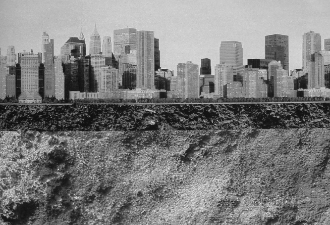
Figure 1: View of a modern city with the underground.

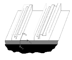
Figure 2: View of the 2D city (only two of the blocks are represented).

The buildings are assumed to be in welded contact, across the flat ground surface, with the substructure. The latter is composed of a horizontal soft layer underlain by a hard half space (see fig. 1). Each block is characterized by two constants, its height $b_{j}$ and width $w_{j}$, and all blocks have the same rectangular geometry (but not the same sizes) and composition. Let $d_{j}$ be the $x_{1}$ coordinate of the center of the base segment of the $j-$th block. The distance between the blocks $j$ and $i$ is denoted by $d_{ji}=|d_{j}-d_{i}|$ and is not necessarily constant between successive pairs of blocks.

For the purpose of analysis, each block is homogenized (this does not mean that the set of blocks is reduced to a single horizontal, homogeneous layer, as in [4, 5]), so that the final aspect of the city is as in Fig. 3.

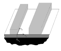
Figure 3: View of the 2D city with homogenized blocks (only two of the blocks are represented).

Let $\mathbb{B}\in\mathbb{Z}$ denote the set of indices by which the blocks are identified (e.g., for three blocks: $\{1,2,3\}$ or $\{-1,0,1\}$). The cardinal of $\mathbb{B}$ is designated by $N$ (i.e., $N$ denotes the number of blocks in the configuration, and this number will either be finite (in the following analysis) or infinite (as in the companion paper).

$\Gamma_{f}$ is the stress-free surface composed of a ground portion $\Gamma_{g}$, assumed to be flat and horizontal, and a portion $\Gamma_{ag}$, constituting the reunion of the above-ground-level boundaries $\Gamma_{ag}^{j}~{};~{}j\in\mathbb{B}$ of the blocks. The ground $\Gamma_{G}$ is flat and horizontal, and is the reunion of $\Gamma_{g}$ and the base segments $\Gamma_{bs}^{j}~{};~{}j\in\mathbb{B}$ joining the blocks to the underground.

The medium in contact with, and above, $\Gamma_{f}$ is air, assumed to be the vacumn (which is why $\Gamma_{f}$ is stress-free). The medium in contact with, and below $\Gamma_{G}$ is the mechanically-soft layer occupying the domain $\Omega_{1}$, which is laterally-infinite and of thickness $h$, and whose lower boundary is $\Gamma_{h}$, also assumed to be flat and horizontal. The soft material in the layer is in welded contact across $\Gamma_{h}$ with the mechanically-hard material in the semi-infinite domain (substratum) $\Omega_{0}$.

The domain of the $j$-th block is denoted by $\Omega_{2}^{j}$ and the reunion of all the $\Omega_{2}^{j}~{};~{}j\in\mathbb{B}$ is denoted by $\Omega_{2}$. The material in each block is in welded contact with the material in the soft layer across the base segments $\Gamma_{bs}^{j}~{};~{}j\in\mathbb{B}$.

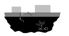
Figure 4: Sagittal ($x_{1}0x_{2}$) plane view of the 2D city with homogenized blocks (only two of the blocks are represented) solicited by a cylindrical wave radiated by a line source located at $(x_{1}^{s},x_{2}^{s})\in\Omega_{0}$.

Figure 5: Sagittal ($x_{1}0x_{2}$) plane view of the 2D city with homogenized blocks (only two of the blocks are represented) solicited by a plane wave with incident angle $\theta^{i}$.

The origin $O$ of the cartesian coordinate system is on the ground, $x_{2}$ increases with depth and $x_{3}$ is perpendicular to the (sagittal) plane of the figs. 4-5. With $\mathbf{i}_{j}$ the unit vector along the positive $x_{j}$ axis, we note that the unit vectors normal to $\Gamma_{G}$ and $\Gamma_{h}$ are $-\mathbf{i}_{2}$.

The media filling $\Omega_{0}$, $\Omega_{1}$ and $\bigcup_{j\in\mathbb{B}}\Omega_{2}^{j}$ are $M^{0}$, $M^{1}$ and $M^{2}$ respectively and the latter are assumed to be initially stress-free, linear, isotropic and homogeneous (thus, each block, which is generally inhomogeneous, is assumed to be homogenized in our analysis). We assume that $M^{0}$ is non-dissipative whereas $M^{1}$ and $M^{2}$ are dissipative, described by a constant quality factor $Q^{j}$ in the frequency range of excitation.

The seismic disturbance is delivered to the site in the form of a shear-horizontal (SH) cylindrical wave (radiated by a line source parallel to the $x_{3}$ axis and located in $\Omega_{0}$; see fig. 4) or a plane wave (with incident angle $\theta^{i}$; see fig. 5), propagating initially in $\Omega_{0}$ (this meaning, that in the absence of the layer, the city, and the air, the total field is precisely that associated with this cylindrical or plane wave). The SH nature of the incident wave (indicated by the superscript $i$ in the following) means that the motion associated with it is strictly transverse (i.e., in the $x_{3}$ direction and independent of the $x_{3}$ coordinate). Both the SH polarization and the invariance of the incident wave with respect to $x_{3}$ are communicated to the fields that are generated at the site in response to the incident wave. Thus, our analysis deals with the propagation of 2D SH waves (i.e., waves that depend exclusively on the two cartesian coordinates $(x_{1},x_{2})$ and that are associated with motion in the $x_{3}$ direction only).

We shall be concerned with a description of the elastodynamic wavefield on the free surface (i.e., on $\Gamma_{f}$) resulting from the cylindrical or plane seismic wave sollicitation of the site.

3 Governing equations

3.1 Space-time framework wave equations

In a generally-inhomogeneous, isotropic elastic or viscoelastic medium $M$ occupying $\mathbb{R}^{3}$, the space-time framework wave equation for SH waves is:

$$\nabla\cdot(\mu(\mathbf{x},\omega)\nabla u(\mathbf{x},t))-\rho(\mathbf{x})\partial_{t}^{2}u(\mathbf{x},t)=-\rho(\mathbf{x})f(\mathbf{x},t)~{},$$ (1)

wherein $u$ is the displacement component in the $\mathbf{i}_{3}$ direction, $f$ the component of applied force density in the $\mathbf{i}_{3}$ direction, $\mu$ the Lamé descriptor of rigidity, $\rho$ the mass density, $t$ the time variable, $\omega$ the angular frequency, $\partial^{n}_{t}$ the $n-$th partial derivative with respect to $t$, and $\mathbf{x}=(x_{1},x_{2})$. Since our configuration involves three homogeneous media, and the applied force is assumed to be non vanishing only in $\Omega_{0}$, we have

$$\left(c^{m}(\omega)\right)^{2}\nabla\cdot\nabla u^{m}(\mathbf{x},t)-\partial_{t}^{2}u^{m}(\mathbf{x},t)=-f(\mathbf{x},t)\delta_{m0}~{}~{};~{}~{}\mathbf{x}\in\Omega_{m}~{};~{}m=0,1,2~{},$$ (2)

wherein superscripts $m$ designate the medium (0 for $M^{0}$, etc.), $\delta_{m0}=1$ for $m=0$, $\delta_{m0}=0$ for $m\neq 0$, and $c^{m}$ is the generally-complex velocity of shear body waves in $M^{m}$, related to the density and rigidity by

$$\left(c^{m}(\omega)\right)^{2}=\frac{\mu^{m}(\omega)}{\rho^{m}}~{},$$ (3)

it being understood that $\rho^{m},~{}\mu^{m}(\omega)~{};~{}m=0,1,2$ are constants with respect to $\mathbf{x}$. In addition, the densities are positive real and we assume that substratum is a dissipation-free solid so that the rigidity therein is a positive real constant with respect to $\omega$, i.e., $\mu^{0}(\omega)=\mu^{0}>0$.

3.2 Space-frequency framework wave equations

The space-frequency framework versions of the wave equations are obtained by expanding the force density and displacement in Fourier integrals:

$$f(\mathbf{x},t)=\int_{-\infty}^{\infty}f(\mathbf{x},\omega)e^{-\mbox{i}\omega t}d\omega~{}~{},~{}~{}u^{m}(\mathbf{x},t)=\int_{-\infty}^{\infty}u^{m}(\mathbf{x},\omega)e^{-\mbox{i}\omega t}d\omega~{},\forall t\in\mathbb{R}~{},$$ (4)

so as to give rise to the Helmholtz equations

$$\nabla\cdot\nabla u^{m}(\mathbf{x},\omega)+\left(k^{m}(\omega)\right)^{2}u^{m}(\mathbf{x},\omega)=-f(\mathbf{x},\omega)\delta_{m0}~{}~{};~{}~{}\forall\mathbf{x}\in\Omega_{m}~{}~{};~{}~{}m=0,1~{},$$ (5)

wherein

$$k^{m}(\omega):=\frac{\omega}{c^{m}(\omega)}=\omega\sqrt{\frac{\rho^{m}}{\mu^{m}(\omega)}}~{}.$$ (6)

is the generally-complex wavenumber in $M^{m}$. Actually, due to the assumptions made in sects. 2 and 3.2:

$$k^{0}(\omega):=\frac{\omega}{c^{0}}=\omega\sqrt{\frac{\rho^{0}}{\mu^{0}}}~{},$$ (7)

(i.e., $k^{0}$ is a positive real quantity which depends linearly on $\omega$ ).

As mentioned above, we shall be concerned with cylindrical or plane wave excitation of the city. Plane waves correspond to $f=0$ and cylindrical waves to $f\neq 0$.

The incident field is chosen to take the form of a pseudo Ricker-type pulse in the time domain.

3.3 Space-frequency framework expression of the driving force for cylindrical wave excitation

The space-frequency framework expression of the driving force density for a cylindrical wave radiated from a line source located at $\mathbf{x}^{s}:=(x_{1}^{s},x_{2}^{s})\in\Omega_{0}$ is

$$f(\mathbf{x},\omega)=S(\omega)\delta(\mathbf{x}-\mathbf{x^{s}})~{},$$ (8)

wherein $S(\omega)$ is the spectrum of the incident pulse and is chosen to be a time derivative of a Ricker pulse and $\delta(.)$ is the Dirac distribution. The amplitude spectrum $S(\omega)$ is given by

$$S(\omega)=\frac{12\pi\alpha^{2}\omega^{2}}{\sqrt{\pi}}\frac{\omega^{2}}{4\alpha^{3}}\exp\left(\mbox{i}t_{s}\omega-\frac{\omega^{2}}{4\alpha^{2}}\right)~{},$$ (9)

to which corresponds the temporal variation (Fourier inverse of $S(\omega)$):

$$S(t)=-24\pi\alpha^{4}\left[-3(t_{s}-t)+2\alpha^{2}(t_{s}-t)^{3}\right]\exp\left[-\alpha^{2}(t_{s}-t)^{2}\right]~{},$$ (10)

wherein $\alpha=\pi/t_{p}$, $t_{p}$ is the characteristic period of the pulse, and $t_{s}$ the time at which the pulse attains its maximal value. In the remainder of this paper, we shall take $t_{s}=t_{p}=2$ sec.

The (incident) wave associated with this driving force is

$$u^{i}(\mathbf{x},\omega)=\int_{\mathbb{R}^{2}}G^{0}(\|\mathbf{x}-\mathbf{y}\|,\omega)f(\mathbf{y},\omega)d\varpi(\mathbf{y})~{},$$ (11)

wherein $\mathbf{y}:=(y_{1},y_{2})$ is an integration point in the sagittal plane, $d\varpi(\mathbf{y})$ the differential area element at point $\mathbf{y}$ and $G^{0}(k^{0}\|\mathbf{x}-\mathbf{y}\|)$ the 2D free-space Green’s function which satisfies:

$$\left[\Delta+\left(k^{0}\right)^{2}\right]G^{0}(\|\mathbf{x}-\mathbf{y}\|,\omega)=-\delta(\mathbf{x}-\mathbf{y})~{};~{}\forall\mathbf{x}\in\mathbb{R}^{2}~{},$$ (12)

(with $\delta(~{}.~{})$ the Dirac delta distribution) and the (outgoing wave) radiation condition:

$$G^{0}(\|\mathbf{x}-\mathbf{y}\|,\omega)\sim~{}\text{ outgoing waves}~{}~{};~{}~{}\|\mathbf{x}-\mathbf{y}\|\rightarrow\infty~{}.$$ (13)

The free-space Green’s function is given by [37]:

$$G^{0}(\|\mathbf{x}-\mathbf{y}\|,\omega)=\frac{\mbox{i}}{4}H_{0}^{(1)}(k^{0}\|\mathbf{x}-\mathbf{y}\|)=\frac{\mbox{i}}{4\pi}\int_{-\infty}^{\infty}\exp\{i[k_{1}(x_{1}-y_{1})+k_{2}^{0}|x_{2}-y_{2}|]\}\frac{dk_{1}}{k_{2}^{0}}~{},$$ (14)

with $H_{0}^{(1)}(.)$ the Hankel function of the first kind and order $0$, and

$$k_{2}^{j}=\sqrt{(k^{j})^{2}-(k_{1})^{2}}~{}~{};~{}~{}\Re k_{2}^{j}\geq 0~{}~{},~{}~{}\Im k_{2}^{j}\geq 0~{}~{}\text{for}~{}\omega\geq 0~{}.$$ (15)

Introducing (14) and (9) into (11) results in

$$u^{i}(\mathbf{x},\omega)=S(\omega)G^{0}(\|\mathbf{x}-\mathbf{x}^{s}\|,\omega)=S(\omega)\frac{\mbox{i}}{4}H_{0}^{(1)}(k^{0}\|\mathbf{x}-\mathbf{x}^{s}\|)~{},$$ (16)

which is the space-frequency expression of a cylindrical wave.

3.4 Material constants in a dissipative medium

A word is now in order concerning the dissipative nature of the layer and blocks. In seismological applications involving viscoelastic media, the quality factor is usually considered to be either constant or a weakly-varying function of frequency [13] in the bandwith of the source. We shall therefore assume that $Q^{j}(\omega)=Q^{j}$, with $Q^{j}$ constants, $j=1,2$. It can be shown [30] that this implies

$$\mu^{j}(\omega)=\mu^{j}_{ref}\left(\frac{-\mbox{i}\omega}{\omega_{ref}}\right)^{\frac{2}{\pi}\arctan\left(\frac{1}{Q^{j}}\right)}~{};~{}j=1,2~{},$$ (17)

wherein: $\omega_{ref}$ is a reference angular frequency, chosen herein to be equal to $9\times 10^{-2}$Hz. Hence

$$c^{j}(\omega)=c^{j}_{ref}\left(\frac{-\mbox{i}\omega}{\omega_{ref}}\right)^{\frac{1}{\pi}\arctan\left(\frac{1}{Q^{j}}\right)}~{};~{}j=1,2~{},$$ (18)

with $c^{j}_{ref}:=\sqrt{\frac{\mu^{j}_{ref}}{\rho^{j}}}$. Note should be taken of the fact that even though $Q^{j}~{},~{}j=1,2$ are non-dispersive (i.e., do not depend on $\omega$) under the present assumption, the phase velocities $c^{j}~{};~{}j=1,2$ are dispersive.

3.5 Boundary and radiation conditions in the space-frequency framework

The translation of the stress-free (i.e., vanishing traction) nature of $\Gamma_{f}=\Gamma_{g}\bigcup\Gamma_{ag}$, with $\Gamma_{ag}:=\bigcup_{j\in\mathbb{B}}\Gamma_{ag}^{j}$, is:

$$\mu^{1}(\omega)\partial_{n}u^{1}(\mathbf{x},\omega)=0~{};~{}\mathbf{x}\in\Gamma_{g},$$ (19)

$$\mu^{2}(\omega)\partial_{n}u^{2(j)}(\mathbf{x},\omega)=0~{};~{}\mathbf{x}\in\Gamma_{ag}^{j}~{},~{}j\in\mathbb{B}$$ (20)

wherein $\mathbf{n}$ denotes the generic unit vector normal to a boundary and $\partial_{n}$ designates the operator $\partial_{n}=\mathbf{n}\cdot\nabla$.

That $M^{1}$ and $M^{2}$ are in welded contact across $\Gamma_{bs}:=\bigcup_{j\in\mathbb{B}}\Gamma_{bs}^{j}$ is translated by the fact that the displacement and traction are continuous across $\Gamma_{bs}$:

$$u^{1}(\mathbf{x},\omega)-u^{2(j)}(\mathbf{x},\omega)=0~{};~{}\mathbf{x}\in\Gamma_{bs}^{j}~{},~{}j\in\mathbb{B}$$ (21)

$$\mu^{1}(\omega)\partial_{n}u^{1}(\mathbf{x},\omega)-\mu^{2}(\omega)\partial_{n}u^{2(j)}(\mathbf{x},\omega)=0~{};~{}\mathbf{x}\in\Gamma_{bs}^{j}~{},~{}j\in\mathbb{B}.$$ (22)

That $M^{1}$ and $M^{0}$ are in welded contact across $\Gamma_{h}$ is translated by the fact that the displacement and traction are continuous across this interface:

$$u^{1}(\mathbf{x},\omega)-u^{0}(\mathbf{x},\omega)~{};~{}\mathbf{x}\in\Gamma_{h}~{},$$ (23)

$$\mu^{1}(\omega)\partial_{n}u^{1}(\mathbf{x},\omega)-\mu^{0}(\omega)\partial_{n}u^{0}(\mathbf{x},\omega)~{};~{}\mathbf{x}\in\Gamma_{h}.$$ (24)

The uniqueness of the solution to the forward-scattering problem is assured by the radiation condition in the substratum:

$$u^{0}(\mathbf{x},\omega)-u^{i}(\mathbf{x},\omega)\sim~{}\text{ outgoing waves}~{}~{};~{}~{}\|\mathbf{x}\|\rightarrow\infty,~{}~{}x_{2}>h~{}.$$ (25)

3.6 Boundary and radiation conditions in the space-time framework

Since our finite element method [18, 19, 17] for solving the wave equation in a heterogeneous medium $M$ (in our case, involving three homogeneous components, $M^{0}$, $M^{1}$ and $M^{2}$) relies on the assumption that $M$ be a continuum, it does not appeal to any boundary conditions except on $\Gamma_{f}$ where the vanishing traction condition is invoked (fictitious domain method). Furthermore, since the essentially unbounded nature of the geometry of the city cannot be implemented numerically, we take this geometry to be finite and surround it (except on the $\Gamma_{f}$ portion) by a perfectly-matched layer (PML) [11] which enables closure of the computational domain without generating unphysical reflected waves (from the PML layer). In a sense, this replaces the radiation condition of the unbounded domain. The stress-free boundary condition on $\Gamma_{f}$ is modeled with the help of the fictitious domain method [3], which allows us to account for the diffraction of waves by a boundary of complicated geometry, not necessarily matching the volumic mesh.

3.7 Statement of the boundary-value (forward - scattering) problem in the space-time framework

The problem is to determine the time record of the displacement fields $u^{1}(\mathbf{x},t)$ on $\Gamma_{g}$ and $u^{2(j)}(\mathbf{x},t)$ on $\Gamma_{ag}^{j}$, $j\in\mathbb{B}$.

3.8 Recovery of the space-frequency displacements from the space-time displacements

The spectra of the displacements are obtained from the time records of the displacements by Fourier inversion, i.e.,

$$u^{j}(\mathbf{x},\omega)=\frac{1}{2\pi}\int_{-\infty}^{\infty}u^{j}(\mathbf{x},t)e^{\mbox{i}\omega t}dt~{};~{}j=1,2~{}.$$ (26)

4 Field representations in the space-frequency framework for $N<\infty$

4.1 Field in $\Omega_{0}$

It is useful to consider the boundary $\partial\Omega_{0}$ of $\Omega_{0}$ to be composed of $\Gamma_{h}$ plus a semi-circle of infinite radius $\Gamma_{\infty}$ joining $\Gamma_{h}$ at $\mathbf{x}=(-\infty,h)$ and $\mathbf{x}=(-\infty,h)$. The unit vector $\mathbf{n}$ normal to $\partial\Omega_{0}$ is taken to be outward with respect to $\Omega_{0}$, so that it is equal to $-\mathbf{i}_{2}$ on $\Gamma_{h}$.

We seek the field representation in $\Omega_{0}$. Applying Green’s second identity to $u^{0}$ and $G^{0}$ in $\Omega_{0}$ and making use of the radiation condition at infinity relative to these two functions, gives

$$\mathcal{H}_{\Omega_{0}}(\mathbf{x})u^{0}(\mathbf{x},\omega)=u^{i}(\mathbf{x},\omega)+\\ \int_{\Gamma_{h}}\left[G^{0}(\|\mathbf{x}-\mathbf{y}\|,\omega)\partial_{n}u^{0}(\mathbf{y},\omega)-u^{0}(\mathbf{y},\omega)\partial_{n}G^{0}(\|\mathbf{x}-\mathbf{y}\|,\omega)\right]d\gamma(\mathbf{y})~{},$$ (27)

wherein $d\gamma(\mathbf{y})$ is the infinitesimal arc length along $\Gamma_{h}$ and

$$\mathcal{H}_{\Omega_{0}}(\mathbf{x})=\left\{\begin{array}[]{cc}1&~{};~{}\mathbf{x}\in\Omega_{0}\\ 0&~{}~{}~{}~{}~{}~{}~{}~{};~{}\mathbf{y}\in\mathbb{R}^{2}\setminus\overline{\Omega}_{0}\\ 1/2&;~{}\mathbf{y}\in\Gamma_{h}\end{array}\right.~{}.$$ (28)

Introducing the cartesian coordinate integral representation of the Green’s function (14) into the boundary integral representation of the field (27), while paying attention to the absolute values, leads to the following result:

$$u^{0}(\mathbf{x},\omega)=u^{i}(\mathbf{x},\omega)+\int_{-\infty}^{\infty}B^{0}(k_{1},\omega)\exp\left\{\mbox{i}\left[k_{1}x_{1}+k_{2}^{0}(x_{2}-h)\right]\right\}\frac{dk_{1}}{k_{2}^{0}}~{};~{}\mathbf{x}\in\Omega_{0}~{},$$ (29)

wherein:

$$B^{0}(k_{1},\omega)=\frac{i}{4\pi}\int_{-\infty}^{\infty}\left\{\partial_{y_{1}}u^{0}(y_{1},h,\omega)+ik_{2}^{0}u^{0}(y_{1},h,\omega)\right\}\exp\left(-ik_{1}y_{1}\right)dy_{1}~{},$$ (30)

At this point, we must distinguish between plane wave excitation (briefly alluded-to in a subsequent section) and cylindrical wave excitation (to which all the following numerical results apply).

In the case of plane-wave excitation we can write

$$u^{i}(\mathbf{x},\omega)=\int_{-\infty}^{\infty}A^{0-}(k_{1},\omega)\exp\left\{i\left[k_{1}x_{1}-k_{2}^{0}x_{2}\right]\right\}\frac{dk_{1}}{k_{2}^{0}}~{};~{}\mathbf{x}\in\mathbb{R}^{2}~{},$$ (31)

wherein

$$A^{0-}(k_{1},\omega)=S(\omega)k_{2}^{0}\delta(k_{1}-k_{1}^{i})~{},$$ (32)

with $k_{1}^{i}=k^{0}\sin\theta^{i}$, and $\theta^{i}$ the angle of incidence, so that

$$u^{i}(\mathbf{x},\omega)=S(\omega)\exp\left\{\mbox{i}\left[k_{1}^{i}x_{1}-k_{2}^{i}x_{2}\right]\right\}~{};~{}\mathbf{x}\in\mathbb{R}^{2}~{},$$ (33)

wherein $k_{2}^{i}=k^{0}\cos\theta^{i}$.

In the case of cylindrical wave excitation, we have, on account of (14) and (16):

$$u^{i}(\mathbf{x},\omega)=\left\{\begin{array}[]{cc}\displaystyle\int_{-\infty}^{\infty}A^{0+}(k_{1},\omega)\exp\left\{\mbox{i}\left[k_{1}x_{1}+k_{2}^{0}x_{2}\right]\right\}\frac{dk_{1}}{k_{2}^{0}}&~{};~{}\mathbf{x}\in\Omega_{0}^{+}\\ \displaystyle\int_{-\infty}^{\infty}A^{0-}(k_{1},\omega)\exp\left\{\mbox{i}\left[k_{1}x_{1}-k_{2}^{0}x_{2}\right]\right\}\frac{dk_{1}}{k_{2}^{0}}&~{};~{}\mathbf{x}\in\Omega_{0}^{-}\end{array}\right.~{},$$ (34)

wherein

$$\Omega_{0}^{+}=\{\forall x_{1}\in\mathbb{R}~{};~{}x_{2}>x_{2}^{s}\}~{},$$ (35)

$$\Omega_{0}^{-}=\{\forall x_{1}\in\mathbb{R}~{};~{}h<x_{2}<x_{2}^{s}\}~{},$$ (36)

$$A^{0+}(k_{1},\omega)=S(\omega)\frac{\mbox{i}}{4\pi}\exp\left\{-\mbox{i}\left[k_{1}x_{1}^{s}+k_{2}^{0}x_{2}^{s}\right]\right\}~{},$$ (37)

$$A^{0-}(k_{1},\omega)=S(\omega)\frac{\mbox{i}}{4\pi}\exp\left\{-\mbox{i}\left[k_{1}x_{1}^{s}-k_{2}^{0}x_{2}^{s}\right]\right\}~{}.$$ (38)

Since we shall henceforth be interested only in the field in the subdomain $\Omega_{0}^{-}$ of $\Omega_{0}$, we can write

$$u^{0}(\mathbf{x},\omega)=\int_{-\infty}^{\infty}A^{0-}(k_{1},\omega)\exp\left\{\mbox{i}\left[k_{1}x_{1}-k_{2}^{0}x_{2}\right]\right\}\frac{dk_{1}}{k_{2}^{0}}+\\ \int_{-\infty}^{\infty}B^{0}(k_{1},\omega)\exp\left\{\mbox{i}\left[k_{1}x_{1}+k_{2}^{0}(x_{2}-h)\right]\right\}\frac{dk_{1}}{k_{2}^{0}}~{};~{}\mathbf{x}\in\Omega_{0}^{-}~{},$$ (39)

with the understanding that: i) $S(\omega)$ is known a priori and given by its expression in (9), ii) $A^{0\pm}(k_{1},\omega)$ are known a priori, iii) $B^{0}(k_{1},\omega)$ is an unknown function, iv) $A^{0\pm}(k_{1},\omega)$ and $B^{0}(k_{1},\omega)$ have units of (length) since $u^{0}$ (and, in general, all displacements), have units of length, v) $u^{0}$ is expressed as a sum of incoming and outgoing plane (bulk and evanescent) waves.

4.2 Field in $\Omega_{1}$

By proceeding in the same manner as previously we find

$$u^{1}(\mathbf{x},\omega)=\int_{-\infty}^{\infty}A^{1}(k_{1},\omega)\exp\left\{\mbox{i}\left[k_{1}x_{1}-k_{2}^{1}x_{2}\right]\right\}\frac{dk_{1}}{k_{2}^{1}}+\\ \int_{-\infty}^{\infty}B^{1}(k_{1},\omega)\exp\left\{\mbox{i}\left[k_{1}x_{1}+k_{2}^{1}x_{2}\right]\right\}\frac{dk_{1}}{k_{2}^{1}}~{};~{}\mathbf{x}\in\Omega_{0}~{},$$ (40)

with the understanding that: i) now both $A^{1}(k_{1},\omega)$ and $B^{1}(k_{1},\omega)$ are unknown functions, ii) $u^{1}$ is expressed as a sum of incoming and outgoing plane (bulk and evanescent) waves.

4.3 Field in the $j$-th block

The task is here to obtain a suitable representation of the field in the generic block $j$ (of height $b_{j}$ and width $w_{j}$) occupying the domain $\Omega_{2}^{j}$. The boundary of this domain is $\partial\Omega_{2}^{j}=\Gamma_{ag}^{j}\bigcup\Gamma_{bs}^{j}$. It should be recalled that the field satisfies a Neumann boundary condition on the emerged boundary $\Gamma_{ag}^{j}$ of the block. No boundary condition of the Neumann or Dirichlet type is available on the segment $\Gamma_{bs}^{j}$ so that, strictly speaking, we are not searching for a modal representation of the field in the block domain, but rather for a quasi-modal representation, the latter satisfying a priori the boundary condition on $\Gamma_{ag}^{j}$, but no particular boundary condition on $\Gamma_{bs}^{j}$.

Let $O^{j}x_{1}^{j}x_{2}^{j}x_{3}^{j}$ be the (local) cartesian coordinate system attached to $\Omega_{2}^{j}$ such that the origin $O^{j}$ is located on, and at the center of, the segment $\Gamma_{bs}^{j}$. We note that

$$x_{1}=d_{j}+x_{1}^{j}~{}~{},~{}~{}x_{2}=x_{2}^{j}~{}~{};~{}~{}\forall j\in\mathbb{B}~{},$$ (41)

wherein it should be recalled that $d_{j}$ is the $x_{1}$ coordinate of the center of the base segment of the $j-$th block.

We apply the separation of variables technique and the boundary conditions on $\partial\Omega_{2}^{j}$ to obtain

$$u^{2(j)}(\mathbf{x},\omega)=\sum_{m=0}^{\infty}B_{m}^{2(j)}(\omega)\cos\left[k^{2(j)}_{1m}\left(x_{1}^{j}+\frac{w_{j}}{2}\right)\right]\cos\left[k^{2(j)}_{2m}\left(x_{2}^{j}+b_{j}\right)\right]\\ ~{}~{};~{}~{}\mathbf{x}\in\Omega_{2}^{j}~{},~{}\forall j\in\mathbb{B}~{},$$ (42)

wherein

$$k^{2(j)}_{1m}=\frac{m\pi}{w_{j}}~{};~{}k^{2(j)}_{2m}=\sqrt{\left(k^{2}\right)^{2}-\left(k^{2(j)}_{1m}\right)^{2}}~{}~{};~{}~{}\Re\left(k^{2(j)}_{2m}\right)\geq 0~{}~{},~{}~{}\Im\left(k^{2(j)}_{2m}\right)\geq 0~{}~{}\text{for}~{}\omega\geq 0~{},$$ (43)

and $B_{m}^{2(j)}(\omega)$ has units of length. On account of (41) we finally obtain

$$u^{2(j)}(\mathbf{x},\omega)=\sum_{m=0}^{\infty}B_{m}^{2(j)}(\omega)\cos\left[k^{2(j)}_{1m}\left(x_{1}-d_{j}+\frac{w_{j}}{2}\right)\right]\cos\left[k^{2(j)}_{2m}\left(x_{2}+b_{j}\right)\right]\\ ~{}~{};~{}~{}\mathbf{x}\in\Omega_{2}^{j}~{},~{}\forall j\in\mathbb{B}~{},$$ (44)

it being understood that the $\mathbf{B}^{2(j)}:=\{B_{m}^{2(j)}(\omega)~{};~{}m\in\mathbb{Z}\}~{}~{},~{}~{}j\in\mathbb{B}$ are all unknown vectors.

5 Determination of the various unknown coefficients by application of boundary and continuity conditions on $\Gamma_{G}$ and $\Gamma_{h}$ for the case $N<\infty$

5.1 Application of the boundary and continuity conditions concerning the traction on $\Gamma_{G}$

From (20) and (21) we obtain

$$\mu^{1}\int_{-\infty}^{\infty}\partial_{x_{2}}u^{1}(x_{1},0,\omega)\exp(-\mbox{i}K_{1}x_{1})dx_{1}-\\ \mu^{2}\sum_{j\in\mathbb{B}}\int_{d_{j}-w/2}^{d_{j}+w/2}\partial_{x_{2}}u^{2(j)}(x_{1},0,\omega)\exp(-\mbox{i}K_{1}x_{1})dx_{1}=0~{}~{};~{}~{}\forall K_{1}\in\mathbb{R}~{}.$$ (45)

Introducing the appropriate field representations therein and making use of the orthogonality condition

$$\int_{-\infty}^{\infty}\exp[-\mbox{i}(k_{1}-K_{1})x_{1}]dx_{1}=2\pi\delta(k_{1}-K_{1})~{}~{};~{}~{}\forall k_{1}~{},~{}K_{1}\in\mathbb{R}~{},$$ (46)

gives rise to

$$A^{1}(k_{1},\omega)-B^{1}(k_{1},\omega)=\\ \frac{1}{2\pi\mbox{i}}\sum_{j\in\mathbb{B}}e^{-\mbox{i}k_{1}(d_{j}-w_{j}/2)}\sum_{m=0}^{\infty}B_{m}^{2(j)}(\omega)\frac{\mu^{2}k_{2m}^{2(j)}w_{j}}{\mu^{1}}I_{m}^{(j)-}(k_{1},\omega)\sin(k_{2m}^{2(j)}b_{j})~{}~{};~{}~{}\forall k_{1}\in\mathbb{R}~{},$$ (47)

wherein

$$I_{m}^{(j)\pm}(k_{1},\omega):=\int_{0}^{1}\exp(\pm\mbox{i}k_{1}w_{j}\eta)\cos(k_{1m}^{2(j)}w_{j}\eta)d\eta~{}.$$ (48)

5.2 Application of the continuity conditions concerning the displacement on $\Gamma_{G}$

From (22) we obtain

$$\int_{d_{l}-\frac{w}{2}}^{d_{l}+\frac{w}{2}}u^{1}(x_{1},0,\omega)\cos\left[k_{1n}^{2(l)}(x_{1}-d_{l}+w_{l}/2)\right]dx_{1}-\\ \int_{d_{l}-\frac{w}{2}}^{d_{l}+\frac{w}{2}}u^{2(l)}(x_{1},0,\omega)\cos\left[k_{1n}^{2(l)}(x_{1}-d_{l}+w_{l}/2)\right]dx_{1}=0~{}~{};~{}~{}\forall l\in\mathbb{B}~{}.$$ (49)

Introducing the appropriate field representations therein, and making use of the orthogonality condition

$$\int_{d_{l}-\frac{w}{2}}^{d_{l}+\frac{w}{2}}\cos\left[k_{1m}^{2(l)}(x_{1}-d_{l}+w_{l}/2)\right]\cos\left[k_{1n}^{2(l)}(x_{1}-d_{l}+w_{l}/2)\right]dx_{1}=\frac{w_{l}}{\epsilon_{m}}\delta_{mn}\\ ~{}~{};~{}~{}\forall m~{},~{}n=0,1,2,....~{},$$ (50)

wherein $\delta_{mn}$ is the Kronecker symbol and $\epsilon_{m}$ the Neumann symbol ($\epsilon_{m}=1$ for $m=0$, $\epsilon_{m}=2$ for $m>0$), gives rise to

$$B_{m}^{2(l)}(\omega)=\frac{\epsilon_{m}}{\cos(k_{2m}^{2(l)}b_{l})}\int_{-\infty}^{\infty}\left[A^{1}(k_{1},\omega)+B^{1}(k_{1},\omega)\right]I_{n}^{(l)+}(k_{1},\omega)e^{\mbox{i}k_{1}(d_{l}-w_{l}/2)}\frac{dk_{1}}{k_{2}^{1}}\\ ~{}~{};~{}~{}\forall m=0,1,2,....~{}~{},~{}~{}l\in\mathbb{B}~{}.$$ (51)

5.3 Application of the continuity conditions concerning the traction on $\Gamma_{h}$

From (23) we obtain

$$\mu^{0}\int_{-\infty}^{\infty}\partial_{x_{2}}u^{0}(x_{1},h,\omega)\exp(-\mbox{i}K_{1}x_{1})dx_{1}-\mu^{1}\int_{-\infty}^{\infty}\partial_{x_{2}}u^{1}(x_{1},h,\omega)\exp(-\mbox{i}K_{1}x_{1})dx_{1}=0~{}~{};~{}~{}\forall K_{1}\in\mathbb{R}~{}.$$ (52)

Introducing the appropriate field representations therein, and making use of the orthogonality relation (46), gives rise to

$$-\mu^{0}A^{0-}(k_{1},\omega)e^{-\mbox{i}k_{2}^{0}h}+\mu^{0}B^{0}(k_{1},\omega)+\mu^{1}A^{1}(k_{1},\omega)e^{-\mbox{i}k_{2}^{1}h}-\mu^{1}B^{1}(k_{1},\omega)e^{\mbox{i}k_{2}^{1}h}=0~{}~{};~{}~{}\forall k_{1}\in\mathbb{R}~{}.$$ (53)

5.4 Application of the continuity conditions concerning the displacement on $\Gamma_{h}$

From (24) we obtain

$$\int_{-\infty}^{\infty}u^{0}(x_{1},h,\omega)\exp(-\mbox{i}K_{1}x_{1})dx_{1}-\int_{-\infty}^{\infty}u^{1}(x_{1},h,\omega)\exp(-\mbox{i}K_{1}x_{1})dx_{1}=0~{}~{};~{}~{}\forall K_{1}\in\mathbb{R}~{}.$$ (54)

Introducing the appropriate field representations therein, and making use of the orthogonality relation (46), gives rise to

$$\frac{A^{0-}(k_{1},\omega)}{k_{2}^{0}}e^{-\mbox{i}k_{2}^{0}h}+\frac{B^{0}(k_{1},\omega)}{k_{2}^{0}}-\\ \frac{A^{1}(k_{1},\omega)e^{-\mbox{i}k_{2}^{1}h}}{k_{2}^{1}}-\frac{B^{1}(k_{1},\omega)e^{\mbox{i}k_{2}^{1}h}}{k_{2}^{1}}=0~{}~{};~{}~{}\forall k_{1}\in\mathbb{R}~{}.$$ (55)

5.5 Determination of the various unknowns

5.5.1 Elimination  of  $B_{m}^{2j}(\omega)$  to  obtain  an  integral equation for $B^{0}(k_{1},\omega)$

After a series of substitutions, the following integral equation for $B^{0}(k_{1},\omega)$ is obtained (wherein $K_{1}$ and $K_{2}^{j}$ play the same roles, and are related to each other in the same manner, as $k_{1}$ and $k_{2}^{j}$ respectively):

$$C(k_{1},\omega)B^{0}(k_{1},\omega)-\int_{-\infty}^{\infty}D(k_{1},K_{1},\omega)B^{0}(K_{1},\omega)dK_{1}=F(k_{1},\omega)~{}~{};~{}~{}\forall k_{1}\in\mathbb{R}~{},$$ (56)

wherein

$$C(k_{1},\omega)=\cos(k_{2}^{1}h)-\mbox{i}\frac{\mu^{1}k_{2}^{1}}{\mu^{0}k_{2}^{0}}\sin(k_{2}^{1}h)~{},$$ (57)

$$D(k_{1},K_{1},\omega)=\left[\cos(K_{2}^{1}h)-\mbox{i}\frac{\mu^{1}K_{2}^{1}}{\mu^{0}K_{2}^{0}}\sin(K_{2}^{1}h)\right]\times\\ \frac{i}{2\pi}\sum_{j\in\mathbb{B}}e^{\mbox{i}(K_{1}-k_{1})(d_{j}-w_{j}/2)}\sum_{m=0}^{\infty}\epsilon_{m}\frac{\mu^{2}k_{2m}^{2(j)}w_{j}}{\mu^{0}K_{2}^{0}}\tan(k_{2m}^{2(j)}b_{j})I_{m}^{(j)-}(k_{1},\omega)I_{m}^{(j)+}(K_{1},\omega)\\ ~{}~{};~{}~{}\forall k_{1},~{}K_{1}\in\mathbb{R}~{},$$ (58)

and

$$F(k_{1},\omega)=A^{0-}(k_{1},\omega)e^{-\mbox{i}k_{2}^{0}h}\left[\cos(k_{2}^{1}h)+\mbox{i}\frac{\mu^{1}k_{2}^{1}}{\mu^{0}k_{2}^{0}}\sin(k_{2}^{1}h)\right]+\\ \int_{-\infty}^{\infty}\frac{A^{0-}(K_{1},\omega)}{i}e^{-\mbox{i}K_{2}^{0}h}\left[\cos(K_{2}^{1}h)+\mbox{i}\frac{\mu^{0}K_{2}^{0}}{\mu^{1}K_{2}^{1}}\sin(K_{2}^{1}h)\right]\times\\ \frac{1}{2\pi}\sum_{j\in\mathbb{B}}e^{\mbox{i}(K_{1}-k_{1})(d_{j}-w_{j}/2)}\sum_{m=0}^{\infty}\epsilon_{m}\frac{\mu^{2}k_{2m}^{2(j)}w_{j}}{\mu^{0}K_{2}^{0}}\tan(k_{2m}^{2(j)}b_{j})I_{m}^{(j)-}(k_{1},\omega)I_{m}^{(j)+}(K_{1},\omega)dK_{1}\\ ~{}~{};~{}~{}\forall k_{1}\in\mathbb{R}~{},$$ (59)

Eq.(56) is a Fredholm integral equation of the second kind for the unknown function $\{B^{0}(k_{1},\omega)~{};~{}k_{1}\in\mathbb{R}\}$.

By means of the changes of variables $k_{1}=k^{0}\sigma_{1}$, $K_{1}=k^{0}S_{1}$ (note that $\sigma_{1}$ and $S^{1}$ are dimensionless), we can cast (56) into the form

$$C(\sigma_{1},\omega)B^{0}(\sigma_{1},\omega)-\int_{-\infty}^{\infty}E(\sigma_{1},S_{1},\omega)B^{0}(S_{1},\omega)dS_{1}=F(\sigma_{1},\omega)~{}~{};~{}~{}\forall\sigma_{1}\in\mathbb{R}~{},$$ (60)

wherein $C(\sigma_{1},\omega)$, $B^{0}(\sigma_{1},\omega)$ and $F(\sigma_{1},\omega)$ are, by definition, $C(k_{1},\omega)$, $B^{0}(k_{1},\omega)$ and $F(k_{1},\omega)$ in which $k_{1}$ is replaced by $k^{0}\sigma_{1}$, $D(\sigma_{1},S_{1},\omega)$ is $D(k_{1},K_{1},\omega)$ in which $k_{1}$, $K_{1}$ are replaced by $k^{0}\sigma_{1}$, $K^{0}S_{1}$ respectively, and

$$E(\sigma_{1},S_{1},\omega):=k^{0}D(\sigma_{1},S_{1},\omega)~{}.$$ (61)

Adding and subtracting the same term on the left side of the integral equation gives

$$\left[C(\sigma_{1},\omega)-E(\sigma_{1},\sigma_{1},\omega)\right]B^{0}(\sigma_{1},\omega)-\\ \int_{-\infty}^{\infty}E(\sigma_{1},S_{1},\omega)\left[1-\delta(S_{1}-\sigma_{1})\right]B^{0}(S_{1},\omega)dS_{1}=F(\sigma_{1},\omega)~{}~{};~{}~{}\forall\sigma_{1}\in\mathbb{R}~{},$$ (62)

from which we obtain

$$B^{0}(\sigma_{1},\omega)=\frac{F(\sigma_{1},\omega)+\int_{-\infty}^{\infty}E(\sigma_{1},S_{1},\omega)\left[1-\delta(S_{1}-\sigma_{1})\right]B^{0}(S_{1},\omega)dS_{1}}{C(\sigma_{1},\omega)-E(\sigma_{1},\sigma_{1},\omega)}~{}~{};~{}~{}\forall\sigma_{1}\in\mathbb{R}~{}.$$ (63)

An iterative approach for solving this integral equation consists in computing successively:

$$B^{0(0)}(\sigma_{1},\omega)=\frac{F(\sigma_{1},\omega)}{C(\sigma_{1},\omega)-E(\sigma_{1},\sigma_{1},\omega)}~{}~{};~{}~{}\forall\sigma_{1}\in\mathbb{R}~{},$$ (64)

$$B^{0(1)}(\sigma_{1},\omega)=B^{(0)}(\sigma_{1},\omega)+\\ \frac{\int_{-\infty}^{\infty}E(k_{1},S_{1},\omega)\left[1-\delta(S_{1}-\sigma_{1})\right]B^{0(0)}(S_{1},\omega)dS_{1}}{C(\sigma_{1},\omega)-E(\sigma_{1},\sigma_{1},\omega)}~{}~{};~{}~{}\forall\sigma_{1}\in\mathbb{R}~{},$$ (65)

and so on.

5.5.2 Elimination  of  $B^{0}(k_{1},\omega)$  to  obtain  a  linear system of equations for $B_{m}^{2j}(\omega)$

The procedure is again to make a series of substitutions which now lead to the linear system of equations for $B_{n}^{2(l)}(\omega)$, $\forall l\in\mathbb{B}$, $\forall n\in\mathbb{N}$ :

$$C_{n}(\omega)B_{n}^{2(l)}(\omega)=F_{n}^{(l)}(\omega)+\sum_{j\in\mathbb{B}}\sum_{m\in\mathbb{N}}D_{nm}^{(lj)}(\omega)B_{m}^{2(j)}(\omega)~{}~{};~{}~{}\forall l\in\mathbb{B}~{};~{}\forall n\in\mathbb{N}~{},$$ (66)

wherein

$$C_{n}(\omega)=\cot(k_{2n}^{2}b)~{};~{}\forall n\in\mathbb{N}~{},$$ (67)

$$F_{n}^{(l)}(\omega)=\frac{2\epsilon_{n}}{\sin(k_{2n}^{2(l)}b_{l})}\int_{-\infty}^{\infty}A^{0-}(k_{1},\omega)e^{-\mbox{i}k_{2}^{0}h}\left[\frac{I_{n}^{(l)+}(k_{1},\omega)e^{ik_{1}(d_{l}-w_{l}/2)}}{\cos(k_{2}^{1}h)-i\frac{\mu^{1}k_{2}^{1}}{\mu^{0}k_{2}^{0}}\sin(k_{2}^{1}h)}\right]\frac{dk_{1}}{k_{2}^{0}}\\ ~{}~{};~{}~{}\forall l\in\mathbb{B}~{};~{}\forall n\in\mathbb{N}~{},$$ (68)

and

$$D_{nm}^{(lj)}(\omega)=\frac{\mbox{i}k_{2m}^{2(j)}\mu^{2}w_{j}\epsilon_{n}\sin(k_{2m}^{2(j)}b_{j})}{2\pi\sin(k_{2n}^{2(l)}b_{l})\mu^{0}}\times\\ \int_{-\infty}^{\infty}I_{n}^{(l)+}(k_{1},\omega)I_{m}^{(j)-}(k_{1},\omega)\left[\frac{\cos(k_{2}^{1}h)-\mbox{i}\frac{\mu^{0}k_{2}^{0}}{\mu^{1}k_{2}^{1}}\sin(k_{2}^{1}h)}{\cos(k_{2}^{1}h)-\mbox{i}\frac{\mu^{1}k_{2}^{1}}{\mu^{0}k_{2}^{0}}\sin(k_{2}^{1}h)}\right]e^{\mbox{i}k_{1}\left(\left(d_{l}-d_{j}\right)-\frac{w_{l}-w_{j}}{2}\right)}\frac{dk_{1}}{k_{2}^{0}}\\ ~{}~{};~{}~{}\forall l,~{}j\in\mathbb{B}~{};~{}\forall n,~{}m\in\mathbb{N}~{}.$$ (69)

Eq. (66) can be written as:

$$B_{n}^{2(l)}(\omega)=\frac{F_{n}^{(l)}(\omega)+\sum_{j\in\mathbb{B}}\sum_{m=0}^{\infty}D_{nm}^{(lj)}(\omega)\left(1-\delta_{nm}\delta_{lj}\right)B_{m}^{2(j)}(\omega)}{C_{n}(\omega)-D_{nn}^{(ll)}(\omega)}\\ ~{}~{};~{}~{}\forall l\in\mathbb{B}~{};~{}\forall n\in\mathbb{N}~{},$$ (70)

An iterative procedure for solving this linear set of equations is as follows:

$$\left(B_{n}^{2(l)}(\omega)\right)^{(0)}=\frac{F_{n}^{(l)}(\omega)}{C_{n}(\omega)-D_{nn}^{ll}(\omega)}~{}~{};~{}~{}\forall l\in\mathbb{B}~{};~{}\forall n\in\mathbb{N}~{},$$ (71)

$$\left(B_{n}^{2(l)}(\omega)\right)^{(p)}=\frac{F_{n}^{(l)}(\omega)+\sum_{j\in\mathbb{B}}\sum_{m=0}^{\infty}D_{nm}^{(lj)}(\omega)\left(1-\delta_{nm}\delta_{lj}\right)\left(B_{m}^{2(j)}(\omega)\right)^{(p-1)}}{C_{n}(\omega)-D_{nn}^{(ll)}(\omega)}\\ ~{}~{};~{}~{}p=1,2,...~{};~{}\forall l\in\mathbb{B}~{};~{}\forall n\in\mathbb{N}~{}.$$ (72)

6 Modal analysis

6.1 The emergence of the natural modes of the configuration from the iterative solution of the integral equation for $B^{0}(k_{1},\omega)$

Eqs. (64), (65), etc. show that the $n$-th order iterative approximation of the solution to the integral equation (56) is of the form

$$B^{0(n)}(\sigma_{1},\omega)=\frac{\mathcal{N}^{(n)}(\sigma_{1},\omega)}{C(\sigma_{1},\omega)-E(\sigma_{1},\sigma_{1},\omega)}:=\frac{\mathcal{N}^{(n)}(\sigma_{1},\omega)}{\mathcal{D}(\sigma_{1},\omega)}~{};~{}n=1,2,...~{},$$ (73)

wherein

$$\mathcal{N}^{(0)}(\sigma_{1},\omega)=F(\sigma_{1},\omega)~{},$$ (74)

$$\mathcal{N}^{(n>0)}(\sigma_{1},\omega)=F(\sigma_{1},\omega)+\int_{-\infty}^{\infty}E(\sigma_{1},S_{1},\omega)\left[1-\delta(S_{1}-\sigma_{1})\right]B^{0(n-1)}(S_{1},\omega)dS_{1}~{},$$ (75)

from which it becomes apparent that the solution $B^{0(n)}(\sigma_{1},\omega)$, to any order of approximation, is expressed as a fraction, the denominator $\mathcal{D}(\sigma_{1},\omega)$ of which (not depending on the order of approximation), can become small for certain values of $\sigma_{1}$ and $\omega$ so as to make $B^{0(n)}(\sigma_{1},\omega)$, and (possibly) the field in the substratum, large for these values. When this happens, a natural mode of the configuration, comprising the blocks, the soft layer and the hard substratum, is excited, this taking the form of a resonance with respect to $B^{0(n)}(\sigma_{1},\omega)$, i.e., with respect to a plane wave component of the field in the substratum. As $B^{0}(k_{1},\omega)$ is related to $A^{1}(\sigma_{1},\omega)$ and $B^{1}(\sigma_{1})$ via (53)-(55), the structural resonance manifests itself for the same $\sigma_{1}$ and $\omega$ as concerns the field in the layer.

We say that $B^{0(n)}(\sigma_{1},\omega)$, and the fields in the layer and substratum, can become possibly large at resonance because until now we have not taken into account the numerator $\mathcal{N}^{(n)}(\sigma_{1},\omega)$, which might be small when the denominator is small, or such as to prevent, by other means, the fields in the layer and substratum from becoming large. Moreover, since the field is expressed as a sum of plane waves, the fact that $B^{0}(k_{1},\omega)$ may become large for some $k_{1}^{\star}$, does not necessarily mean that the sum of plane waves (including waves whose horizontal wavenumber $k_{1}\neq k_{1}^{\star}$), and therefore the field, will be large at a resonance frequency.

6.2 $B^{0}(k_{1},\omega)$ in the absence of the blocks

The easiest way to account for the absence of blocks is to take $b=0$. Then:

$$F(k_{1},\omega)=A^{0-}(k_{1},\omega)e^{-\mbox{i}k_{2}^{0}h}\left[\cos(k_{2}^{1}h)+\mbox{i}\frac{\mu^{1}k_{2}^{1}}{\mu^{0}k_{2}^{0}}\sin(k_{2}^{1}h)\right]~{}~{};~{}~{}\forall k_{1}\in\mathbb{R}~{},$$ (76)

$$D(k_{1},K_{1},\omega)=0~{}~{};~{}~{}\forall k_{1},K_{1}\in\mathbb{R}~{},$$ (77)

so that (56) yields

$$B^{0}(k_{1},\omega)=\frac{F(k_{1},\omega)}{C(k_{1},\omega)}=\frac{\mbox{i}S(\omega)}{4\pi}e^{-\mbox{i}\left(k_{1}x_{1}^{s}+k_{2}^{0}(h-x_{2}^{s})\right)}\left[\frac{\cos(k_{2}^{1}h)+\mbox{i}\frac{\mu^{1}k_{2}^{1}}{\mu^{0}k_{2}^{0}}\sin(k_{2}^{1}h)}{\cos(k_{2}^{1}h)-\mbox{i}\frac{\mu^{1}k_{2}^{1}}{\mu^{0}k_{2}^{0}}\sin(k_{2}^{1}h)}\right]~{}~{};~{}~{}\forall k_{1}\in\mathbb{R}~{}.$$ (78)

First consider the case of bulk plane wave excitation at incidence angle $\theta^{i}$. Using the property of the Dirac delta distribution $\delta(x-y)F(y)=\delta(x-y)F(x)$, we obtain

$$B^{0}(k_{1},\omega)=\frac{\mbox{i}S(\omega)}{4\pi}e^{-\mbox{i}k_{2}^{0,i}h}\left[\frac{\cos(k_{2}^{1,i}h)+\mbox{i}\frac{\mu^{1}k_{2}^{1,i}}{\mu^{0}k_{2}^{0,i}}\sin(k_{2}^{1,i}h)}{\cos(k_{2}^{1,i}h)-\mbox{i}\frac{\mu^{1}k_{2}^{1,i}}{\mu^{0}k_{2}^{0,i}}\sin(k_{2}^{1,i}h)}\right]\delta(k_{1}-k_{1}^{i})~{}~{};~{}~{}\forall k_{1}\in\mathbb{R}~{},$$ (79)

wherein

$$k_{1}^{i}:=k^{0}\sin\theta^{i}~{},~{}~{}k_{2}^{i}=k_{2}^{0,i}~{},~{}~{}k_{2}^{j,i}:=\sqrt{\left(k^{j}\right)^{2}-\left(k_{1}^{i}\right)^{2}}~{};~{}~{}\Re\left(k_{2}^{j,i}\right)\geq 0~{},~{}\Im\left(k_{2}^{j,i}\right)\geq 0~{};~{}j=0,1,2~{}.$$ (80)

What this result means is that the amplitude function $B^{0}(k_{1},\omega)$ vanishes for all $k_{1}$ except $k_{1}=k_{1}^{i}$, and since (if we assume that there is no dissipation in the layer and substratum), $\mu^{1}k_{2}^{1,i}/\mu^{0}k_{2}^{0,i}$, $k_{2}^{0,i}$, $k_{2}^{1,i}$, $\sin(k_{2}^{1,i}h)$, $\cos(k_{2}^{1,i}h)$ are real, the denominator in (79) cannot vanish (neither be small if there is a reasonable amount of dissipation in the layer and/or the substratum), which is another way of saying that no structural resonances can exist when the configuration (without blocks) is excited by a bulk plane wave.

In fact, it is easy to ascertain that the existence of structural resonances, in the case of the configuration without blocks, is tied up (when there is no dissipation in the layer and substrate) with the possibility of $k_{2}^{0}$ becoming pure imaginary, because then the denominator can effectively vanish (or become very small for a reasonable amount of dissipation in the layer and/or substratum). This possibility is connected with the excitation of a Love mode, characterized by the simultaneous existence of a surface wave (associated with pure imaginary $k_{2}^{0}$) in the substratum, and a standing bulk wave (associated with pure real $k_{2}^{1}$) in the layer.

To make this more palpable, we introduce (79) into (39) so as to find

$$u^{0}(\mathbf{x},\omega)=S(\omega)\exp\left\{\mbox{i}\left[k_{1}^{i}x_{1}-k_{2}^{0,i}x_{2}\right]\right\}+\\ S(\omega)\frac{\cos(k_{2}^{1,i}h)+\mbox{i}\frac{\mu^{1}k_{2}^{1,i}}{\mu^{0}k_{2}^{0,i}}\sin(k_{2}^{1,i}h)}{\cos(k_{2}^{1,i}h)-\mbox{i}\frac{\mu^{1}k_{2}^{1,i}}{\mu^{0}k_{2}^{0,i}}\sin(k_{2}^{1,i}h)}\exp\left\{i\left[k_{1}^{i}x_{1}+k_{2}^{0,i}(x_{2}-2h)\right]\right\}~{}~{};~{}~{}\forall\mathbf{x}\in\Omega_{0}~{},$$ (81)

which expresses the fact that the field in $\Omega_{0}$ is the sum of the incident plane wave and a reflected plane wave for all $k^{0}$. Both of these waves are bulk waves (i.e., both of the cartesian components of their wavevectors are real for non-dissipative media) as opposed to the requirement of there being a surface wave (i.e., whose $x_{2}$ component is imaginary for non-dissipative media) in $\Omega_{0}$ when a Love mode is excited. This means that it is impossible to excite a Love mode, in a configuration without blocks consisting of a soft layer overlying a hard halfspace, when the incident wave is a plane bulk wave.

However, as shown in [21, 22], it is possible to excite a Love mode, in a configuration without blocks consisting of a soft layer overlying a hard halfspace, when the incident wave is a cylindrical wave radiated by a shallow source.

In the next section, we shall show that it is possible to excite something like a Love mode in a configuration consisting of a set of buildings in welded contact with a soft layer overlying a hard halfspace even when the incident wave is a plane bulk wave, the same being true when the solicitation is a cylindrical wave.

6.3 Quasi Love modes

Let us return to the denominator of the expression of $B^{0(n)}$, which, for convenience, we re-write in terms of $k_{1}$:

$$\mathcal{D}(k_{1},\omega)=C(k_{1},\omega)-k^{0}D(k_{1},k_{1},\omega)\\ =\cos(k_{2}^{1}h)-\mbox{i}\frac{\mu^{1}k_{2}^{1}}{\mu^{0}k_{2}^{0}}\sin(k_{2}^{1}h)-\left[\cos(k_{2}^{1}h)-\mbox{i}\frac{\mu^{0}k_{2}^{0}}{\mu^{1}k_{2}^{1}}\sin(k_{2}^{1}h)\right]\times\\ \frac{\mbox{i}}{2\pi}\sum_{m=0}^{\infty}\epsilon_{m}\frac{\mu^{2}k_{2m}^{2(j)}w_{j}}{\mu^{0}k_{2}^{0}}\tan(k_{2m}^{2(j)}b_{j})I_{m}^{(j)-}(k_{1},\omega)I_{m}^{(j)+}(k_{1},\omega)~{}~{};~{}~{}\forall k_{1}\in\mathbb{R}~{},$$ (82)

wherein it is easy to show that

$$I_{m}^{(j)\pm}(k_{1},\omega)=\frac{\mbox{i}^{m}}{2}e^{\pm\mbox{i}k_{1}\frac{w_{j}}{2}}\left[\text{sinc}\left(\frac{\pm k_{1}w_{j}}{2}+\frac{m\pi}{2}\right)+(-1)^{m}\text{sinc}\left(\frac{\pm k_{1}w_{j}}{2}-\frac{m\pi}{2}\right)\right]~{},$$ (83)

with

$$\text{sinc}(\zeta):=\frac{\sin(\zeta)}{\zeta}~{}.$$ (84)

Since $\mathcal{C}(k_{1},\omega):=C(k_{1},\omega)=0$ is the dispersion relation for (i.e., providing the means of determining the $(k_{1},\omega)$ couples leading to a possible resonance associated with the excitation of) Love modes, we can say that (82) is the dispersion relation for quasi Love modes.

Remark 1
Quasi Love modes are different from Love modes which, at present, means that the $(k_{1},\omega)$ couples for which $\mathcal{D}(k_{1},\omega)=0$ are not identical to the $(k_{1},\omega)$ couples for which $\mathcal{C}(k_{1},\omega)=0$.

Remark 2
When $b\rightarrow 0$, the dispersion relation for quasi Love modes becomes the dispersion relation for Love modes.

Remark 3
For small $k_{20}^{2(j)}b$, the quasi Love modes are a small perturbation of Love modes, which means here that the $(k_{1},\omega)$ couples for which $\mathcal{D}(k_{1},\omega)=0$ are close to the $(k_{1},\omega)$ couples for which $\mathcal{C}(k_{1},\omega)=0$.

Remark 4
For small $\mu^{2}/\mu^{1}$, the quasi Love modes are a small perturbation of Love modes, which means here that the $k_{1},\omega$ couples for which $\mathcal{D}(k_{1},\omega)=0$ are close to the $k_{1},\omega$ couples for which $\mathcal{C}(k_{1},\omega)=0$.

Remark 5
For small $k^{2}w$ the quasi Love modes are a small perturbation of Love modes, which means here that the $k_{1},\omega$ couples for which $\mathcal{D}(k_{1},\omega)=0$ are close to the $k_{1},\omega$ couples for which $\mathcal{C}(k_{1},\omega)=0$.

Remark 6
The dispersion relation for quasi Love modes is independent of the number of blocks (provided this number is greater than 0).

To substantiate these remarks (when necessary) and obtain a more detailed picture of the features of the quasi Love modes as compared to those of the Love modes, we must analyze more closely (82). For $m=0$ we have

$$I_{0}^{(j)\pm}(k_{1},\omega)=e^{\pm\mbox{i}k_{1}\frac{w_{j}}{2}}\text{sinc}\left(\frac{k_{1}w_{j}}{2}\right)~{},$$ (85)

and for $k_{1}w\neq\pm m\pi$, we have

$$I_{m}^{(j)\pm}(k_{1},\omega)=\frac{\pm 2k_{1}w_{j}\mbox{i}^{m}}{\left(k_{1}w_{j}\right)^{2}-\left(m\pi\right)^{2}}e^{\pm\mbox{i}k_{1}\frac{w}{2}}\sin\left(\frac{\pm k_{1}w_{j}}{2}+\frac{m\pi}{2}\right)~{}.$$ (86)

To make a complex issue relatively simple, we assume that $k_{1}w$ is effectively such as to be different from $m\pi$ for $m=0,1,2,...$. Then

$$\mathcal{D}(k_{1},\omega)=\cos(k_{2}^{1}h)-\mbox{i}\frac{\mu^{1}k_{2}^{1}}{\mu^{0}k_{2}^{0}}\sin(k_{2}^{1}h)-\left[\frac{\mu^{1}k_{2}^{1}}{\mu^{0}k_{2}^{0}}\cos(k_{2}^{1}h)-\mbox{i}\sin(k_{2}^{1}h)\right]\times\\ \frac{\mbox{i}}{2\pi}\frac{\mu^{2}}{\mu^{1}}\Bigg{\{}\frac{k^{2}}{k_{2}^{1}}\tan(k^{2}b_{j})\text{sinc}^{2}\left(\frac{k_{1}w_{j}}{2}\right)+2\sum_{m=1}^{\infty}\frac{k_{2m}^{2}}{k_{2}^{1}}\frac{4(k_{1}w_{j})^{2}}{\left[\left(k_{1}w\right)^{2}-\left(m\pi\right)^{2}\right]^{2}}\times\\ \sin\left(\frac{k_{1}w_{j}}{2}+\frac{m\pi}{2}\right)\sin\left(-\frac{k_{1}w_{j}}{2}+\frac{m\pi}{2}\right)\tan(k_{2m}^{2(j)}b_{j})\Bigg{\}}~{},$$ (87)

which rather clearly substantiates the aforementioned remarks.

Consider the first term in $\{..\}$. This term is significant only for small $k_{1}w_{j}/2$ due to the sinc function whose modulus decays rapidly as its argument increases. Another feature of this term is that it vanishes when $k^{2}b_{j}=l\pi~{};~{}l=0,1,2,...$, which occurs when the zeroth-order quasi-mode in a block encounters a stress-free boundary condition at the base of the block (i.e. $\left.u^{2(j)}_{,2}\right|_{x_{2}=0}=0$), in which case the latter is disconnected from the underground (since no wave can penetrate into the layer) from the point of view of the fundamental block quasi mode. This corresponds to the stress-free base block mode. It is then logical that this quasi mode of the block should not perturb the dispersion characteristics of the mode of the whole configuration.

The analysis of the series term in $\{..\}$ is more difficult. It is clear that a few terms of this series should be retained, unless $k^{2}b$ and/or $k_{1}w$ are very small. The subsequent terms of the series become rapidly small (with $m$) due to the fact that $\tan(k_{2m}^{2(j)}b_{j})\sim\mbox{i}\tanh(m\pi b_{j}/w_{j})\rightarrow\mbox{i}~{};~{}m\rightarrow\infty$ and $k_{2m}^{2(j)}\frac{4(k_{1}w_{j})^{2}\mbox{i}}{\left[\left(k_{1}w_{j}\right)^{2}-\left(m\pi\right)^{2}\right]^{2}}=O(m^{-3})~{};~{}m\rightarrow\infty$.

In any case, it seems legitimate to adopt the following picture of what is going on: the base of a given block is a location where diffraction is produced resulting in incident (from either the block into the underground or from the underground into the block) bulk waves being transformed into diffracted bulk and surface waves, as is testified by the presence of the terms $I_{m}^{(j)+}$ and $I_{m}^{(j)-}$ in the series, and by the fact that these diffraction effects disappear as the width of the base segment goes to zero. Naturally, the presence of these locally-produced diffracted waves perturbs the overall wave structure (with respect to what it was in the absence of the blocks) and therefore results in a modification of the characteristics of the modes in the layer and substratum (which were Love modes when the blocks were absent). This picture is consistent with the observation that the diffracted waves are more difficult to produce when the base segment of a block appears as a stress-free surface due to the fact that either $k^{2}b_{j}=l\pi~{};~{}l=0,1,2,...$ or $\mu^{2}/\mu^{1}<<1$.

Beyond this, it is necessary to carry out a numerical study in order to see how the different parameters involved in the problem, notably those of the block, modify the dispersion characteristics of the modes of the configuration with respect to what these modes were (i.e., Love modes) in the absence of the blocks. The numerical study should also seek to evaluate the modification of the response (notably on the ground) of the configuration due to the presence of blocks.

6.4 The emergence of the natural modes of the configuration from the linear system of equations for $B_{m}^{2(l)}$: quasi displacement-free base block modes

Eqs.(71)-(72) signify that $\left(B_{n}^{2(l)}\right)^{(p)}$ becomes large when $C_{n}-D_{nn}^{(ll)}$ becomes small, and that this occurs at all orders $p$ of approximation. The fact that $\left(B_{n}^{2(l)}\right)^{(p)}$ becomes inordinately large is associated with the excitation of a natural mode of the configuration. The equation $C_{n}(\omega)-D_{nn}^{(ll)}(\omega)=0$ is the dispersion relation of the $n$-th natural mode of the configuration.

Let us examine this relation in more detail.

$$\cot(k_{2n}^{2(l)}b_{l})-\frac{\mbox{i}\mu^{2}k_{2n}^{2(l)}w_{l}}{2\pi\mu^{0}}\int_{-\infty}^{\infty}I_{n}^{(l)+}(k_{1},\omega)I_{n}^{(l)-}(k_{1},\omega)\left[\frac{\cos(k_{2}^{1}h)-\mbox{i}\frac{\mu^{0}k_{2}^{0}}{\mu^{1}k_{2}^{1}}\sin(k_{2}^{1}h)}{\cos(k_{2}^{1}h)-\mbox{i}\frac{\mu^{1}k_{2}^{1}}{\mu^{0}k_{2}^{0}}\sin(k_{2}^{1}h)}\right]\frac{dk_{1}}{k_{2}^{0}}=0~{},$$ (88)

which shows that the natural modes of the configuration result from the interaction of the fields in two substructures: the superstructure (i.e., block(s) above the ground), associated with the term

$$\mathcal{F}_{1n}^{(l)}(b,\mu^{2},\rho^{2},\omega)=\mathcal{F}_{1n}^{(l)}=\cot(k_{2n}^{2(l)}b_{l})~{},$$ (89)

and the substructure (i.e., soft layer plus hard half space below the ground), associated with the term

$$\mathcal{F}_{2n}^{(l)}(h,\mu^{0},\rho^{0},\mu^{1},\rho^{1},\mu^{2},\rho^{2},w,\omega)=\mathcal{F}_{2n}^{(l)}=\\ \frac{\mbox{i}\mu^{2}k_{2n}^{2(l)}w_{l}}{2\pi\mu^{0}}\int_{-\infty}^{\infty}I_{n}^{(l)+}(k_{1},\omega)I_{n}^{(l)-}(k_{1},\omega)\left[\frac{\cos(k_{2}^{1}h)-\mbox{i}\frac{\mu^{0}k_{2}^{0}}{\mu^{1}k_{2}^{1}}\sin(k_{2}^{1}h)}{\cos(k_{2}^{1}h)-\mbox{i}\frac{\mu^{1}k_{2}^{1}}{\mu^{0}k_{2}^{0}}\sin(k_{2}^{1}h)}\right]\frac{dk_{1}}{k_{2}^{0}}$$ (90)

Each of these two substructures possesses its own natural modes, i.e., arising from $\mathcal{F}_{1n}(b,\mu^{2},\rho^{2},\omega)=0$ for the superstructure, and $\mathcal{F}_{2n}(h,\mu^{0},\rho^{0},\mu^{1},\rho^{1},\mu^{2},\rho^{2},w,\omega)=0$ for the substructure, but the natural modes of the complete structure (superstructure plus substructure) are neither the modes of the superstructure nor those of the substructure since they are defined by

$$\mathcal{F}_{1n}^{(l)}(b,\mu^{2},\rho^{2},\omega)-\mathcal{F}_{2n}^{(l)}(h,\mu^{0},\rho^{0},\mu^{1},\rho^{1},\mu^{2},\rho^{2},w,\omega)=0~{},$$ (91)

which emphasizes the fact that the natural modes of the complete structure result from the interaction of the natural modes of the superstructure with those of the substructure. Note that the solutions of (91) can be quite different from those of either/both $\mathcal{F}_{1n}=0$ and $\mathcal{F}_{2n}=0$.

In order to establish the natural frequencies of the complete structure, we first analyze the natural frequencies of each substructure and assume that all media in the structure are non-dissipative (i.e., elastic).

The solutions of the dispersion relation for the superstructure are:

$$\cot\left(k_{2n}^{2(l)}b_{l}\right)=0~{}~{}\Leftrightarrow~{}~{}k_{2n}^{2(l)}b_{l}=\left(2m+1\right)\pi~{}~{}\Leftrightarrow~{}~{}\omega=\omega_{nm}^{l}=c^{2}\sqrt{\left(\frac{\left(2m+1\right)\pi}{b_{l}}\right)^{2}+\left(\frac{n\pi}{w_{l}}\right)^{2}}\\ ~{};~{}m,n=0,1,2,...~{},$$ (92)

which are the natural frequencies of vibration of a block with a displacement-free base (i.e., at these natural frequencies, $\left.u^{2(l)}\right|_{x_{2}=0}$ vanishes on the base segment of the block). This relation shows that there corresponds to the $n$-th block mode an infinite set of sub-modes, identified by the index $m$. The same can be said about the natural modes of the entire configuration.

Now consider the dispersion relation for the substructure of the entire structure. Due to the fact that the integrand is an even function of $k_{1}$, it becomes

$$\mathcal{F}_{2n}^{(l)}=\frac{\mbox{i}\mu^{2}k_{2n}^{2(l)}w_{l}}{\pi\mu^{0}}\int_{0}^{\infty}I_{n}^{(l)+}(k_{1},\omega)I_{n}^{(l)-}(k_{1},\omega)\left[\frac{\cos(k_{2}^{1}h)-\mbox{i}\frac{\mu^{0}k_{2}^{0}}{\mu^{1}k_{2}^{1}}\sin(k_{2}^{1}h)}{\cos(k_{2}^{1}h)-\mbox{i}\frac{\mu^{1}k_{2}^{1}}{\mu^{0}k_{2}^{0}}\sin(k_{2}^{1}h)}\right]\frac{dk_{1}}{k_{2}^{0}}=\\ \frac{\mbox{i}\mu^{2}k_{2n}^{2(l)}w_{l}}{\pi\mu^{1}}\int_{0}^{\infty}I_{n}^{(l)+}(k_{1},\omega)I_{n}^{(l)-}(k_{1},\omega)\left[\frac{\mu^{1}k_{2}^{1}\cos(k_{2}^{1}h)-\mbox{i}\mu^{0}k_{2}^{0}\sin(k_{2}^{1}h)}{\mu^{0}k_{2}^{0}\cos(k_{2}^{1}h)-\mbox{i}\mu^{1}k_{2}^{1}\sin(k_{2}^{1}h)}\right]\frac{dk_{1}}{k_{2}^{1}}=0~{}.\\$$ (93)

A few preliminary remarks are in order:

Remark 1
Since the term $\mathcal{F}_{2n}$ in the dispersion relation is absent in the absence of the infrastructure, we can say that the natural modes of the complete configuration are quasi displacement-free base block modes. Quasi displacement-free base block modes are different from displacement-free base block modes which, at present, means that the $(n,\omega)$ couples for which $\mathcal{F}_{1n}(b,\mu^{2},\rho^{2},\omega)=0$ are not identical to the $(n,\omega)$ couples for which $\mathcal{F}_{2n}(h,\mu^{0},\rho^{0},\mu^{1},\rho^{1},\mu^{2},\rho^{2},w,\omega)=0$.

Remark 2
For small $\mu^{2}/\mu^{1}$, the quasi displacement- free base block modes are a small perturbation of displace-ment- free base block modes, which means here  that the $(n,\omega)$ couples  for which $\mathcal{F}_{1n}(b,\mu^{2},\rho^{2},\omega)=0$ are close to the $(n,\omega)$ couples for which $\mathcal{F}_{2n}(h,\mu^{0},\rho^{0},\mu^{1},$$\rho^{1},\mu^{2},\rho^{2},w,\omega)=0$. This is a relatively- logical result in that when $\mu^{2}/\mu^{1}$ is small, the waves coming from the infrastructure have more trouble penetrating into the blocks and modifying therein the modal structure.

Remark 3
The dispersion relation for quasi displacement- free base block modes is independent of the number of blocks (provided this number is greater than 0). This is a somewhat surprising result related to the choice of the iteration method for solving the linear system of equations for $B_{n}^{2(l)}$, since a more accurate choice of method (one of which is described in sect. 6.5) can be shown to lead to a somewhat different (although much more complicated) dispersion relation which depends on the number of blocks in the configuration.

We now analyze in more detail $\mathcal{F}_{2n}$, and, in particular, $\mathcal{F}_{20}$. Recalling (85), we get:

$$\mathcal{F}_{20}^{(l)}=\frac{\mbox{i}k^{2}w_{l}}{\pi}\frac{\mu^{2}}{\mu^{0}}\int_{0}^{\infty}\text{sinc}^{2}\left(\frac{k_{1}w_{l}}{2}\right)\left[\frac{\cos(k_{2}^{1}h)-\mbox{i}\frac{\mu^{0}k_{2}^{0}}{\mu^{1}k_{2}^{1}}\sin(k_{2}^{1}h)}{\cos(k_{2}^{1}h)-\mbox{i}\frac{\mu^{1}k_{2}^{1}}{\mu^{0}k_{2}^{0}}\sin(k_{2}^{1}h)}\right]\frac{dk_{1}}{k_{2}^{0}}~{}.$$ (94)

Proceeding as [21, 22], we decompose the integral into three parts (under the assumption $k^{1}>k^{0}>0$) so as to obtain:

$$\mathcal{F}_{20}^{(l)}(h,\mu^{0},\rho^{0},\mu^{1},\rho^{1},\mu^{2},\rho^{2},w,\omega)=\mathcal{F}_{20}^{1(l)}+\mathcal{F}_{20}^{2(l)}+\mathcal{F}_{20}^{3(l)}$$ (95)

wherein

$$\mathcal{F}_{20}^{1(l)}=\frac{ik^{2}w}{\pi}\frac{\mu^{2}}{\mu^{0}}\int_{0}^{k^{0}}\text{sinc}^{2}\left(\frac{K_{1}w}{2}\right)\left[\frac{\cos(K_{2}^{1}h)-\mbox{i}\frac{\mu^{0}K_{2}^{0}}{\mu^{1}K_{2}^{1}}\sin(K_{2}^{1}h)}{\cos(K_{2}^{1}h)-\mbox{i}\frac{\mu^{1}K_{2}^{1}}{\mu^{0}K_{2}^{0}}\sin(K_{2}^{1}h)}\right]\frac{dk_{1}}{K_{2}^{0}}~{},$$ (96)

$$\mathcal{F}_{20}^{2(l)}=\frac{k^{2}w}{\pi}\frac{\mu^{2}}{\mu^{0}}\int_{k^{0}}^{k^{1}}\text{sinc}^{2}\left(\frac{K_{1}w}{2}\right)\left[\frac{\cos(K_{2}^{1}h)+\frac{\mu^{0}\kappa_{2}^{0}}{\mu^{1}k_{2}^{1}}\sin(k_{2}^{1}h)}{\cos(k_{2}^{1}h)-\frac{\mu^{1}k_{2}^{1}}{\mu^{0}\kappa_{2}^{0}}\sin(k_{2}^{1}h)}\right]\frac{dk_{1}}{\kappa_{2}^{0}}~{},$$ (97)

$$\mathcal{F}_{20}^{3(l)}=\frac{k^{2}w}{\pi}\frac{\mu^{2}}{\mu^{0}}\int_{k^{1}}^{\infty}\text{sinc}^{2}\left(\frac{K_{1}w}{2}\right)\left[\frac{\cosh(\kappa_{2}^{1}h)+\frac{\mu^{0}\kappa_{2}^{0}}{\mu^{1}\kappa_{2}^{1}}\sinh(\kappa_{2}^{1}h)}{\cosh(\kappa_{2}^{1}h)+\frac{\mu^{1}\kappa_{2}^{1}}{\mu^{0}\kappa_{2}^{0}}\sinh(\kappa_{2}^{1}h)}\right]\frac{dk_{1}}{\kappa_{2}^{0}}~{},$$ (98)

with

$$k_{2}^{j}(\omega)=K_{2}^{j}(\omega):=\bigg{|}\sqrt{\left(k^{j}(\omega)\right)^{2}-\left(k_{1}\right)^{2}}\bigg{|}~{}~{};~{}~{}k_{1}\leq k_{2}^{j}(\omega)~{}~{};~{}~{}\omega\geq 0~{},$$ (99)

$$k_{2}^{j}(\omega)=i\kappa_{2}^{j}:=\bigg{|}\sqrt{\left(k_{1}\right)^{2}-\left(k^{j}(\omega)\right)^{2}}\bigg{|}~{}~{};~{}~{}k_{1}\geq k^{j}(\omega)~{}~{};~{}~{}\omega\geq 0.$$ (100)

As shown in [21, 22], $\mathcal{F}_{20}^{2}$ usually dominates the other two terms, and this is due to the fact that the denominator in the integrand of $\mathcal{F}_{20}^{2}$ can vanish for $k_{1}$ over a large portion of the interval of integration for frequencies at which Love modes are excited in the infrastructure, this occurring near the Haskell frequencies

$$\nu_{l}^{LOVE}\approx\nu_{m}^{HASK}=\frac{2m+1}{2}\frac{c^{1}}{2h}~{}~{};~{}~{}m\in\mathbb{N}~{},$$ (101)

which corresponds to

$$k_{m}^{0~{}LOVE}\approx k_{m}^{0~{}HASK}=\frac{2\pi\nu_{m}^{HASK}}{c^{0}}=\frac{2m+1}{2}\frac{\pi c^{1}}{hc^{0}}~{}~{};~{}~{}m\in\mathbb{N}~{}.$$ (102)

$$k_{m}^{1~{}LOVE}\approx k_{l}^{1~{}HASK}=\frac{2\pi\nu_{m}^{HASK}}{c^{1}}=\frac{2m+1}{2}\frac{\pi}{h}~{}~{};~{}~{}m\in\mathbb{N}~{}.$$ (103)

The sinc² function in the integrand of $\mathcal{F}_{20}^{2}$ is significantly large only in the interval $[0,2\pi/w]$, so that a minimal requirement for capturing most of the contribution of the Love modes in $\mathcal{F}_{20}^{2}$ at their frequencies of resonance is that

$$k_{1}^{LOVE}<\frac{2\pi}{w}~{}.$$ (104)

Of course, there exist other terms in the dispersion relation of the $n=0$ mode, i.e., $\mathcal{F}_{20}^{1}$, $\mathcal{F}_{20}^{3}$, and the contributions of the higher-than-fundamental Love modes to $\mathcal{F}_{20}^{2}$. As concerns $\mathcal{F}_{20}^{1}$ and $\mathcal{F}_{20}^{3}$, we notice that the former is complex and the latter is pure imaginary, whereas $\mathcal{F}_{10}^{1}$, is real, so that we would expect to have $\mathcal{F}_{20}^{1}$ and $\mathcal{F}_{20}^{3}$ to contribute less to the dispersion relation than $\mathcal{F}_{20}^{2}$. The contribution to the $n-th$ order natural mode of higher-than-fundamental Love modes to $\mathcal{F}_{20}^{2}$ is empirically found to be always less than that of the zeroth order Love mode.

The analysis of the $n>0$ natural modes of the complete structure proceeds in the same manner as previously, and will not be given here.

6.5 Another look at quasi displacement-free base block modes

The system of linear equations (66) can be written as

$$B_{n}^{2(l)}(\omega)=P_{n}^{(l)}(\omega)+\sum_{j\in\mathbb{B}}\sum_{m=0}^{\infty}Q_{nm}^{(lj)}(\omega)B_{m}^{2(j)}(\omega)~{}~{};~{}~{}\forall l\in\mathbb{B}~{};~{}\forall n\in\mathbb{Z}~{},$$ (105)

wherein

$$P_{n}^{(l)}(\omega)=\frac{2\epsilon_{n}}{\cos(k_{2n}^{2(l)}b_{l})}\int_{-\infty}^{\infty}A^{0-}(k_{1},\omega)e^{-ik_{2}^{0}h}\left[\frac{I_{n}^{(l)+}(k_{1},\omega)e^{ik_{1}(d_{l}-w_{l}/2)}}{\cos(k_{2}^{1}h)-\mbox{i}\frac{\mu^{1}k_{2}^{1}}{\mu^{0}k_{2}^{0}}i\sin(k_{2}^{1}h)}\right]\frac{dk_{1}}{k_{2}^{0}}\\ ~{}~{};~{}~{}\forall l\in\mathbb{B}~{};~{}\forall n\in\mathbb{Z}~{},$$ (106)

and

$$Q_{nm}^{(lj)}(\omega)=\frac{\mbox{i}w_{j}}{2\pi}\frac{\epsilon_{n}}{\cos(k_{2n}^{2(j)}b_{j})}\frac{\mu^{2}k_{2m}^{2}}{\mu^{0}}\sin(k_{2m}^{2(l)}b_{l})\times\\ \int_{-\infty}^{\infty}I_{n}^{(l)+}(k_{1},\omega)I_{m}^{(j)-}(k_{1},\omega)\left[\frac{\cos(k_{2}^{1}h)-i\frac{\mu^{0}k_{2}^{0}}{\mu^{1}k_{2}^{1}}\sin(k_{2}^{1}h)}{\cos(k_{2}^{1}h)}-i\frac{\mu^{1}k_{2}^{1}}{\mu^{0}k_{2}^{0}}\sin(k_{2}^{1}h)\right]e^{ik_{1}\left((d_{l}-d_{j})-\frac{w_{l}-w_{j}}{2}\right)}\frac{dk_{1}}{k_{2}^{0}}\\ ~{}~{};~{}~{}\forall l,~{}j\in\mathbb{B}~{};~{}\forall n,~{}m\in\mathbb{Z}~{}.$$ (107)

Remark 1
If $d_{l}=d_{j}$, then $Q_{nm}^{(lj)}=0$ for $m+n=2p+1$, $\forall p\in\mathbb{N}$.

Remark 2
If $d_{l}=0$, then $P_{n}{(l)}=0$ for $n=2p+1$, $\forall p\in\mathbb{N}$.

Remark 3
According to remarks 1 and 2, $B_{2p+1}^{2(l)}=0$, $\forall p\in\mathbb{N}$, when the source is located on the vertical line passing through the center of the base of the $l$th bloc. This block then only admits displacement via the even quasi-modes.

Let $\mathbb{B}:=\{1,2,3,...,N\}$ and

$$\mathbf{b}:=\left(\mathbf{b}^{2(1)}~{}\mathbf{b}^{2(2)}~{}....~{}\mathbf{b}^{2(N)}\right)^{T}~{},$$ (108)

where $T$ is the transpose operator, and

$$\mathbf{b}^{2(l)}:=\left(B^{2(l)}_{0}~{}B^{2(l)}_{1}~{}B^{2(l)}_{2}~{}....~{}\right)^{T}~{}.$$ (109)

Similarly, let

$$\mathbf{p}:=\left(\mathbf{p}^{(1)}~{}\mathbf{p}^{(1)}~{}....~{}\mathbf{p}^{(N)}\right)^{T}~{},$$ (110)

$$\mathbf{p}^{(l)}:=\left(P^{(l)}_{0}~{}P^{(l)}_{1}~{}P^{(l)}_{2}~{}....~{}\right)^{T}~{},$$ (111)

$$\mathbf{Q}:=\left(\begin{matrix}\mathbf{Q}^{(11)}&\mathbf{Q}^{(12)}&....&\mathbf{Q}^{(1N)}\\ \mathbf{Q}^{(21)}&\mathbf{Q}^{(22)}&....&\mathbf{Q}^{(2N)}\\ .&&&.\\ .&&&.\\ .&&&.\\ \mathbf{Q}^{(N1)}&\mathbf{Q}^{(N2)}&....&\mathbf{Q}^{(NN)}\end{matrix}\right),$$ (112)

$$\mathbf{Q}^{(lj)}:=\left(\begin{matrix}Q^{(lj)}_{00}&Q^{(lj)}_{01}&Q^{(lj)}_{02}&........\\ Q^{(lj)}_{10}&Q^{(lj)}_{11}&Q^{(lj)}_{12}&........\\ Q^{(lj)}_{20}&Q^{(lj)}_{21}&Q^{(lj)}_{22}&........\\ .&&.\\ .&&.\\ .&&.\\ .&&.\\ .&&.\\ .&&.\end{matrix}\right),$$ (113)

so that (105) can be written as

$$\mathbf{b}=\mathbf{p}+\mathbf{Q}\mathbf{b}~{},$$ (114)

This is a matrix equation enabling the determination of the set $\mathbf{b}$ of unknown vectors $\{\mathbf{b}^{2(l)}~{};~{}l\in\mathbb{B}\}$; it can be written as

$$(\mathbf{I}-\mathbf{Q})\mathbf{b}=\mathbf{p}~{},$$ (115)

wherein $\mathbf{I}$ is the identity matrix (i.e., the matrix having the same dimensions as $\mathbf{Q}$ with one’s on the diagonal and zeros elsewhere).

The natural modes of the city are obtained by turning off the excitation, embodied in the vector $\mathbf{p}$. Thus:

$$(\mathbf{I}-\mathbf{Q})\mathbf{b}=0~{},$$ (116)

which possesses a non-trivial solution only if

$$\text{det}(\mathbf{I}-\mathbf{Q})=0~{},$$ (117)

wherein det$(\mathbf{M})$ signifies the determinant of the matrix $\mathbf{M}$.

To get a grip on this relation, consider the case in which there is only one block in the city. Then (117) becomes

$$\text{det}\left(\begin{matrix}1-Q_{00}^{(11)}&-Q_{01}^{(11)}&-Q_{02}^{(11)}&.......\\ -Q_{10}^{(11)}&1-Q_{11}^{(11)}&-Q_{12}^{(11)}&.......\\ -Q_{20}^{(11)}&-Q_{21}^{(11)}&1-Q_{22}^{(11)}&.......\\ .&&&\\ .&&&\\ .&&&\\ .&&&\\ \end{matrix}\right)=0~{},$$ (118)

A procedure, called the partition method, for solving this equation (as well as the equation (115) for the response), particularly appropriate if the off-diagonal elements of the matrix are small compared to the diagonal elements, is first to consider the matrix to have one row and one column,

$$1-Q_{00}^{(11)}=0~{},$$ (119)

then to consider the matrix to have two rows and two columns,

$$\text{det}\left(\begin{matrix}1-Q_{00}^{(11)}&-Q_{01}^{(11)}\\ -Q_{10}^{(11)}&1-Q_{11}^{(11)}\\ \end{matrix}\right)=0~{},$$ (120)

or

$$\left(1-Q_{00}^{(11)}\right)\left(1-Q_{11}^{(11)}\right)-Q_{01}^{(11)}Q_{10}^{(11)}=0~{},$$ (121)

then to consider the matrix to have three rows and three columns,

$$\text{det}\left(\begin{matrix}1-Q_{00}^{(11)}&-Q_{01}^{(11)}&-Q_{02}^{(11)}\\ -Q_{10}^{(11)}&1-Q_{11}^{(11)}&-Q_{12}^{(11)}\\ -Q_{20}^{(11)}&-Q_{21}^{(11)}&1-Q_{22}^{(11)}\\ \end{matrix}\right)=0~{},$$ (122)

or

$$\left(1-Q_{00}^{(11)}\right)\left(1-Q_{11}^{(11)}\right)\left(1-Q_{22}^{(11)}\right)-\\ Q_{10}^{(11)}Q_{21}^{(11)}Q_{02}^{(11)}-Q_{20}^{(11)}Q_{12}^{(11)}Q_{01}^{(11)}-\left(1-Q_{11}^{(11)}\right)Q_{20}^{(11)}Q_{02}^{(11)}-\left(1-Q_{22}^{(11)}\right)Q_{10}^{(11)}Q_{01}^{(11)}=0~{},$$ (123)

etc.

If the off-diagonal elements of the matrix are considered to be negligible compared to the diagonal elements, the dispersion relation (118) is simply that the product of the diagonal elements of the matrix should be nil, which means that any diagonal element of the matrix should be nil.

Consider the case in which it is $1-Q_{00}^{(11)}$ that vanishes. This is equivalent to

$$0=\cot(k^{2}b)-\frac{\mbox{i}k^{2}w_{1}}{2\pi}\frac{\mu^{2}}{\mu^{0}}\int_{-\infty}^{\infty}I_{0}^{(1)+}(k_{1},\omega)I_{0}^{(1)-}(k_{1},\omega)\left[\frac{\cos(k_{2}^{1}h)-\mbox{i}\frac{\mu^{0}k_{2}^{0}}{\mu^{1}k_{2}^{1}}\sin(k_{2}^{1}h)}{\cos(k_{2}^{1}h)-\mbox{i}\frac{\mu^{1}k_{2}^{1}}{\mu^{0}k_{2}^{0}}\sin(k_{2}^{1}h)}\right]\frac{dk_{1}}{k_{2}^{0}}~{},$$ (124)

which is the same as the dispersion relation of the zeroth-order quasi displacement-free base block mode obtained in the previous section. Thus, there is no apparent gain in adopting the analysis of the present section over that of the previous section in an attempt to resolve the difficulty mentioned in Remark 3 in the previous section, namely the fact that the dispersion relations do not depend on the number $N$ of blocks in the city.

To resolve this problem, we must take into account the off-diagonal elements of the matrix because these elements contain the information on the number of blocks. Unfortunately, the inclusion of these off-diagonal elements makes the dispersion relation increasingly complicated and difficult to analyze as the order of approximation of the partition method (which consists in solving increases (it is already quite complicated at first order). The only way to solve these dispersion relations (which consist in equating determinants of increasing rank to zero) is by numerical computation.

When more than one block (for example 2 blocks) are present, the dispersion relations becomes (if the off-diagonal elements of the matrix for each block considered independently can be neglected):

$$\mbox{det}\left(\begin{array}[]{ll}1-Q_{00}^{(11)}&-Q_{00}^{(12)}\\ -Q_{00}^{(21)}&1-Q_{00}^{(22)}\end{array}\right)=\left(1-Q_{00}^{(11)}\right)\left(1-Q_{00}^{(22)}\right)-Q_{00}^{(12)}Q_{00}^{(21)}=0$$ (125)

which is quite different from the zeroth-order quasi displacement-free base block dispersion relation because the coupling term $Q_{00}^{(12)}Q_{00}^{(21)}$ does not vanish and cannot be neglected. This term corresponds to the so-called structure-soil-structure interaction and accounts for the distance separating the two buildings. Its form is close to that of the term representative of the action of the geophysical structure. Nevertheless, due to its complexity, it is difficult to carry out an analytical study of this relation.

The partition method emphasizes the role of the global superstructure, while the iteration method, described in sect. 6.4, emphasizes the role of only one component (i.e. one block) of the superstructure. The partition method also accounts for all the possible interactions between blocks (the term $\cot\left(k_{20}b_{l}\right)$) and the geophysical structure through the terms $Q_{nm}^{(ll)}$, and the interaction between blocks through the terms $Q_{nm}^{(lj)}$ and $Q_{nm}^{(jl)}$.

Ultimately, the choice of method reduces to determining which one gives the best results, i.e., results that are closest to reality. This can be determined only by full-blown numerical studies, the results of which will have to be compared to those of the FE method (employed as a reference). In fact, we find that the partition method gives the best results, and is therefore employed in all the subsequent numerical computations.

7 Expression of the fields $u^{2(j)}(\mathbf{x},\omega)$, $u^{1}(\mathbf{x},\omega)$ and $u^{0}(\mathbf{x},\omega)$ for line source excitation

Once the quasi-modal coefficients $B_{m}^{2(l)}$, $\forall m\in\mathbb{N}$, $\forall l\in\mathbb{B}$ are obtained from the matrix equation (115), the field in the block domain $\Omega^{2(l)}$ is computed via (44). This field vanishes on the ground at the frequency of occurrence of the displacement-free base mode of the block.

Remark 1
If higher-than-the- zeroth-order quasi modal coefficients can be neglected, the field in the block $l\in\mathbb{B}$ takes the form

$$u^{2(l)}\approx B_{0}^{2(l)}(\omega)\cos\left(k^{2}\left(x_{2}+b_{l}\right)\right)$$ (126)

which indicates that the displacement field is independent of $x_{1}$ and takes the form of a standing wave in the block.

Let us next consider the field in the layer. Combining (47), (51), (53) and (55), leads, via (40), to:

$$u^{1}(\mathbf{x},\omega)=\\ \frac{\mbox{i}S(\omega)}{2\pi}\int_{-\infty}^{\infty}\frac{\cos\left(k_{2}^{1}x_{2}\right)e^{\mbox{i}\left(k_{1}(x_{1}-x_{1}^{s})+k_{2}^{0}(x_{2}^{s}-h)\right)}}{\cos\left(k_{2}^{1}h\right)-\mbox{i}\frac{\mu^{1}k_{2}^{1}}{\mu^{0}k_{2}^{0}}\sin\left(k_{2}^{1}h\right)}\frac{dk_{1}}{k_{2}^{0}}+\frac{\mbox{i}}{2\pi}\sum_{l\in\mathbb{B}}\sum_{n=0}^{\infty}\frac{\mu^{2}}{\mu^{0}}B_{n}^{2(l)}k_{2n}^{2(l)}w_{l}\sin\left(k_{2n}^{2(l)}b_{l}\right)\times\\ \int_{\infty}^{\infty}\frac{\cos\left(k_{2}^{1}(x_{2}-h)\right)+\mbox{i}\frac{\mu^{0}k_{2}^{0}}{\mu^{1}k_{2}^{1}}\sin\left(k_{2}^{1}(x_{2}-h)\right)}{\cos\left(k_{2}^{1}h\right)-\mbox{i}\frac{\mu^{1}k_{2}^{1}}{\mu^{0}k_{2}^{0}}\sin\left(k_{2}^{1}h\right)}I_{n}^{(l)-}(k_{1},\omega)e^{\mbox{i}k_{1}(x_{1}-(d_{l}-\frac{w_{l}}{2}))}\frac{dk_{1}}{k_{2}^{0}}~{},$$ (127)

which can be cast into the form

$$u^{1}(\mathbf{x},\omega)=u_{c}^{1}(\mathbf{x},\omega)+\sum_{l\in\mathbb{B}}u_{\mathbb{B}}^{1(l)}(\mathbf{x},\omega)~{},$$ (128)

with

$$u_{c}^{1}(\mathbf{x},\omega)=\frac{\mbox{i}S(\omega)}{2\pi}\int_{-\infty}^{\infty}\frac{\cos\left(k_{2}^{1}x_{2}\right)e^{\mbox{i}\left(k_{1}(x_{1}-x_{1}^{s})+k_{2}^{0}(x_{2}^{s}-h)\right)}}{\cos\left(k_{2}^{1}h\right)-\mbox{i}\frac{\mu^{1}k_{2}^{1}}{\mu^{0}k_{2}^{0}}\sin\left(k_{2}^{1}h\right)}\frac{dk_{1}}{k_{2}^{0}}~{},$$ (129)

and

$$u_{\mathbb{B}}^{1(l)}(\mathbf{x},\omega)=\frac{\mbox{i}}{2\pi}\sum_{n=0}^{\infty}\frac{\mu^{2}}{\mu^{0}}B_{n}^{2(l)}k_{2n}^{2(l)}w_{l}\sin\left(k_{2n}^{2(l)}b_{l}\right)\times\\ \int_{\infty}^{\infty}\frac{\cos\left(k_{2}^{1}(x_{2}-h)\right)+\mbox{i}\frac{\mu^{0}k_{2}^{0}}{\mu^{1}k_{2}^{1}}\sin\left(k_{2}^{1}(x_{2}-h)\right)}{\cos\left(k_{2}^{1}h\right)-\mbox{i}\frac{\mu^{1}k_{2}^{1}}{\mu^{0}k_{2}^{0}}\sin\left(k_{2}^{1}h\right)}I_{n}^{(l)-}(k_{1},\omega)e^{ik_{1}(x_{1}-(d_{l}-\frac{w_{l}}{2}))}\frac{dk_{1}}{k_{2}^{0}}~{}.$$ (130)

This expression indicates that the field in the layer is composed of: i) the field obtained in the absence of blocks and induced by the incident cylindrical wave radiated, ii) the fields induced by the presence of each block. The displacement field $u^{1}(\mathbf{x},\omega)-u_{c}^{1}(\mathbf{x},\omega)$ appears as a sum of block fields which are strongly linked together, since each coefficient $B_{n}^{2(j)}$ is calculated by taking into account the presence of the other blocks via (115).

Let us finally consider the field in the substratum. Combining (47), (51), (53) and (55), leads, via (39), to:

$$u^{0}(\mathbf{x},\omega)=u^{i}(\mathbf{x},\omega)+\frac{\mbox{i}S(\omega)}{4\pi}\int_{-\infty}^{\infty}\frac{\cos\left(k_{2}^{1}h\right)+\mbox{i}\frac{\mu^{1}k_{2}^{1}}{\mu^{0}k_{2}^{0}}\sin\left(k_{2}^{1}h\right)}{\cos\left(k_{2}^{1}h\right)-\mbox{i}\frac{\mu^{1}k_{2}^{1}}{\mu^{0}k_{2}^{0}}\sin\left(k_{2}^{1}h\right)}e^{\mbox{i}(k_{1}(x_{1}-x_{1}^{s})+k_{2}^{0}(x_{2}+x_{2}^{s}-2h))}\frac{dk_{1}}{k_{2}^{0}}+\\ \frac{\mbox{i}}{2\pi}\sum_{l\in\mathbb{B}}\sum_{n=0}^{\infty}\frac{\mu^{2}}{\mu^{0}}B_{n}^{2(l)}k_{2n}^{2(l)}w_{l}\sin\left(k_{2n}^{2(l)}b_{l}\right)\int_{\infty}^{\infty}\frac{I_{n}^{(l)-}(k_{1},\omega)e^{\mbox{i}(k_{1}(x_{1}-(d_{l}-\frac{w_{l}}{2})+k_{2}^{0}(x_{2}-h)))}}{\cos\left(k_{2}^{1}h\right)-\mbox{i}\frac{\mu^{1}k_{2}^{1}}{\mu^{0}k_{2}^{0}}\sin\left(k_{2}^{1}h\right)}\frac{dk_{1}}{k_{2}^{0}}~{},$$ (131)

which can be cast into the form

$$u^{0}(\mathbf{x},\omega)=\left\{u^{i}(\mathbf{x},\omega)+u_{c}^{d0}(\mathbf{x},\omega)\right\}+\sum_{j\in\mathbb{B}}u_{\mathbb{B}}^{0(l)}(\mathbf{x},\omega)$$ (132)

with

$$u_{c}^{d0}(\mathbf{x},\omega)=\frac{\mbox{i}S(\omega)}{4\pi}\int_{-\infty}^{\infty}\frac{\cos\left(k_{2}^{1}h\right)+\mbox{i}\frac{\mu^{1}k_{2}^{1}}{\mu^{0}k_{2}^{0}}\sin\left(k_{2}^{1}h\right)}{\cos\left(k_{2}^{1}h\right)-\mbox{i}\frac{\mu^{1}k_{2}^{1}}{\mu^{0}k_{2}^{0}}\sin\left(k_{2}^{1}h\right)}e^{\mbox{i}(k_{1}(x_{1}-x_{1}^{s})+k_{2}^{0}(x_{2}+x_{2}^{s}-2h))}\frac{dk_{1}}{k_{2}^{0}}~{},$$ (133)

and

$$u_{\mathbb{B}}^{0(l)}(\mathbf{x},\omega)=\frac{\mbox{i}}{2\pi}\sum_{n=0}^{\infty}\frac{\mu^{2}}{\mu^{0}}B_{n}^{2(l)}k_{2n}^{2(l)}w_{l}\sin\left(k_{2n}^{2(l)}b_{l}\right)\times\\ \int_{\infty}^{\infty}\frac{I_{n}^{(l)-}(k_{1},\omega)e^{i(k_{1}(x_{1}-(d_{l}-\frac{w_{l}}{2})+k_{2}^{0}(x_{2}-h)))}}{\cos\left(k_{2}^{1}h\right)-\mbox{i}\frac{\mu^{1}k_{2}^{1}}{\mu^{0}k_{2}^{0}}\sin\left(k_{2}^{1}h\right)}\frac{dk_{1}}{k_{2}^{0}}~{}.$$ (134)

This expression indicates that the field in the substratum is composed of: i) the field obtained in absence of blocks, including the incident plus diffracted fields, the latter being induced by the incident cylindrical wave, ii) the fields induced by the presence of each block; the latter takes the form of a sum of block fields which are strongly linked together, since each coefficient $B_{n}^{2(j)}$ is calculated by taking into account the presence of the other blocks via (115).

7.1 Interpretation of the fields $u_{\mathbb{B}}^{0(j)}$ and $u_{\mathbb{B}}^{1(j)}$

If the leading term of the quasi modal representation in each block $l\in\mathbb{B}$ is dominant (i.e., the higher-order terms can be neglected), the fields $u_{\mathbb{B}}^{0(j)}(\mathbf{x},\omega)$ in (130) and $u_{\mathbb{B}}^{1(j)}(\mathbf{x},\omega)$ in (134) reduce to:

$$u_{\mathbb{B}}^{1(j)}(\mathbf{x},\omega)=\frac{\mbox{i}}{2\pi}\frac{\mu^{2}}{\mu^{0}}B_{0}^{2(j)}k^{2}w_{j}\sin\left(k^{2}b_{j}\right)\int_{\infty}^{\infty}\frac{\mbox{sinc}\left(k_{1}\frac{w_{j}}{2}\right)e^{\mbox{i}(k_{1}(x_{1}-d_{j})+k_{2}^{0}(x_{2}-h)))}}{\cos\left(k_{2}^{1}h\right)-\mbox{i}\frac{\mu^{1}k_{2}^{1}}{\mu^{0}k_{2}^{0}}\sin\left(k_{2}^{1}h\right)}\frac{dk_{1}}{k_{2}^{0}}~{},$$ (135)

$$u_{\mathbb{B}}^{0(j)}(\mathbf{x},\omega)=\frac{\mbox{i}}{2\pi}\frac{\mu^{2}}{\mu^{0}}B_{0}^{2(j)}k^{2}w_{j}\sin\left(k^{2}b_{j}\right)\int_{\infty}^{\infty}\frac{\mbox{sinc}\left(k_{1}\frac{w_{j}}{2}\right)e^{\mbox{i}(k_{1}(x_{1}-d_{j})+k_{2}^{0}(x_{2}-h)))}}{\cos\left(k_{2}^{1}h\right)-\mbox{i}\frac{\mu^{1}k_{2}^{1}}{\mu^{0}k_{2}^{0}}\sin\left(k_{2}^{1}h\right)}\frac{dk_{1}}{k_{2}^{0}}~{}.$$ (136)

With the help of the material in appendix (A), each $u_{\mathbb{B}}^{0(j)}(\mathbf{x},\omega)$ can be interpreted as the field radiated by ribbon source of width $w_{j}$, located at the base of each block $j\in\mathbb{B}$, and whose amplitude is of the form $\displaystyle\frac{\mu^{1}}{\mu^{2}}B_{0}^{2(j)}k^{2})w_{j}\sin\left(k^{2}b_{j}\right)$. These sources are induced sources, i.e., they do not introduce energy into the system, but each of them induces a modification of the repartition of the energy over the excitation frequency bandwidth. These sources are located at the top of the layer and should excite quasi-Love waves, as shown in [21, 22, 20] (for applied sources).

If higher-order quasi modes are relevant, the even-order modes corresponds to ribbon sources of width $w_{l}$, located at $d_{l}$, $l\in\mathbb{B}$, while the odd-order modes correspond to line sources located at the edges of the blocks. The amplitudes of both of these types of induced sources depend on the order of the quasi modes and on the characteristics of the corresponding block.

8 Numerical results for one block in a Mexico City-like site

All intervals over the which integration is performed in the calculation of the quasi-modal coefficients, through the linear system (115), i.e. in the calculation of $P_{n}^{(l)}$ and of $Q_{nm}^{(jl)}$, $(n,m)\in\mathbb{N}^{2}$, $(j,l)\in\mathbb{B}^{2}$, and in the calculation of the displacement fields $\displaystyle u^{1}=u_{c}^{1}+\sum_{l\in\mathbb{B}}u_{\mathbb{B}}^{1(l)}$ and $\displaystyle u^{0}=u^{i}+u_{c}^{0d}+\sum_{l\in\mathbb{B}}u_{\mathbb{B}}^{0(l)}$, are first reduced to $\displaystyle\int_{0}^{+\infty}$. These intervals are then separated into $\mathcal{I}_{1}=[0,\Re\left(k^{0}\right)]$ (interference of propagative waves), $\mathcal{I}_{2}=[\Re\left(k^{0}\right),\Re\left(k^{1}\right)]$ (excitation of quasi-Love waves) and $\mathcal{I}_{3}=[\Re\left(k^{1}\right),+\infty]$ (evanescent waves in the layer) in order to point out the different type of waves associated with the different possible phenomena in the geophysical structure. The numerical evaluation of these integrals is carried out by the the procedure described in [22].

The results in this section apply to a single block whose base segment center is located at (0m,0m).

We compute the response inside the block and on the ground near the block.

The latter is supposed to be situated in a Mexico City-like site wherein: $\rho^{0}=2000$ kg/m³, $c^{0}$=600 m/s, $Q^{0}=\infty$, $\rho^{1}=1300$ kg/m³, $c^{1}$=60 m/s, $Q^{1}=30$, with the soft layer thickness being $h=50$m. In addition, the material constants of the block are: $\rho^{2}=325$ kg/m³, $c^{2}$=100m/s, $Q^{2}=100$.

The source is placed consecutively at (0m, 3000m) or (-65m, 3000m), which are deep locations for which Love modes can hardly be excited in the absence of the block, and at (-3000m, 100m), a shallow location at the which Loves modes can easily be excited in the absence of the block, [21, 22].

The eigenfrequencies of the block displacement-free base block are $\displaystyle\nu_{0m}^{FB}=\frac{c^{2}(2m+1)}{2b}$, and the Haskell frequencies are $\displaystyle\nu_{m}^{HASK}=\frac{2m+1}{2}\frac{c^{1}}{2h}$, wherein $m=0,1,2,...$. Thus, the Haskell frequencies are 0.3, 0.9, 1.5 …Hz. The fundamental displacement-free base block eigenfrequency (whose value is supposed to be close to the one of the corresponding quasi-mode), depends on the choice of the mechanical parameters of the medium filling $\Omega_{2}$, and occurs at $\displaystyle\nu_{00}^{DFB}=\frac{c^{2}}{2b}\approx\frac{25}{b}$. This expression agrees with the empirical one: $\displaystyle\nu_{00}^{FB}\approx\frac{30}{b}$ employed in [4].

If the zeroth-order quasi-mode is dominant, the dispersion relation (124) takes the form:

$$0=\cot(k^{2}b)-\frac{\mbox{i}k^{2}w}{2\pi}\frac{\mu^{2}}{\mu^{0}}\int_{-\infty}^{\infty}\left[\frac{\cos(k_{2}^{1}h)-\mbox{i}\frac{\mu^{0}k_{2}^{0}}{\mu^{1}k_{2}^{1}}\sin(k_{2}^{1}h)}{\cos(k_{2}^{1}h)-\mbox{i}\frac{\mu^{1}k_{2}^{1}}{\mu^{0}k_{2}^{0}}\sin(k_{2}^{1}h)}\right]\mbox{sinc}^{2}\left(k_{1}\frac{w}{2}\right)\frac{dk_{1}}{k_{2}^{0}}=\mathcal{F}_{1}-\mathcal{F}_{2}$$ (137)

8.1 Results relative to one $40m\,\times\,40m$ block

The block is $40m$ high and $40m$ wide. The displacement-free base block eigenfrequencies are then 0.625, 1.875 Hz….

Figure 6: Indications concerning the solution of the dispersion relation $\mathcal{F}=\mathcal{F}_{1}-\mathcal{F}_{2}=0$ for a single $40m\,\times\,40m$ block in a Mexico City-like site. In the left panel the solid curve describes $\Re\left(\mathcal{F}_{1}\right)$ versus frequency ($\nu=\omega/2\pi$ in Hz) and the dashed curve describes $\Re\left(\mathcal{F}_{2}\right)$ versus frequency. The right panel again contains two curves: the solid one describes $\Im\left(\mathcal{F}_{1}\right)$ versus frequency and the dashed curve describes $\Im\left(\mathcal{F}_{2}\right)$ versus frequency (Hz).

Fig. 6 gives indications on the frequencies of occurrence of the modes of the entire (superstructure + substructure) built site. An eigenfrequency is a frequency for which $\mathcal{F}=\mathcal{F}_{1}-\mathcal{F}_{2}=0$, i.e., for which $\Re\left(\mathcal{F}_{1}\right)=\Re\left(\mathcal{F}_{2}\right)$ at the least. One notes that this occurs for $\nu\approx 0.3\mbox{, }0.63\mbox{, }1.35\mbox{, }1.92$ Hz in the frequency range of the figure. An indication of the attenuation associated with a particular mode (at a frequency $\nu^{\star}$) is the quantity $|\Im\left(\mathcal{F}_{1}(\nu^{\star})\right)-\Im\left(\mathcal{F}_{2}(\nu^{\star})\right)|$. The quasi-Love mode at $\nu\approx 0.3Hz$ and $\approx 0.9Hz$, and the quasi displacement-free base mode block at $\nu^{QDFB}\approx 0.63Hz$ and $\approx 1.9Hz$ are modes with relatively-small attenuation. On the contrary, the quasi stress-free base block (close to stress-free base block modes, corresponding to $\left.u_{2}^{2}\right|_{x_{2}=0}=0$ and satisfying $\tan\left(k^{2}b\right)=0$) at $\nu_{01}^{QSFB}\approx 1.35Hz$ is a mode with very large attenuation. This third type of mode (quasi stress-free base block modes) should therefore have a small influence on the response at the site, as was mentioned in section 6.3.

To give an indication on how the block is excited, and how it re-radiates the field, we depict in figure 7 the absolute values of the zeroth-order terms, i.e. $(1-Q_{00})$ and $P_{0}$, involved in the resolution of the linear system (115). The integration interval is divided into three subintervals: $\mathcal{I}_{k}$, $k=1,2,3$. The source term $2\pi\|\cos(k^{2}b)P_{0}(\omega)/S(\omega)\|$ is similar to the transfer function in the absence of the block in [22]. The term $I_{0}^{(j)-}(k_{1},\omega)=\mbox{sinc}\left(k_{1}\frac{w}{2}\right)$ exerts a small influence on $P_{0}(\omega)$. The solicitation of the block takes a form close to waves traveling in the layer in the absence of the block. The deep source being located close to a line going straight down from the block, the main component of $P_{0}(\omega)$ comes from the integration over $\mathcal{I}_{1}$ (i.e. interference of propagative waves in the substructure), while the main component of $Q_{00}(\omega)$, which is independent of the source location, comes from the integration over $\mathcal{I}_{2}$ (i.e. Love mode excitation).

Figure 7: $2\pi\|\cos(k^{2}b)(1-Q_{00})\|$ (left panel) and the driving agent $2\pi\|\cos(k^{2}b)P_{0}/S(\omega)\|$ (right panel).

8.1.1 Displacement field on the top and bottom segments of the block for deep line source solicitation

We now examine the displacement field on the horizontal boundaries of the block.

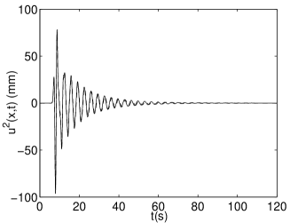
Figure 8: $2\pi$ times the spectrum (left panel) and time history (right panel) of the total displacement response to the cylindrical wave (radiated by a deep source located at $\mathbf{x^{s}}=(-65m,3000m)$) at the center of the summit segment of a single $40m\times 40m$ block. The dashed curves correspond to the semi-analytical (mode-matching, one mode) result and the solid curves to the numerical (finite-element) result.

Figure 8, depicts the spectrum and time history of the total displacement at the center of the summit segment of the block as computed by the mode-matching method (with account taken of one quasi-mode) and the finite-element method for a deep source. No noticeable differences are found between the results of the two methods of computation. The neglect of the quasi-modes of order larger than $0$ is valid for this block width. The block acts as a ribbon source of width $w$ located at the base segment.

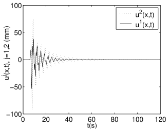
Figure 9: Comparison of $2\pi$ times the spectrum (top panels) and time history (bottom panels) of the total displacement on the ground in absence of block (solid curves) with the total displacement (dotted curves) at the center of the top segment (left panel) and at the center of the base segment (right panel) of a single $40m\times 40m$ block, for a deep source located at $\mathbf{x^{s}}=(-65m,3000m)$.

Figure 9 depicts the spectrum and the time history of the total displacement on the ground in the absence of the block as well as the total displacement at the centers of the top and base segments of the block for a deep source. In the time domain, a small increase of the duration, and a fairly-large increase of the peak amplitude, can be noticed, particularly on the top segment of the block, where the quasi displacement-free block mode makes itself felt. In the frequency domain, there is an increase of the maximum amplitude and the sharpness of the first resonance peak of the substructure at around $0.3Hz$, as noticed previously, to some extent, in [32, 10], and is a characteristic feature of the so-called soil-structure interaction. A similar phenomenon was mentioned in 6.3, and is due to the ability of shallow sources to excite Love modes in the configuration without blocks [21]. Here, a quasi-Love mode can be excited due to the presence of the block, which acts like a shallow (actually located on the ground) source. A similar fact was already noticed in [22], where the spectra of the displacement on the ground for a deep source (provoking only interference phenomena) was compared to that for a shallow source (provoking Love mode excitation).

The so-called soil-structure interaction consists (in the configuration with blocks) in a modification of the phenomenon from a state where interference (when a soft layer is present) or reflection (when the soft layer is absent) phenomena are dominant to a state where a quasi-Love mode is excited. This mode is excited because of the presence of the block in a configuration. In the absence of the latter, no mode can be excited.

Another point of view is that the block takes the form of an induced source at the top of the layer (see section 7.1), and it is now known that Love modes are excited when such a configuration is solicited by a line source near the boundaries of the layer [20].

A particular feature of the spectrum of the displacement when the block is present, (top-right subfigure of fig. 9) is that it vanishes at the base segment for $\displaystyle\nu_{00}^{DFB}\approx\frac{c_{2}}{2b}$, which is the fundamental displacement-free base block eigenfrequency. This is made evident in the field representation in the block and can be understood to be a geometrical effect which, in the case of a single block, corresponds to the excitation of a quasi-mode.

8.2 Results relative to one $50m\,\times\,30m$ block

The block is $50m$ high and $30m$ wide. The displacement-free base block eigenfrequencies are then $0.5$, $1.5Hz$, …..

Figure 10: Indications concerning the solution of the dispersion relation $\mathcal{F}=\mathcal{F}_{1}-\mathcal{F}_{2}=0$ for a single $50m\,\times\,30m$ block in a Mexico City-like site. In the left panel, the solid curve describes $\Re\left(\mathcal{F}_{1}\right)$ versus frequency ($\nu$ in Hz) and the dashed curve describes $\Re\left(\mathcal{F}_{2}\right)$ versus frequency. The right panel again contains two curves: the solid one describes $\Im\left(\mathcal{F}_{1}\right)$ versus frequency and the dashed curve describes $\Im\left(\mathcal{F}_{2}\right)$ versus frequency .

Figure 10 gives an indication of the modes of the configuration. One notes that the eigenfrequencies (frequencies at which $\Re(\mathcal{F}_{1})=\Re(\mathcal{F}_{2})$, at the least) are $\nu\approx 0.3\mbox{, }0.5\mbox{, }1.0\mbox{, }1.53\mbox{, }1.75\mbox{, }1.93$. The attenuations of the quasi-Love mode at $\nu\approx 0.3$ and $0.9$ Hz, and of the quasi displacement-free base block at $\nu\approx 0.5$ and $1.5Hz$ are relatively-small. As previously, the attenuation of the quasi stress-free base block (close to the zeros of $\tan\left(k^{2}b\right)$) at $\nu_{0,1}^{QSFB}\approx 1Hz$ is relatively-large.

In figs. 11 and 12, we plot the absolute values of the zeroth-order terms involved in the resolution of the linear system (115). The source terms $2\pi\|\cos(k^{2}b)P_{0}(\omega)/S(\omega)\|$ are once again close to the transfer functions calculated without the block for both locations of the source $\mathbf{x^{s}}=(0m,3000m)$ and $\mathbf{x^{s}}=(-3000m,100m)$.

The term $I_{0}^{(j)-}(k_{1},\omega)=\mbox{sinc}\left(k_{1}\frac{w}{2}\right)$ again has a small influence on $P_{0}(\omega)$. For a deep source, the main component of $P_{0}(\omega)$ comes from the integration over $\mathcal{I}_{1}$ (i.e. the solicitation of the block takes the form of interfering propagative waves traveling in the layer associated with bulk waves in the substratum) while for a shallow source, the main component of $P_{0}(\omega)$ comes from the integration over $\mathcal{I}_{2}$ (i.e. the solicitation of the block takes the form of propagative waves traveling in the layer associated with evanescent waves in the substratum, i.e., Love modes). The integral over $\mathcal{I}_{2}$ again dominates $Q_{00}(\omega)$.

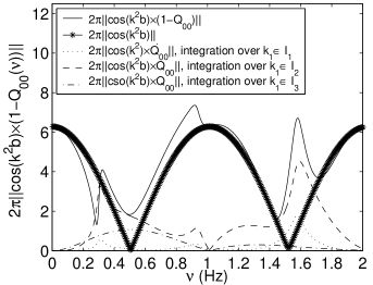
Figure 11: $2\pi\|E_{00}\|$.

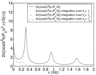
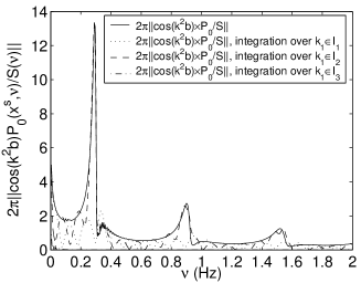
Figure 12: Driving agent $2\pi\|\cos(k^{2}b)P_{0}/S(\omega)\|$ for a deep source located at $\mathbf{x^{s}}=(0m,3000m)$ (left panel) and for a shallow source located at $\mathbf{x^{s}}=(-3000m,100m)$ (right panel).

8.2.1 Displacement field on the top and bottom segments of the block for deep line source solicitation

We now examine the displacement field on the horizontal boundaries of the block.

We first consider that the seismic disturbance is delivered to the site by a deep line source located at $\mathbf{x^{s}}=(0,3000m)$. This means that in absence of the block, the displacement field is mainly composed of propagative waves in the substratum and interfering propagative waves in the layer.

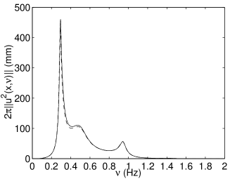
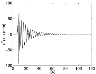
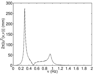
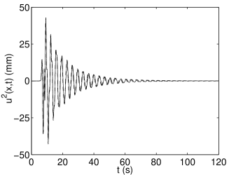
Figure 13: $2\pi$ times the spectra (left panels) and time histories (right panels) of the total displacement response to a cylindrical wave (radiated by a deep source located at $\mathbf{x^{s}}=(0m,3000m)$) at the center of the summit segment (top panels) and at the center of the base segment (bottom panels) of a single $50m\times 30m$ block. The dashed curves correspond to the semi-analytical (mode-matching, one mode) result, and the solid curves to the numerical (finite-element) result.

Figure 13, depicts the spectra and time histories of the total displacement at the center of the top and bottom segments of the block, as computed by the mode-matching method (with account taken of one quasi-mode) and the finite-element method, for a deep source. No noticeable differences are found between the results of the two methods of computation. The neglect of the quasi-modes of order larger than $0$ is valid for this block width. The block acts as a ribbon source of width $w$ located at the base segment.

Figure 14: Comparison of $2\pi$ times the spectrum (on the top) and time history (on the bottom) of the total displacement on the ground in absence of the block (solid curves) with the total displacement (dotted curves) at the center of the top segment (left panel) and at the center of the base segment (right panel) of a single $50m\times 30m$ block, for a deep source located at $\mathbf{x^{s}}=(0m,3000m)$.

Figure 14 depicts the spectra and the time histories of the total displacement on the ground in the absence of the block as well as the total displacement at the centers of the top and base segments of the block for a deep source. In the time domain, a small increase of the duration (although larger than in the $40m\times 40m$ block case), and a fairly-large increase of the peak amplitude, can be noticed, particularly on the top segment of the block, where the quasi displacement-free block mode makes itself felt.

In the frequency domain, there is an increase of the maximum amplitude and of the sharpness of the first resonance peak of the substructure, which is a characteristic feature of the soil-structure interaction. Again, the displacement field vanishes at the base segment for a frequency close to $\nu_{00}^{DF}$.

8.2.2 Displacement field on the top and bottom segments of the block for shallow line source solicitation

We now consider what happens when the seismic disturbance is delivered to the site by a shallow line source located at $\mathbf{x^{s}}=(-3000m,100m)$. This means that, in the absence of the block, the displacement field in the substructure is that of Love modes at the resonance frequencies of these modes.

Figure 15 compares the displacement on the ground in the absence of the block to that in the block (on the top and bottom segments thereof) for a shallow source. In the time domain, the durations are substantially the same when the block is present or absent, but the peak and cumulative amplitudes are larger in the presence of the block. In the frequency domain, both the sharpness and amplitude of the first peak, corresponding to the first Love mode in absence of the blocks, increase. This means that the soil-structure interaction obtained for a deep source is also found for a shallow source. The fact that the position of this peak is hardly shifted means that the structure of the quasi-Love mode is very nearly that of the Love mode existing in the absence of the block. However, the presence of the block enables this mode to be excited more efficiently than in its absence, i.e., when the site is solicited solely by the shallow source and not by waves re-emitted by the block.

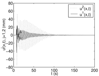
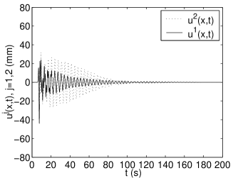
Figure 15: Comparison of $2\pi$ times the spectrum (on the top), and time history (on the bottom) of the total displacement on the ground in the absence of the block (solid curves) with the total displacement, (dotted curves) at the center of the top segment (left panel) and of the bottom segment (right panel) of a single $50m\times 30m$ block, for a shallow line source located at $\mathbf{x^{s}}=(-3000m,100m)$.

8.2.3 Displacement on the ground on one side of the block for deep line source solicitation

To obtain a more complete picture of the modification of the phenomena due to the presence of a block, we now focus our attention on the ground motion outside of the block.

The deep seismic line source is located at $\mathbf{x^{s}}=(0m,3000m)$.

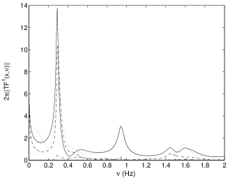
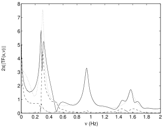
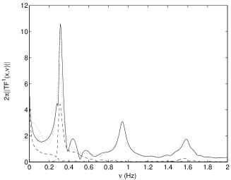
Figure 16: $2\pi$ times the transfer function (solid curves) of the total displacement on the ground at $\mathbf{x}=(20m,0m)$ (top-left), $\mathbf{x}=(30m,0m)$ (top-right), $\mathbf{x}=(150m,0m)$ (bottom-left), and $\mathbf{x}=(300m,0m)$ (bottom-right). The deep line source is located at $\mathbf{x^{s}}=(0m,3000m)$. The dotted curve represents the contribution along the interval $\mathcal{I}_{1}$, the dashed curve the contribution along the interval $\mathcal{I}_{2}$, and the dot-dashed curve the contribution along the interval $\mathcal{I}_{3}$.

Figures 16 represents $2\pi$ times the transfer function $u^{1}(\mathbf{x},\omega)/S(\omega)$ at various locations on the ground outside of the block, computed by the mode-matching method by taking into account only the zeroth-order quasi-mode. From the fact that the deep source is close to the vertical line passing through these ground locations, in the absence of the block, the first peak of the transfer function is principally due to the integral over $\mathcal{I}_{1}$ [21, 22]. The presence of the block induces: i) a double dependency of the first peak on the integrals over $\mathcal{I}_{1}$ and over $\mathcal{I}_{2}$ which leads to splitting of the first peak at some locations (as seen in the results at $\mathbf{x_{g}}=(150m,0m)$), ii) surface waves in the layer (represented by the contribution of the integration over $\mathcal{I}_{3}$) which normally are not excited in the case of a deep source, [21, 22]. The presence of the block allows the excitation of a quasi-Love mode as is testified by the importance of the integration over $\mathcal{I}_{2}$.

Fig. 17 shows once again that there is a good agreement between the results of the mode-matching method (with only the fundamental quasi-mode taken into account) and the finite element method.

Fig. 18 shows that when the block is present, the displacement field at a given location on the ground is somewhat different from what it is in absence of the block, even at a large (i.e. 300m) distance from the block, this being particularly evident in the response spectra. The duration and cumulative amplitude of the displacement fields have a tendency of increasing as one approaches the block, but not in monotonic manner, as manifested by what happens at $150m$.

This may be one of the causes of the spatial variability of the destructions noticed during the Michoacan earthquake. As shown by the form of the matrix in section 6.5, one can expect one building to have an effect on its neigbors via the waves traveling in the substructure and in particular in the layer and along the ground. Thus, the effect of one block on the other can vary in a way that depends on the distance of their separation. Nethertheless, the authors of [19] did not find substantial differences in response for varying building separations in the case of an idealized city composed of ten blocks. It may be that in order for this effect to be noticeable requires either a large distance of separation between blocks or a single block.

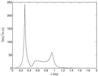
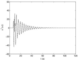
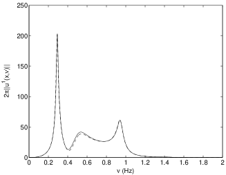
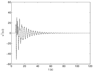
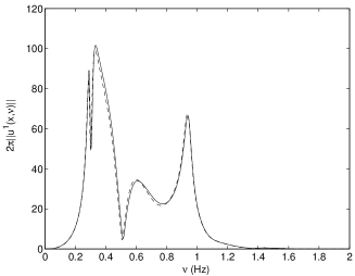
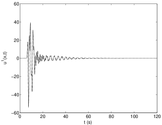
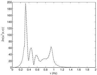
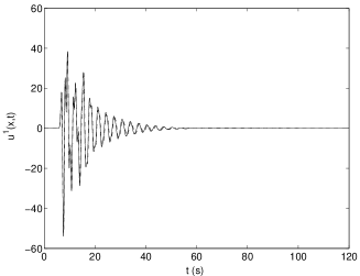
Figure 17: $2\pi$ times the spectrum (left panel) and time history (right panel) of the total displacement at various locations on the ground: (from the top to bottom) at 20m, 30m, 150, and 300m from the center of a single $50m\times 30m$ block. The dashed curves correspond to the semi-analytical (mode-matching) result (with only the fundamental quasi-mode taken into account), and the solid curves to the finite element result.

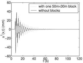
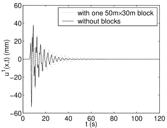
Figure 18: Comparison of $2\pi$ times the spectrum (left panel) and of the time history (right panel) of the total displacement on the ground in the absence of the block (solid curves) and in the presence of the block (dashed curves) at various locations on the ground: (from the top to the bottom) at 20m, 30m, 150, and 300m from the center of a single $50m\times 30m$ block. The deep line source is located at $\mathbf{x}^{s}=(0,3000m)$.

8.2.4 Displacement on the ground on one side of the block for shallow line source solicitation

When the seismic disturbance is delivered to the site by the wave radiated from a shallow line source located at $\mathbf{x^{s}}=(-3000m,100m)$, it should be recalled that, in the absence of the block, the first peak (associated with the first Love mode) is mainly composed of the component coming from the integration over $\mathcal{I}_{2}$, whereas we observe in fig. 19 that when the block is present, this peak is composed mainly of two components, one from integration over $\mathcal{I}_{1}$ and the other from integration over $\mathcal{I}_{2}$. However, this double dependence of the first peak finds no apparent translation in the time history of the displacement on the ground, as seen in fig. 20. In fact, we see in this figure that there are no substantial differences in the responses on the ground between the cases of the absence and presence of the block.

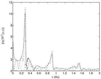
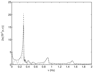
Figure 19: $2\pi$ times the transfer function, solid curve, of the total displacement on the ground at $\mathbf{x_{g}}=(150m,0m)$ (left panel), and $\mathbf{x_{g}}=(300m,0m)$ (right panel). The shallow source is located at $\mathbf{x^{s}}=(-3000m,100m)$. The dotted curve represents the contribution along the interval $\mathcal{I}_{1}$, the dashed curve represents the contribution along the interval $\mathcal{I}_{2}$, and the dotted-dashed curve represents the contribution along the interval $\mathcal{I}_{3}$.

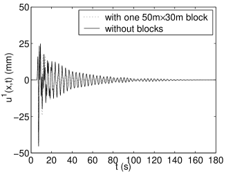
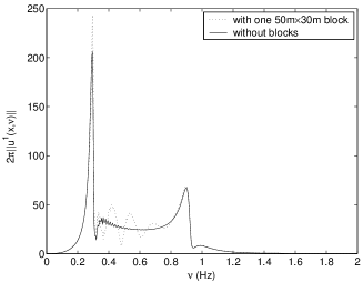
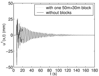
Figure 20: Comparison of $2\pi$ times the spectrum (left panel) and of the time history (right panel) of the total displacement on the ground in the absence of the block (solid curves) and in the presence of the block (dashed curves) at various locations on the ground: (from the top to the bottom) at 150 and 300m from the center of a single $50m\times 30m$ block. The shallow source is located at $\mathbf{x}^{s}=(-3000,100m)$.

8.2.5 Displacement in the substratum

The focus here is on the displacement field in the subtratum when the solicitation is due to a deep source located at $\mathbf{x}^{s}=(0,3000m)$.

As shown in fig. 21, the main components of the diffracted field (i.e. $u^{0}-u^{i}$) are those due to propagative and evanescent waves in the substratum, the latter being associated with a quasi-Love mode.

Figure 21: The solid curve represents $2\pi$ times the transfer function of the diffracted displacement at the interface between the substratum and the layer below the center of a single $50m\times 30m$ block. The dotted curve represents the contribution of the interval $\mathcal{I}_{1}$, the dashed curve the contribution of the interval $\mathcal{I}_{2}$ and the dot-dashed curve the contribution of the interval $\mathcal{I}_{3}$.

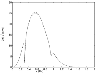
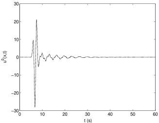
Figure 22: $2\pi$ times the spectrum (left panel) and time history (right panel) of the total displacement at the interface between the substratum and the layer below the center of a single $50m\times 30m$ block. The dashed curves result from the semi-analytical (mode-matching) computation, whereas the solid curves result from the numerical (finite element) computation . Note the splitting of the first peak.

The comparison of the results of the mode-matching and finite element methods is made in fig. 22. The time history of the total displacement field is mainly composed of the incident and specularly-reflected fields. Although a quasi-Love mode is excited, it hardly makes itself felt in the substratum.

9 Numerical results for two-block configurations in a Mexico City-like site

Let us now consider the configuration involving two blocks, which is the simplest configuration for studying inter-block coupling effects. The latter go by the name of structure-soil-structure interaction.

The two blocks, situated in a Mexico City-like environment, are located such that the center of the base segment of block 1 is (0m,0m) and that of block 2 is (-65m,0m).

The parameters of the site are: $\rho^{0}=2000$ kg/m³, $c^{0}$=600 m/s, $Q^{0}=\infty$, $\rho^{1}=1300$ kg/m³, $c^{1}$=60 m/s, $Q^{1}=30$, with the soft layer thickness being $h=50$ m. The material constants of the blocks are: $\rho^{2}=325$ kg/m³, $c^{2}$=100 m/s, $Q^{2}=100$.

The incident cylindrical wave is radiated by a deep line source located at (0m, 3000m).

Recall that the eigenfrequencies of the displacement-free base block are $\nu_{0m}^{FB}=\frac{c^{2}(2m+1)}{2b}$, and the Haskell frequencies are $\nu_{m}^{HASK}=\frac{2m+1}{2}\frac{c^{1}}{2h}$, wherein $m=0,1,2,...$. Thus, the Haskell frequencies are 0.3, 0.9, 1.5 Hz ,…

If the zeroth-order quasi-mode coefficient is relevant, the dispersion relation of the configuration takes the from:

$$\left(\mathcal{F}_{1}^{(1)}-\mathcal{F}_{2}^{(1)}\right)\left(\mathcal{F}_{1}^{(2)}-\mathcal{F}_{2}^{(2)}\right)-\mathcal{F}_{2}^{(12)}\mathcal{F}_{2}^{(21)}=\mathcal{F}=0$$ (138)

wherein $\mathcal{F}_{1}^{(j)}-\mathcal{F}_{2}^{(j)}=0$, $j=1,2$ is the dispersion relation of the configuration with one block of characteristics of the block $j$ (see eq.137) and the term $\mathcal{F}_{2}^{(12)}\mathcal{F}_{2}^{(21)}=\left(\cos\left(k^{2}b_{1}\right)Q_{00}^{(12)}\right)\left(\cos\left(k^{2}b_{2}\right)Q_{00}^{(21)}\right)$ accounts for the coupling between the two blocks.

9.1 Results relative to a two-block configuration consisting of a $50m\,\times\,30m$ block and a $40m\,\times\,40m$ block

Block 1 is $50m$ high and $30m$ wide and block 2 is $40m$ high and $40m$ wide. Their center-to-center separation is $65m$.

The displacement-free base block eigenfrequencies are: $\nu_{00}^{DFB}=0.5\mbox{, }1.5Hz...$ for block 1, and $\nu_{00}^{DFB}=0.625\mbox{, }1.875Hz...$ for block 2.

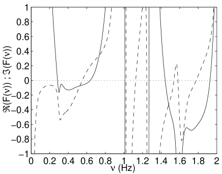
Figure 23: Indications concerning the dispersion relation for a system of two blocks, one with dimensions $50m\,\times\,30m$ and the other with dimensions $40m\,\times\,40m$. The solid curve represents $\Re(\mathcal{F})$ and the dashed curve $|\Im(\mathcal{F})|$.

Figure 23 gives an indication of the frequency of occurrence of the modes of the system. An eigenfrequency is a frequency for which $\Re\left(\mathcal{F}\right)=0$. The attenuation associated with a particular mode (at a frequency $\nu^{\star}$) is given by $\Im\left(\mathcal{F}(\nu^{\star})\right)$.

A quasi-Love mode is excited at $\nu\approx 0.3$. We could expect two different quasi displacement-free base block modes for a system with two non-identical blocks (at $\nu_{00}^{QDF}\approx 0.5$ and $0.625Hz$), but only one eigenfrequency, at $\approx 0.7Hz$, is found (actually this value is debatable, since the the eigenfrequency might actually correspond to a minimum of $\|\mathcal{F}\|$ rather than to a zero of $\mathcal{F}$). This means that: i) the modes of a complex configuration are not the union of the modes of the subsystems of which it is composed, ii) the single quasi displacement-free block mode results from the inter block coupling of the fields, i.e., the (structure-soil-structure interaction), iii) this mode is a coupled mode and is associated with a smaller attenuation than either of the corresponding modes of the two associated one-block configurations, iv) the correct expression of the modes of the system is the one given in section 6.5 involving the couplings between the blocks. In particular, the coupling matrix $Q_{00}^{(ij)}$, $i\neq j$ cannot be neglected.

To distinguish this mode from the quasi displacement-free base block mode for a single block that accounts only for the structure-soil interaction, we call it the multi-displacement-free base block mode.

9.1.1 Response on the top and bottom segments of the blocks

Now consider the response at the centers of the top segments of the two blocks.

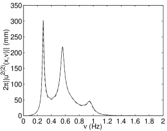
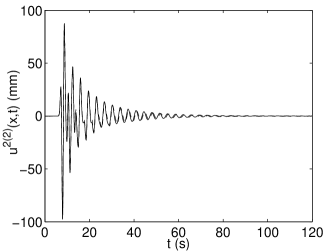
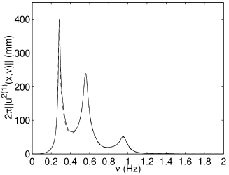
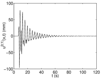
Figure 24: $2\pi$ times the spectrum (left panels) and time histories (right panels) of the total displacement of a configuration with two blocks for a deep seismic line source located at $\mathbf{x}^{s}=(0,3000m)$. The top panels apply to the field at the center of the top segment of block 2 ($40\times 40$ block). The lower panels apply to the field at the center of the top segment of block 1 ($50\times 30$ block). The dashed curves result from a computation via the semi-analytical (quasi-mode) method (taking account only of the zeroth-order quasi-mode in each block), whereas the solid curves result from a finite element computation.

The responses at these locations, as computed by the finite element and mode matching methods (with account taken only of the zeroth-order quasi-mode in each building), are seen in fig. 24 to be almost identical in each block. The peak at $\nu_{00}^{MDF}\approx 0.6Hz$, translates the excitation of the multi-displacement-free base block mode. This peak is sharper than the one encountered for only one block at $\nu_{00}^{QDF}$ (due to excitation of the quasi displacement-free base block mode), which fact is essentially due to its larger amplitude. The important sharpness of this peak is also related to the fact that the excited mode is a coupled mode. This suggests that the larger the number of blocks, the larger will be the response at the resonance frequency of the multi-displacement-free base block mode.

We compare in fig. 25 the results obtained in (at the centers of the top and bottom segments of) the two blocks with those on the ground (at the same locations as the centers of bottom segments of the blocks) in the absence of these blocks. In the time domain, a small increase of the duration and a more substantial increase of the peak and cumulative amplitudes can be observed, in particular on the top segments of the two blocks. These increases are more important than in the configurations with a single $40m\,\times\,40m$ or $50m\,\times\,30m$ block (see figs. 9 and 14), and is also somewhat more important in block 1 than in block 2, as already noticed in the cases of single blocks. The field vanishes at the center of the bottom segments at the displacement-free base frequencies: $\nu=0.5Hz$ for block 1 and $\nu=0.625Hz$ for block 2. This emphasizes the fact that the multi displacement-free block mode is different from the quasi displacement-free block mode of the configuration with only one block, and is a manifestation of geometrical features.

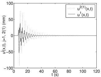
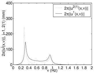
Figure 25: Comparison of $2\pi$ times the spectrum (left panels) and time history (right panels) of the total displacement on the ground in absence of blocks (solid curves) and in the presence of blocks (dashed curves). From the top to bottom: at the center of the summit segment of block $1$, at the center of the summit segment of block $2$, at the center of the base segment of block $1$, and at the center of the base segment of block $2$. The deep line source is located at $\mathbf{x}^{s}=(0,-3000m)$.

9.2 Results relative to a two-block configuration with two $40m\,\times\,40m$ blocks

The two blocks are $40m$ high and $40m$ wide and their center-to-center separation is 65m.

The displacement-free base block eigenfrequencies of the two blocks are 0.625, 1.875 Hz …

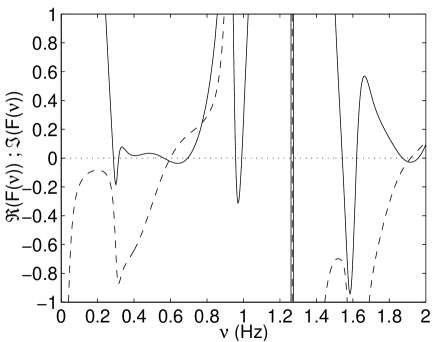
Figure 26: Indications concerning the dispersion relation for a configuration with two $40m\,\times\,40m$ blocks. The solid curve represents $\Re(\mathcal{F})$ and the dashed curve $\Im(\mathcal{F})$.

Fig. 26 gives an indication of the solutions of the dispersion relation $\mathcal{F}=0$. The eigenfreqencies corresponding to $\Re\mathcal{F}=0$, are seen to occur at $0.3$, $0.35$, $0.6$, $0.7$, $0.9$, $1.0$Hz… Some of them are close to each other and can be gathered together into the groups: $0.3-0.35$, $0.6-0.7$ and $0.9-1.0$ $Hz$. This suggests a splitting associated with the lifting of the degeneracy of eigenvalues. Nevertheless, the attenuations of the modes at $0.35$, $0.7$ and $0.9-1.0$ are very large, so that we can expect them to be hardly excited (as will be confirmed in the following results).

9.2.1 Response on the top and bottom segments of the blocks

In fig. 27 we see that the results obtained by the two computational methods pertaining to the response at the center of the summit segments of the two $40m\,\times\,40m$ blocks are nearly identical. The amplitude of the multi-displacement-free base block resonance peak is higher for two identical blocks, than it was for two different blocks. As pointed out during the previous discussion of the dispersion relation of the configuration, no splitting of the first and second peaks is noticed because of the high attenuation of one of each pair of split modes. On the contrary, the large response due to the excitation of the other one of the pairs of split modes is due to the small attenuation of these modes. Notice also that the second (quasi displacement-free base mode) peaks in the spectra of the figure are larger than the first peaks, in contrast to what was obtained for two dissimilar blocks.

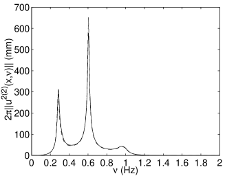
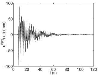
Figure 27: $2\pi$ times the spectra (left panel) and time histories (right panel) of the total displacement at the center of the summit segment of block 2 (top panels), and at the center of the summit segment of block 1 (bottom panels), as computed by the mode-matching method (accounting only for the zeroth-order quasi-mode) (dashed curves) and by the finite element method (solid curves) for a configuration with two $40m\,\times\,40m$ blocks solicited by the cylindrical wave radiated by a deep line source.

In fig. 28 we compare the displacement in the two blocks (in particular, at the centers of the summit and base segments) with the displacement on the ground in the absence of these blocks. The response of the two blocks are, in fact, identical, due to the deep source being located on the vertical dividing line between the two blocks. One observes an increase of the duration and of the peak and cumulative amplitudes that is larger than for two different blocks, in particular, on the top segments. This increase seems to be due to the much more stronger response associated with the excitation of the multi displacement-free base mode block. This hypothesis is backed up by the fact that the said mode is more weakly excited on the base segment and at the same time the time history is much closer to that of the configuration with no blocks. Finally, the displacement at the center of the base segments vanishes at the frequency of occurrence of the displacement-free base mode of the block (which is not a mode of the global configuration) and is slightly different from the corresponding multi-displacement-free block mode eigenfrequency.

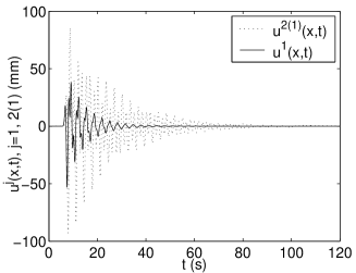
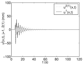
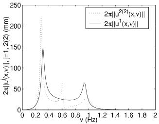
Figure 28: Comparison of $2\pi$ times the spectrum (left panels) and of the time history (right panels) of the total displacement on the ground in the absence of blocks (solid curves) and in the presence of the blocks (dashed curves). From the top to the bottom: at the center of the summit segment of block $1$, at the center of the summit segment of block $2$, at the center of the base segment of block $1$, and at the center of the base segment of block $2$. Two $40m\,\times\,40m$ blocks solicited by the cylindrical wave radiated by a deep line source located at $\mathbf{x}^{s}=(0,-3000m)$.

9.3 Results relative to a two-block configuration with two $50m\,\times\,30m$ blocks

The blocks are $50m$ high and $30m$ wide and their center-to-center separation is $65m$.

The displacement-free base block eigenfrequencies are $0.5$, $1.5Hz$, …..

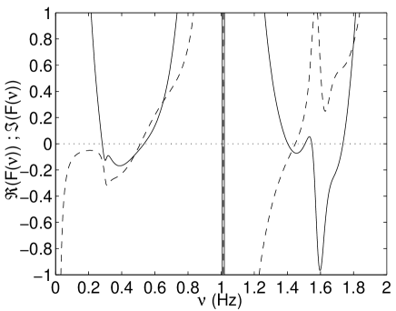
Figure 29: Indications concerning the dispersion relation $\mathcal{F}=0$. The solid curves represent $\Re(\mathcal{F})$ and the dashed curves $\Im(\mathcal{F})$.

Fig. 29 gives an indication of the solution of the dispersion relation. Eigenfreqencies (i.e., solutions of $\Re\mathcal{F}=0$) are found at $0.3$, $0.55$, $1.0$, $1.4$… The attenuations associated with the quasi-Love mode at $0.3Hz$ and the multi displacement-free base block mode at $0.55Hz$ are rather small. The eigenfrequencies are not close to each other, contrary to the case of two identical $40m\,\times 40m$ blocks.

9.3.1 Response on the top and bottom segments of the blocks

The response at the centers of the summit segments of both blocks computed by the finite element method is compared in fig. 30 to the corresponding response computed by the mode matching method (with account taken only of the zeroth-order quasi-mode. Once again, we observe these responses to be almost identical. Moreover, the amplitude of the multi- displacement-free base block resonance peak is observed (in the same figure) to be higher for two identical blocks, than it was for two different blocks.

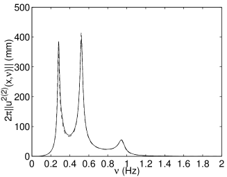
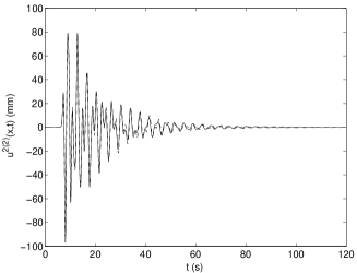
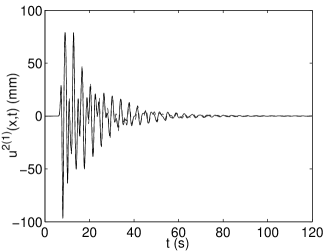
Figure 30: $2\pi$ times the spectra (left panel) and time histories (right panel) of the total displacement at the center of the summit segment of block 2 (top panels), and of the block 1 (bottom panels), as computed by the mode-matching method (with account taken only of the zeroth-order quasi-mode (dashed curves) and the finite element method (solid curves).

In fig. 31 we compare the displacements in the two blocks (i.e., at the centers of the summit and base segments) with the displacement on the ground (at the same points as occupied by the centers of the base segments of the blocks) in the absence of the blocks. The response of the two blocks are identical for the previously-mentioned reasons. A much larger increase of the duration and of the peak and cumulative amplitudes (particularly on the top segments) is obtained for the two identical blocks than for two different blocks. This increase seems to be due to the much stronger response at the frequency corresponding to the excitation of the multi displacement-free base block mode. Once again, the displacement at the center of the base segments vanishes at a frequency corresponding to the occurrence of the displacement-free base mode of the block.

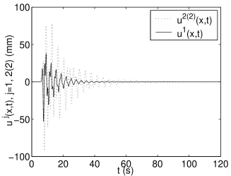
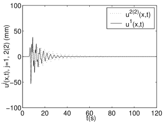
Figure 31: Comparison of $2\pi$ times the spectrum (left panels) and of the time history (right panels) of the total displacement on the ground in the absence of blocks (solid curves) and in the presence of blocks (dashed curves). From the top to the bottom: at the center of the summit segment of block $1$, at the center of the summit segment of block $2$, at the center of the base segment of block $1$, and at the center of the base segment of block $2$. Two $50m\,\times\,30m$ blocks solicited by the cylindrical wave radiated by a deep line source located at $\mathbf{x}^{s}=(0,-3000m)$.

9.3.2 Response on the ground

In order to get another grip on the phenomena that are produced when two blocks are present, we now focus on the displacement field at points on the ground outside of the blocks.

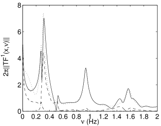
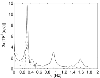
Figure 32: $2\pi$ times the transfer function (solid curve) of the total displacement on the ground at $\mathbf{x_{g}}=(150m,0m)$ (left panel), and $\mathbf{x_{g}}=(300m,0m)$ (right panel) for a two $50m\,\times\,30m$ block configuration solicited by the cylindrical wave radiated by a deep line source located at $\mathbf{x^{s}}=(0m,3000m)$. The dotted curve represents the contribution along the interval $\mathcal{I}_{1}$, the dashed curve the contribution along the interval $\mathcal{I}_{2}$, and the dotted-dashed curve the contribution along the interval $\mathcal{I}_{3}$.

Fig. 32 depicts $2\pi$ times the transfer function $u^{1}(\mathbf{x},\omega)/S(\omega)$ resulting from a computation by the mode-matching method. The influence of two blocks on the contribution of the various types of waves traveling in the layer is close to the one we noticed when only one block is present (see fig. 16). The amplitude of the first peak is more important than that of the one in fig. 16.

The comparison in fig. 33 between the displacement in the presence of the blocks and in their absence shows a small increase of the amplitude and of the duration in the time domain, this depending non-linearly on the location on the ground. In the frequency domain, the amplitude of the first peak is larger than for a single block.

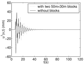
Figure 33: Comparison of $2\pi$ times the spectrum (left panels) and of the time history (right panels) of the total displacement on the ground at $\mathbf{x_{g}}=(150m,0m)$ (top panels), and $\mathbf{x_{g}}=(300m,0m)$ (bottom panels) in the absence of blocks (solid curves) and in the presence of the blocks (dashed curves). Case of two $50m\,\times\,30m$ blocks solicited by the cylindrical wave radiated by a deep line source located at $\mathbf{x}^{s}=(0,-3000m)$

10 Snapshots of the displacement fields for one- and two-block configurations in a Mexico City-like site

In order to better visualize the excitation of the quasi-Love mode due to the presence of one or two blocks in a Mexico City-like site, we show, in figs. 34 and 35, the snapshots at various instants, of the displacement field, for one $50m\,\times\,30m$ block, and two identical $50m\,\times\,30m$ blocks, respectively, in response to the cylindrical wave radiated by a deep line source located at $\mathbf{x}^{s}=(0m,3000m)$.

$t=12s$

$t=18s$

$t=24s$

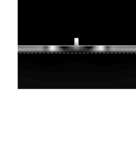
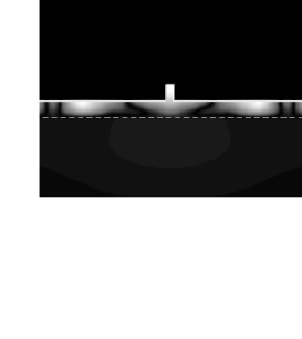
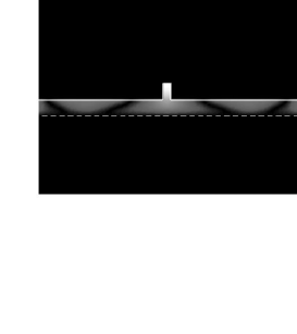
$t=30s$

$t=36s$

$t=42s$

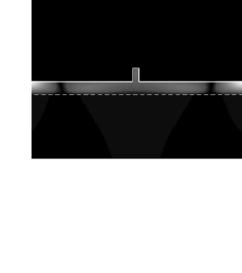
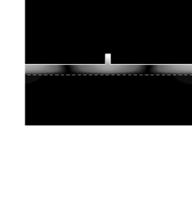
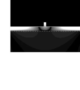
Figure 34: Snapshots at various instants, $t=12s$, $t=18s$, $t=24s$, $t=30s$, $t=36s$, $t=42s$, of the total displacement field for one $50m\,\times 30m$-block configuration, solicited by the cylindrical wave radiated by a deep line source located at $\mathbf{x}^{s}$=(0m,3000m).

$t=21s$

$t=42s$

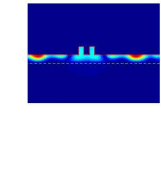
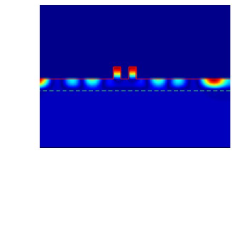
Figure 35: Snapshots at $t=21s$ and $t=42s$ of the total displacement field for two identical $50m\,\times 30m$- block configuration, solicited by the cylindrical wave radiated by a deep line source located at $\mathbf{x}^{s}$=(0m,3000m).

We notice, in the layer regions of these figures, waves that are re-radiated from the base segments of the blocks and which evolve into a field with a series of nodes and anti-nodes characteristic of a sum of modes dominated by the quasi-Love modes. Coupling between the two blocks (structure-soil-structure iteraction) is also noticeable in fig. 35 at $t=21s$.

11 Conclusions and preview of the contents of the companion paper

The response, to the cylindrical wave radiated by a line source located in the substratum, of a finite set of non-equally sized, non-equally spaced blocks, each block modeling one, or a group of buildings, in welded contact with a soft layer overlying a hard half space, was investigated in a theoretical manner via the mode matching technique.

The capacity of this technique to account for the complex phenomena provoked by the presence of blocks on the ground was demonstrated by comparison of the numerical results to which it leads to those obtained by a finite element method.

It was shown that the presence of blocks induces a modification of the phenomena that are produced by the configuration without blocks, or of a configuration of closed blocks disconnected from the geophysical half-space. In particular, the blocks modify the dispersion relation of what, in the absence of the blocks, constitutes the Love modes.

Three different and complementary points of view were developed (in the framework of the mode matching theory) concerning the dispersion relation relative to the configuration with blocks. The first emphasizes the role of the substructure (i.e. the geophysical (flat ground/layer/substratum) structure ). The second emphasizes the role of each particular block of the superstructure. The third point of view emphasizes the couplings of the fields in the superstructure with those in the substructure.

The first two points of views enable the definition of two new types of modes relative to the configuration with blocks: the quasi-Love modes, which are small perturbations of the Love mode (which can exist when no blocks are present), and the quasi displacement- free base block modes, which are small perturbations of the displacement- free base block mode (which can exist when no geophysical structure is present).

These two types of quasi-modes account for coupling between a particular block of the superstructure with the substructure, but not for the couplings between blocks (when more than one block is present). Thus, the so-called soil-structure interaction is shown to be due to the excitation of quasi Love modes.

The third point of view emphasizes the coupling between blocks (when more than one block is present). It was shown that this coupling, manifested by the existence of coupling matrices in the expressions for the quasi mode amplitudes, is of the same form as the coupling between one particular block and the substructure, which underlines the fact that the coupling between blocks is carried out via the substructure.

The study of the dispersion relation for the multi-block configurations is very complex, but can be carried numerically. This was done for a two-block configuration and showed that a multi displacement-free base block mode can be produced. The latter was shown to correspond to a coupled mode, constituted by a combination of quasi displacement-free base block modes of each block, which are no longer excited as such in a configuration with more than one block. The multi displacement-free base block mode was shown to account for the so-called structure-soil-structure interaction.

It was underlined that the modes of a complete one- or multi-block configuration do not constitute the reunion of the modes of the individual component structures. Thus, the phenomena for a complete $N$ block configuration are not the sum of the phenomena for $N-1,N-2,..,0$ block configurations.

The excitation of these modes was then studied in the particular case of one and two blocks. A common feature of the influence of one/or more blocks is the excitation of the quasi-Love mode, which occurs even for solicitation by the waves radiated by a deep source (recall that, for this type of solicitation, it is not possible to excite ordinary Love modes in a flat ground (i.e., no blocks)/soft horizontal layer/hard substratum configuration [21]). The trace of quasi-Love mode excitation in the frequency domain was shown to be: i) for a deep source, a shift to lower frequency and an increase of the amplitude of the first (lowest-frequency) peak of the response, and ii) for a shallow source (the case in which waves whose structure is close to that of Love waves already exist in the layer and substratum in the absence of the block(s)), an increase of the amplitude, and little or no shift, of the first resonance peak.

As concerns deep sources, the change of the phenomena, from a configuration without blocks (for which there exist only bulk waves in the geophysical structure), to one with blocks (for which there exist quasi-Love modes characterized by a field in the substratum that is predominantly a surface wave in the substratum) is a manifestation of the so-called soil-structure interaction.

Quasi displacement-free base block modes are encountered only for configurations with one block whereas multi displacement-free base block modes are excited in configurations with two (and presumably, more) blocks. Both of these modes are excited with incident waves that are radiated either from deep or shallow sources. The multi displacement-free base block mode is more energetic and corresponds to a coupled mode. Its excitation is tied up with the so-called structure-soil-structure interaction.

The modifications of frequency-domain response (and less so for the time-domain response) were found to be fairly substantial, even when only one block is present, at large distances from the block on the ground.

Generally speaking, the peak and cumulative amplitudes and duration of the time histories are larger for a one- and two-block configuration than for flat ground, especially at locations within the block, but no spectacular effects, such as those noticed during the Michoacan earthquake were found in the numerical simulations, either for the one- or two-block ”cities”.

A configuration involving a larger number of blocks is difficult to study theoretically in the framework of the mode-matching formulation, which is why configurations with an infinite number of blocks, each one of which is close to the average shape and composition of the blocks of typical cities, is investigated in the companion paper. It is also shown in this paper that, beyond of the order of ten identical blocks, the response of the laterally-finite city is very close to that of the city with an infinite number of blocks. More importantly, it is found in the companion paper, that the phenomena are quite different, for configurations with a large number of identical blocks, from those for a small number of identical or non-identical blocks, and that the said phenomena for a large number of blocks are evocative of those observed during earthquakes in urban areas such as Mexico City.

This indicates that it is probably not sufficient to carry out experiments and numerical simulations on an isolated building [35, 23, 45] in order to predict correctly the seismic response of the building when it is surrounded by other buildings (the situation of most buildings in a typical city).

Appendix A An auxiliary problem: fields in the layer and in the substratum when the seismic distrubance takes the form of a ribbon source of width $w$ located in the layer

The problem is to determine the total fields $u^{1}(\mathbf{x},\omega)$ and $u^{0}(\mathbf{x},\omega)$, when the configuration without blocks (i.e. involving only a soft layer and a hard half space) is solicited by a horizontal ribbon source of width $w$ centered at $\mathbf{x}^{s}$ in the soft layer.

A.1 Boundary conditions and field representations

The fields satisfy the continuity of displacement and traction conditions on $\Gamma_{h}$, i.e., (23) and (24), the vanishing traction condition on $\Gamma_{g}$ (19), and the outgoing wave (radiation) condition.

In the layer and in the substratum the field representations are:

$$u^{1}(\mathbf{x},\omega)=u^{1i}(\mathbf{x},\omega)+\int_{-\infty}^{\infty}\left(A^{1}(k_{1},\omega)e^{-\mbox{i}k_{2}^{1}x_{2}}+B^{1}(k_{1},\omega)e^{\mbox{i}k_{2}^{1}x_{2}}\right)e^{\mbox{i}k_{1}x_{1}}\frac{dk_{1}}{k_{2}^{1}}~{},$$ (139)

and

$$u^{0}(\mathbf{x},\omega)=\int_{-\infty}^{\infty}B^{0}(k_{1},\omega)e^{\mbox{i}\left(k_{1}x_{1}+k_{2}^{0}x_{2}\right)}\frac{dk_{1}}{k_{2}^{0}}~{},$$ (140)

respectively.

A.2 The (incident) field radiated by a ribbon source of width $w$

By employing the Green’s theorem, the incident field can be written as:

$$u^{i1}(\mathbf{x},\omega)=\int_{\mathbb{R}^{2}}G(\|\mathbf{x}-\mathbf{y}\|,\omega)s^{i1}(\mathbf{y},\omega)d\varpi(\mathbf{y})\mbox{; }\forall\mathbf{x},\in\mathbb{R}^{2}~{},$$ (141)

wherein $\mathbf{y}$ is a vector from the origin $O$ and pointing to a generic point in the sagittal plane $(y_{1},y_{2})$, $G(\|\mathbf{x}-\mathbf{y}\|,\omega)$ the 2D free-space Green’s function, and $s^{i1}(\mathbf{y},\omega)$ the source density function:

$$s^{i1}(\mathbf{y},\omega)=\frac{S(\omega)}{w}\left[H\left(y_{1}-x_{1}^{s}+\frac{w}{2}\right)-H\left(y_{1}-x_{1}^{s}-\frac{w}{2}\right)\right]\delta\left(y_{2}-x_{2}^{s}\right)~{},$$ (142)

wherein $H(~{}.~{})$ is the Heaviside function and $\delta(~{}.~{})$ the Dirac delta distribution.

Introducing (142) into (141), enables the incident field to be written as:

$$u^{i1}(\mathbf{x},\omega)=\frac{\mbox{i}}{4\pi}\int_{\infty}^{\infty}S(\omega)e^{\mbox{i}\left(k_{1}(x_{1}-x_{1}^{s})+k_{1}^{1}|x_{2}-x_{2}^{s}|\right)}\mbox{sinc}\left(k_{1}\frac{w}{2}\right)\frac{dk_{1}}{k_{2}^{1}}~{},$$ (143)

wherein sinc$(\zeta):=\frac{\sin\zeta}{\zeta}$.

A.3 Expression of the fields in the the presence of a ribbon source of width w

The introduction of the field representations (139) and (140) into the boundary conditions (with the appropriate projection), leads, after the resolution of the resulting linear system, to:

• for $x_{2}\geqq x_{2}^{s}$:

  $$u^{1}(\mathbf{x},\omega)=\frac{\mbox{i}S(\omega)\mu^{1}}{2\pi\mu^{0}}\int_{-\infty}^{\infty}\frac{\cos\left(k_{2}^{1}\left(x_{2}^{s}-h\right)\right)+\mbox{i}\frac{\mu^{0}k_{2}^{0}}{\mu^{1}k_{2}^{1}}\sin\left(k_{2}^{1}\left(x_{2}^{s}-h\right)\right)}{\cos\left(k_{2}^{1}h\right)-\mbox{i}\frac{\mu^{1}k_{2}^{1}}{\mu^{0}k_{2}^{0}}\sin\left(k_{2}^{1}h\right)}\times\\ \cos\left(k_{2}^{1}x_{2}\right)e^{\mbox{i}k_{1}(x_{1}-x_{1}^{s})}\mbox{sinc}\left(k_{1}\frac{w}{2}\right)\frac{dk_{1}}{k_{2}^{0}}~{},$$ (144)

• for $x_{2}\leqq x_{2}^{s}$:

  $$u^{1}(\mathbf{x},\omega)=\frac{\mbox{i}S(\omega)\mu^{1}}{2\pi\mu^{0}}\int_{-\infty}^{\infty}\frac{\cos\left(k_{2}^{1}\left(x_{2}-h\right)\right)+\mbox{i}\frac{\mu^{0}k_{2}^{0}}{\mu^{1}k_{2}^{1}}\sin\left(k_{2}^{1}\left(x_{2}-h\right)\right)}{\cos\left(k_{2}^{1}h\right)-\mbox{i}\frac{\mu^{1}k_{2}^{1}}{\mu^{0}k_{2}^{0}}\sin\left(k_{2}^{1}h\right)}\\ \cos\left(k_{2}^{1}x_{2}^{s}\right)e^{\mbox{i}k_{1}(x_{1}-x_{1}^{s})}\mbox{sinc}\left(k_{1}\frac{w}{2}\right)\frac{dk_{1}}{k_{2}^{0}}~{},$$ (145)

and

$$u^{0}(\mathbf{x},\omega)=\frac{\mbox{i}S(\omega)\mu^{1}}{2\pi\mu^{0}}\int_{-\infty}^{\infty}\frac{e^{\mbox{i}(k_{1}(x_{1}-x_{1}^{s})+k_{2}^{0}(x_{2}-h))}}{\cos\left(k_{2}^{1}h\right)-\mbox{i}\frac{\mu^{1}k_{2}^{1}}{\mu^{0}k_{2}^{0}}\sin\left(k_{2}^{1}h\right)}\mbox{sinc}\left(k_{1}\frac{w}{2}\right)\cos\left(k_{2}^{1}x_{2}^{s}\right)\frac{dk_{1}}{k_{2}^{0}}~{}.$$ (146)

References

- [1] Aki K. & Larner K.L., 1970, Surface motion of a layered medium having an irregular interface due to incident plane SH waves, J.Geophys.Res., 75, 933-954.
- [2] Bard P.Y. & Wirgin A., 1996, Effects of buildings on the duration and amplitude of ground motion in mexico city, Bull.Seism.Soc.Am., 86, 914-920.
- [3] Bécache E., Joly P. & Tsogka C., 2001, Fictitious domains, mixed finite elements and perfectly matched layers for 2D elastic wave propagation, 9, 1175-1203, J.Comput.Acoust..
- [4] Boutin C. & Roussillon P., 2004, Assessement of the urbanisation effect on seismic response, Bull.Seism.Soc.Am., 94, 252-268.
- [5] Boutin C. & Roussillon P., 2006, Wave propagation in presence of oscillators on the free surface, Int.J.Engrg.Sci., 44, 180-204.
- [6] Cardenas-Soto M. & Chavez-Garcia F.J., 2003, Regional path effect on seismic wave propagation in central Mexico, Bull.Seism.Soc.Am., 93, 973-985.
- [7] Cardenas-Soto M. & Chavez-Garcia F.J., 2006, Seismic wavefield analysis in Mexico City using accelerometric arrays, Abstracts of the First European Conference on Earthquake Engineering and Seismology, SSS, Geneva, 166.
- [8] Chavez-Garcia F.J. & Bard P.Y., 1994, Site effects in Mexico-city height years after the september 1985 Michoacan earthquakes, SoilDyn.&Earthq.Engrg., 13, 229-247.
- [9] Chavez-Garcia F.J. & Salazar L., 2002, Strong motion in central Mexico: a model on data analysis and simpler modeling, Bull.Seism.Soc.Am., 92, 3087-3101.
- [10] Clouteau D. & Aubry D., 2001, Modification of the ground motion in dense urban areas, J.Comput.Acoust., 9, 1-17.
- [11] Collino F. & Tsogka C., 2001, Application of the PML absorbing layer model to the linear elastodynamic problem in anisotropic heterogeneous media, 66, 294-305, Geophys.
- [12] Doby R., Idriss I.M. & Ng E., 1979, A reply, Bull.Seism.Soc.Am., 69, 2127-2128.
- [13] Faeh D., Suhadolc P., Mueller St. & Panza, G.F., 1994, A Hybrid method for the estimation of ground motion in sedimentary bains: quantitative modeling for Mexico City, Bull.Seism.Soc.Am., 84, 1711-1797.
- [14] Fernandez-Ares A. & Bielak J., 1973, Urban seismology: interaction between earthquake ground motion and multiple buildings in urban regions, in ESG 2006, Bard P.-Y., Chaljub E., Cornu C., Cotton F. & Guéguen P. (eds.), LCPC, Paris, 87-96.
- [15] Flores J., Novaro O. & Seligman T.H., 1987, Possible resonance effect in the distribution of earthquake damage in Mexico City, Nature, 326.
- [16] Furumura T. & Kennett B.L.N., 1998, On the nature of regional seismic phase-III. The influence of crustal heterogénéity on the wavefield for subduction earthquakes: the 1989 Michoacan, and 1995 Copala, Guerro, Mexico earthquake, Geophys.J.Intl., 135, 1060-1085.
- [17] Groby J.P., 2005, Modélisation de la propagation des ondes élastiques générées par un séisme proche ou éloigné à l’intérieur d’une ville, PhD Thesis, Université de la Méditerranée-Aix-Marseille II.
- [18] Groby J.P. & Tsogka C., 2006, A time domain method for modeling viscoacoustic wave propagation, J.Comput.Acoust., 14, 201-236.
- [19] Groby J.P., Tsogka C. & Wirgin A., 2005, Simulation of seismic response in a city-like environment, Soil Dyn.&Earthq.Engrg., 25, 487-504
- [20] Groby J.-P. & Wirgin A., 2004, On the causes of anomalous seismic response in an urban site with a two-component soft layer overlying a hard substratum, EGU 1st General Assembly, Nice.
- [21] Groby J.P. & Wirgin A., 2005, 2D ground motion at a soft viscoelastic layer/hard substratum site in response to SH cylindrical sesimic waves radiated by deep and shallow line sources I. Theory, Geophys.J.Intl., 163, 165-191.
- [22] Groby J.P. & Wirgin A., 2005, 2D ground motion at a soft viscoelastic layer/hard substratum site in response to SH cylindrical sesimic waves radiated by deep and shallow line sources II. Numerical results, Geophys.J.Intl., 163, 192-224.
- [23] Guéguen P., 2000, Interaction sismique entre le sol et le bâti: de l’interaction sol-structure à l’interaction site-ville, Phd thesis, Université Grenoble I, Grenoble.
- [24] Guéguen P., Bard, P.Y. & Chávez-Garcia F.J., 2002, Site-City seismic interaction in Mexico city-like environments: an analytical study, Bull.Seism.Soc.Am., 92, 794-811.
- [25] Haghshenas E., Jafari M., Bard P.-Y., Moradi A.S. & Hatzfeld D., 2006, Preliminary results of site effects assessment in the city of Tabriz (Iran) using earthquakes recording, in ESG 2006, Bard P.-Y., Chaljub E., Cornu C., Cotton F. & Guéguen P. (eds.), LCPC, Paris, 993-1001.
- [26] Hill N.R. & Levander A.R., 1984, Resonances of low-velocity layers with lateral variations, Bull.Seism.Soc.Am., 74, 521-537.
- [27] Iwata T., Kagawa T. Petukhin A. & Onishi Y., 2006, Basin and crustal structure model for strong ground motion simulation in Kinki, Japan, in ESG 2006, Bard P.-Y., Chaljub E., Cornu C., Cotton F. & Guéguen P. (eds.), LCPC, Paris, 435-442.
- [28] Jennings P.C., 1970, Distant motions from a building vibration test, Bull.Seism.Soc.Am., 60, 2037-2043.
- [29] Jennings P.C. & Bielak J., 1973, Dynamics of building-soil interaction, Bull.Seism.Soc.Am., 63, 9-48.
- [30] Kjartansson E., 1979, Constant Q wave propagation and attenuation, J.Geophys.Res., 84,4737-4748.
- [31] Levander A.R & Hill N.R., 1984, P-SV resonances in irregular low-velocity surface layer, Bull.Seism.Soc.Am., 75, 847-864.
- [32] Lombaert G., Clouteau D., Ishizawa O. & Mezher N., 2004, The city-site effect : a fuzzy substructure approach and numerical simulations, In Doolin et al. ed., Proc. 11th Intl.Conf. on Soil Dyn.&Earthq.Engrg., vol2, 68-74.
- [33] Luco J.E. & Contesse L., 1993, Dynamic structure-soil-structure interaction, Bull.Seism.Soc.Am., 62, 449-462.
- [34] Maeda N., Nakajima Y., Matsuda I. & Abeki N., 2006, Evaluation of seismic amplification characteristics at a university campus with complicated relief of basement, in ESG 2006, Bard P.-Y., Chaljub E., Cornu C., Cotton F. & Guéguen P. (eds.), LCPC, Paris, 443-451.
- [35] Manos G.C., Demosthenous M., Triamataki M., Yasin B. and Skalkos P., 1995, Construction and instrumentation of a 5 storey masonry infilled RC building at the Volvi-Thessaloniki Euro-Seistest site: correlation of measured and numerically predicted dynamic properties, in Proceedings of the Third International Conference on Earthquake Engineering, Amman, Jordan, 2, 449-462.
- [36] Mateos J.L., Flores J., Novaro O., Seilgman T.H. & Alvarez-Costado J.M., 1993, Resonant response models for the valleys of Mexico - II The trapping of horizontal P waves, Geophys.J.Intl.,113, 449-462.
- [37] Morse P.M. & Feshbach H., 1953, Methods of Theoretical Physics, Mc Graw-Hill, New York, 1953.
- [38] Perez-Rocha L.E., Sanchez-Sesma F.J. & Reinoso E., 1991, Three-Dimensional site effects in mexico-city: evidence from the accelerometric network observation and theorical results, In Proc. 4th Intl. Conf. on Seismics Zonation, volume II, 327-334.
- [39] Rial J.A., 1989, Seismic wave resonances in 3-D sedimentary basins, Geophys.J.Int., 99, 81-90.
- [40] Roussillon P., 2006, Interaction sol-structure et interaction site-ville: aspects fondamentaux et modélisation, Phd thesis, INSA, Lyon.
- [41] Savage B.K., 2004, Regional Seismic wavefield propagation, PhD Thesis, California Institute of Technology.
- [42] Semblat J.-F., Duval A.-M. & Dangla P., 2000, Numerical analysis of seismic wave amplification in Nice (France) comparison with experiments, Soil Dyn.&Earthq.Engrg., 19, 347-362.
- [43] Semblat J.F., Guégen P., Kham M., Bard P.Y. & Duval A.M., 2003, Site-city interaction at local and global scales, In Proc. 12th European Conf. on Earthq.Engrg., paper no. 807.
- [44] Shaw D.E., 1979, Comment on ”Duration characteristics of horizontal components of strong-motion earthqauke records”, Bull.Seism.Soc.Am., 69, 2125-2126.
- [45] Todorovska M.I., 2002, Full-scale experimental studies of soil-structure interaction, ISET J.Earthqu.Tech., 39, 139-165.
- [46] Trifunac M.D., 1972, Interaction of a shear wall with the soil for incident plane SH wave, Bull.Seism.Soc.Am., 62, 63-83.
- [47] Tsogka C. & Wirgin A., 2003, Simulation of seismic response in an idealized city, Soil Dynam.Earthquake Engrg., 23, 391-402.
- [48] Wirgin A. & Groby J.P., 2006, Amplification and increased duration of earthquake motion on uneven stress-free ground, https://hal.ccsd.cnrs.fr/ccsd-00076746, http://fr.arxiv.org/abs/physics/0605239.
- [49] Wirgin A. & Groby J.-P., 2006, Amplification and increased duration of earthquake motion on uneven stress-free ground, in ESG 2006, Bard P.-Y., Chaljub E., Cornu C., Cotton F. & Guéguen P. (eds.), LCPC, Paris, 559-568.
- [50] Wong H.L. & Trifunac M.D., 1974, Surface motion of sediment-elliptical alluvial valley for incident plane SH waves, Bull.Seism.Soc.Am., 64, 1389-1408.