The Social Network of Contemporary Popular Musicians

Abstract

In this paper we analyze two social network datasets of contemporary musicians constructed from allmusic.com (AMG), a music and artists’ information database: one is the collaboration network in which two musicians are connected if they have performed in or produced an album together, and the other is the similarity network in which they are connected if they where musically similar according to music experts. We find that, while both networks exhibit typical features of social networks such as high transitivity, several key network features, such as degree as well as betweenness distributions suggest fundamental differences in music collaborations and music similarity networks are created.

I Introduction

Developments in computer and information technologies have allowed users to search for information they need on the Internet, rather than in the traditional arena of libraries or printed media. Particularly, developments in e-commerce technology have produced large commercial retailers of thousand of products serving millions of customers each day. E-comerce technology has reduced the cost of inventory storage and distribution, leading to what is known as the long-tail phenomenon and04 . This is related to the distribution of sales of a general item (books, CDs, DVDs, etc.), which generally decays with a power law distribution —a few items are sold in high volumes while most items suffer low sales volume. Therefore, by reducing the storage and distribution costs, it can be profitable for companies to concentrate on selling those less popular items, whose total amount can then overcome the incomes of a best-seller. Several websites, such as Amazon [http://www.amazon.com], allow on-line users to access any product by navigating through a network of links between items. Besides the commercial impact of allowing low-sales items to gain visibility, this kind of networks are sources of information about product similarity, category structures, and so forth.

In this paper, we analyze the topology of two social networks of contemporary popular musicians taken from the AllMusic database of music metadata [http://www.allmusic.com]. The content on the database is created by professional data entry staff, editors and writers. We work with two datasets, that of the collaboration network and the similarity network of artists in the database. The networks were constructed as follows: two artists were connected in the collaboration network when they have worked on one or more albums together, while they were connected in the similarity network by music experts of AllMusic according to some criteria.

There are several reasons that make these networks interesting. First, studying the collaboration network, formed naturally by the actual professional acts of artists, may teach us how musical tendencies spread via formation of profession relationships between musicians, which could prove worthwhile for musicology. Second, studying the similarity network, which is a large-scale result of human experts’ perception of music, may help in inventing recommendation systems in which machines are trained to perform the same task, and eventually help users discover music easier ell02 .

We will see, both networks show typical characteristics of real-world networks such as high transitivity and the small-world property, as some other have shown lim03 ; gle03 ; can06 . However, the discrepancies of the two sets, notably in the degrees and the betweenness centralities of same vertices, suggest a fundamental difference between the two networks.

II The Datasets

On a typical artist’s page on the allmusic.com database, we can find hyperlinks to other artists under various categories: “Similar Artists”, “Worked With”, “Followers”, etc. We can regard the existence of a link between two artists as having a tie in a social network. Using links in the category “Similar Artists” that had been created by the music experts of allmusic.com, we constructed the similarity network. Here, Mick Jagger of the Rolling Stones is connected to Tina Turner or David Bowie. On the other hand, using links in another category “Worked With”, we constructed the collaboration network, where Mick Jagger is now connected to other members of the Rolling Stones, such as Keith Richards or Charlie Watts, and others .

The similarity network is composed of $32,377$ vertices (artists) and $117,621$ edges, and the collaboration network is composed of $34,724$ vertices and $123,082$ edges. These two networks have $8,509$ vertices in common. These common vertices have $24,950$ edges in the similarity network, and $20,232$ edges for the collaboration network, between themselves. We can visualize this as Fig. 1. The two subnetworks defined on these common vertices will enable us to conduct a direct comparison study between similarity and collaboration link patterns.

Figure 1: The structure of the data sets studied in this paper. Two sets of network data have an intersection consisting of common vertices. These common vertices and the edges between them (similarity or collaboration) comprise the subnetworks.

III Basic Network Properties

In this section, we study several key properties of the networks, such as the degree distribution, transitivity, nearest-neighbor degree correlation, component structure and the Freeman centrality of vertices. They are summarized in Table 1 and Fig. 2.

	Similarity network		Collaboration network
	entire	intersection	entire	intersection
$n$	32 377	8 509	34 724	8 509
$m$	117 621	24 950	123 122	20 232
size of $S_{0}$	30 384 (94$\%$)	7 219 (85$\%$)	30 945 (89$\%$)	6 054 (71$\%$)
$\bar{d}~{}(d_{\mathrm{max}})$	6.5 (22)	6.0 (20)	6.4 (23)	6.3 (19)
$C$	0.185 ($18.5\%$)	0.178 ($17.8\%$)	0.182 ($18.2\%$)	0.171 ($17.1\%$)
	$131$	$55$	$508$	$143$
$k_{\mathrm{max}}$	R.E.M.	Eric Clapton	P. Da Costa	P. Da Costa
				R. Van Gelder
highest-betweenness	Sting	Sting	P. Da Costa	P. Da Costa
artist

Table 1: Summary of several network characteristics of similarity, collaboration, and intersection subnetworks: number of vertices $n$, number of edges $m$, number of vertices in the largest component $S_{0}$ and its percentage among all vertices, mean geodesic path $\bar{d}$ in $S_{0}$, diameter $d_{max}$ of $S_{0}$, global clustering coefficient $C$, the highest-degree $k_{\max{max}}$ and the corresponding artist(s), and the artist with the highest betweenness.

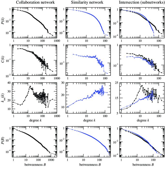
Figure 2: The cumulative degree distribution $P(k)$ (first row), the local clustering coefficient $C(k)$ (second row), the nearest–neighbor degree distribution $k_{nn}$ (third row), and the cumulative betweenness centrality distribution $P(B)$ for the collaboration (circle) and similarity (diamond) networks.

III.1 Mean geodesic length, diameter and component structure

A prominent feature of a complex network is the called the “small-world effect” str98 which means that the shortest paths (also called geodesics) between vertices is very small compared to the system size. The longest geodesic in the network is called its diameter. We see in Table 1 that average geodesic length $\bar{d}$ is smaller than $7$, while the diameter is no larger than $23$ in each network.

A component of a network is the set of vertices that are connected via one or more geodesics, and disconnected (i.e., no geodesics) from all other vertices. Typically, networks possess one large component that contains a majority of vertices. In Table 1 we see that with the exception of the collaboration subnetwork, each giant component contains $\sim 90\%$ of the vertices.

III.2 Degree distribution

The number of vertices linked to a vertex is called its degree, usually denoted $k$. The degree distribution $p_{k}$ is the fraction of vertices in the system with degree $k$. Many real-world networks, including the Internet and the worldwide web (WWW), are known to show a right-skewed distribution, often a power law $p_{k}\propto k^{-\tau}$ with $2<\tau<3$. More frequently, the cumulative degree distribution $P(k)=\sum_{k^{\prime}=k}^{\infty}p_{k^{\prime}}$, the fraction of vertices having degree $k$ or larger, is plotted. A cumulative plot avoids fluctuations at the tail of the distribution and facilitates the evaluation of the power coefficient $\tau$ in case the network follows a power law.

We see in Figure 2 that collaboration network exhibit power-law degree distributions near their tails, $p(k)\sim k^{-3}$, following a straight line in a log-log representation. We obtain a similar result when looking at its intersection subnetwork.

On the other hand, the similarity network closely follows an exponential form of $p_{k}\sim\exp{-0.12k}$, while its intersection subnetwork follows $p_{k}\sim\exp{-0.15k}$. As such, there is a huge difference $k_{\mathrm{max}}$: artist R.E.M. and Eric Clapton are the most connected in the entire dataset and the subnetwork with degrees $131$ and $55$ respective, while in the collaboration dataset, Paulinho Da Costa tops in both cases with degrees $508$ and $143$ (tied with the legendary recording engineer Rudy Van Gelder of the famed Blue Note label), several times larger than his counterparts in the similarity network.

III.3 Transitivity

Transitivity, or clustering, is an indication of how cliquish (tightly knit) a network is. It is quantified by the abundance of triangles in a network, where a triangle is formed when three vertices are all linked to one another. It can be quantified by the global clustering coefficient $C$, defined as

$$C=\frac{3\times\textrm{number of triangles}}{\textrm{number of connected triples}}.$$ (1)

Here, a connected triple means a pair of vertices connected via another vertex. Since a triangle contains three triples, $C$ is equal to the probability that two neighbors of a vertex is connected as well. Typical social networks have $C$ of fractions of percent, and in Table 1 that the music networks show values of $17\%$–$18\%$. The reason that this indicates an abundance of triangles is that in the most random graph model of comparable size ($n$ and $m$), $C$ is almost negligible — for example, with $n=34\,724$ and $m=123\,082$, a random graph has $C=0.02\%$.

A closely related yet distinct measure is the local clustering coefficient $C_{i}$ of each vertex $i$ (defined for the case $k_{i}>1$) defined as

$$C_{i}=\frac{\textrm{number of connected pairs of neighbors of $i$}}{\textrm{number of pairs of neighbors of $i$}=\frac{1}{2}k_{i}(k_{i}-1)},$$ (2)

which is the fraction of pairs of neighbors of a vertex are connected.

Often the local clustering is plotted as a function of degree $k$ defined as the average of $C_{i}$ over all vertices with a given degree $k$:

$$C(k)=\langle C_{i}\rangle\bigl{|}_{k_{i}=k}.$$ (3)

Some real-world networks are known to show a behavior of $C(k)\propto k^{-1}$, usually attributed to the hierarchical nature of networks rav02 . In Fig. 2 we have plotted the local $C(k)$. We observe that $C(k)$ decreases as $k^{-1}$ for range $30\lesssim k\lesssim 300$ for the collaboration network, but the decreasing pattern is not as clear for other data sets.

III.4 Degree correlations

We have also calculated the average nearest-neighbor degree $k^{\mathrm{nn}}$ as a function of $k$,

$$k^{\mathrm{nn}}(k)=\sum_{k^{\prime}=0}^{\infty}k^{\prime}p(k^{\prime}|k),$$ (4)

where $p(k^{\prime}|k)$ is the fraction of edges that are attached to a vertex of degree $k$ whose other ends are attached to vertex of degree $k^{\prime}$. Thus $k^{\mathrm{nn}}$ is the mean degree of the vertex we find by following a link emanating from a vertex of degree $k$.

The $k^{\mathrm{nn}}$ for our four datasets are plotted in Fig. 2 (third row). Here we see another difference between the two main networks [apart from that observed in $P(k)$]. While for the similarity network it is a nearly monotonic, increasing function, for the collaboration network it is not at all a simple form. The evolution of $k_{nn}(k)$ is related with the assortativity of the network new02 , which indicates the tendency of a vertex of degree $k$ to associate with a vertex of the same $k$. When $k_{nn}(k)$ is an increasing function of $k$, which is the case of the similarity network (see Fig. 2, third row, central plot), the network is assortative. In other words, the most connected artists are prone to be similar to other top connected artists. On the other hand, we can observe that the collaboration network is rather noisy (Fig. 2, third row, first plot). The first section of the $k_{nn}(k)$, for values up to 12 is assortative while the tail is not. The assortativeness for small values of $k$ could relate with band size in which all components obviously collaborate with all the others. The same reasoning does not apply for larger values. It could also be argued the assortativity observed in the similarity network is not a consequence of collaboration between artists.

A closely-related concept is the degree-degree correlation coefficient $r$, which is the Pearson correlation coefficient for degrees of vertices at either end of a link:

$$r = \frac{\sum_{i}k_{i}^{2}k_{i}^{\mathrm{nn}}-(2m)^{-1}\bigl{[}\sum_{i}k_{i}^{2}\bigr{]}^{2}}{\sum_{i}k_{i}^{3}-(2m)^{-1}\bigl{[}\sum_{i}k_{i}^{2}\bigr{]}^{2}}\simeq\frac{\sum_{k}k^{2}k^{\mathrm{nn}}(k)p_{k}-z^{-1}\bigl{[}\sum_{k}k^{2}p_{k}\bigr{]}^{2}}{\sum_{k}k^{3}p_{k}-z^{-1}\bigl{[}\sum_{k}k^{2}p_{k}\bigr{]}^{2}},$$ (5)

where $p_{k}$ is the degree distribution, $\sum_{i}$ denotes sum over vertices and $\sum_{k}$ denotes sum over degrees. We can clearly see the connection between $r$ and $k^{\mathrm{nn}}(k)$. In the case of a monotonically increasing (decreasing) $k^{\mathrm{nn}}(k)$ which means, as mentioned before, that high-degree vertices are connected to other high-degree (low-degree) vertices and vice versa, it results in a positive value of $r$, as in the case of the similarity network which has $r=0.184$ (for the intersection portion of the network, $r=0.188$). In other cases, however, we cannot read it off easily: for the entire collaboration network, $r=-0.00575$ while for its intersection portion $r=0.0372$. The collaborative networks result, especially, is an interesting observation, since most social networks are known to show positive degree-degree correlation (as seen in the similarity network), and it is thought to be originating in part from the community structure new03 .

III.5 The betweenness (Freeman) centrality

Given the inhomogeneity of link patterns around vertices in a complex network, we could certainly imagine that the position and roles of vertices will vary significantly from one vertex to another. Centrality, as its name suggests, is a concept that differentiates vertices according to how influential, or central, they are in a network. Degree is one kind of centrality, since it would be reasonable to assume that people with particularly many acquaintances can be looked as being important figures. However, degree is primarily local in scope (and talking loudly does not mean you are affecting others more effectively than somebody who speaks quietly but very eloquently, so to speak), and to overcome its shortcomings social scientists have in particular developed various measures of centrality. For our networks’ dataset we choose to study the betweenness or Freeman centrality fre77 .

The idea behind this centrality measure is that a central vertex will act as a relay of information between vertices, a role endowed thanks to being on a geodesic between vertices (hence the name betweenness). Considering a vertex has a relay of information so that it has a “power to withhold information …or to refuse to pass on requests for information” seems intuitively appropriate for communication networks systems, and recently has been studied on the Internet as well goh02 ; vaz02 .

The reason for choosing this centrality to study these networks was that we were interested in gaining a glimpse of how musical influences (considered as information) might spread via the complex network of artists. Especially, “crossover” musicians are becoming more common these days, and we were anticipating that those people who produce albums across genres were important in musical developments of the multiple genres, and by becoming bridges between genres, might have higher betweenness centrality.

The definition of Freeman (betweenness) centrality $B_{l}$ of a vertex $l$ is defined as

$$B_{l}=\frac{1}{2}\sum_{i,j}\frac{g_{ilj}}{g_{ij}},$$ (6)

where $g_{ij}$ is the total number of geodesics between vertices $i$ and $j$, and $g_{ilj}$ is the number of the ones that pass through the vertex $l$.

In Fig. 2 (fourth row) we have plotted the cumulative fraction $P_{B}(k)$ of Freeman centralities for our datasets. We see that this distribution is highly skewed for both cases (with no differences at the subnetworks). Similar results were obtained by different authors goh02 ; vaz02 in other kind of networks. In Table 1 there is list of artists with the highest betweenness centrality in each data set. It is interesting to note that in the cases of similarity network data, the highest-degree vertex is not the highest-centrality vertex. We will discuss this point deeply in the next section.

IV Comparison of self-organized network and artificial network

An interesting question, as we have posed in the beginning of this paper, is how differently an individual is represented in different types of networks. People belong to many spheres of social activity, and their relationship with the same people may well be different in each sphere. In fact, the two of our intersection data set seem to be quite different. Among the $24,950$ and $20,232$ edges belonging to the collaboration and similarity data respectively, there are only $464$ common edges, so having worked together does not necessarily (practically not at all) translate into being classified as musically similar.

To see how different the individuals’ roles are in these two networks, in Table 2 we have indicated the top ten high betweenness scorers from either network, along with their ranks in the other data set. The difference is evident. For example, Paulinho Da Costa, the prolific Brazilian percussionist, ranked first in the collaboration network, is ranked at merely $2,933^{\mathrm{th}}$ in the similarity network. On the other hand, Sting, ranked at the top in the similarity network, is ranked at $1,406^{\mathrm{th}}$ in the collaboration network. In fact, none of the top ten artists in either network is ranked as high in the other network. Quantitatively, the Spearman correlation of the two ranks is $0.255$, indicating that the two are only slightly correlated.

COLLABORATION
Rank	Artist	rank in	comments
		similarity network
1	Paulinho Da Costa	2,933	Percussionist
2	Jim Keltner	5,468	Percussionist
3	Ron Carter	2,689	Bassist
4	Rudy Van Gelder	5,468	Recording engineer
5	Dean Parks	5,468	Guitarist
6	Herbie Hancock	299	Jazz pianist
7	Randy Brecker	4,073	trumpetist and flugenhornist
8	Jim Horn	4,517	Saxophonist
9	Dann Huff	3,620	Guitarist
10	Tony Levin	1,471	Bassist
SIMILARITY
Rank	Artist	rank in	comments
		collaboration network
1	Sting	1,406	singer, bassist
2	Joni Mitchell	837	singer, song writer
3	Eric Clapton	23	guitarist, singer
4	Quincy Jones	46	producer, trumpeter
5	Gil Evans	396	jazz pianist
6	Jimi Hendrix	3,047	guitarist, singer
7	M. Davis1/C. Parker2	41	trumpeter1, saxophonist2
8	Aretha Franklin	67	singer
9	Lenny Kravitz	2,446	singer, songwriter
10	Jeff Beck	463	guitarist

Table 2: The ten top-ranked artists in betweenness in either of the intersection dataset, with their ranks in the other data set indicated. The two ranks are moderately correlated with Spearman coefficient $0.255$.

If we look at Table 2 in more detail, we can see each vertex’s characteristics and/or specialty in action. Artists with the largest betweenness in the collaboration data set are primarily instrumentalists (except for Rudy Van Gelder, a prolific recording engineer of the famed Blue Note and Verve labels, among many), and indeed all nine musicians are most famous for their virtuosity in the indicated instruments. They must have been invited to work in a multitude of recording sessions for various projects (in our data set, Paulinho da Costa has had $143$ collaborators in the intersection data set, and $508$ overall in the entire data set of collaborations), possibly bridging musicians of different styles to result in a high betweenness. However that did not necessarily translate into their perceived musical styles becoming as varied. A possible explanation for that is that some musicians adapt to the style of music that the recording artists requires.

Considering the similarity network, it is remarkable to find an exponential decay in their degree distribution, since many social networks exhibit a power law new03 . Nevertheless we must be very cautious since the similarity network has been designed by human perception (the opinion of experts). In this way, the evaluation of how similarity (i.e. musical tendencies) spreads will always be filtered by a subjective opinion, a fact that may cover (and filter) the real structure of the similarity network. In this sense, efforts have been made during the last years in order to obtain numerical algorithms to evaluate, in a rigorous and objective way, similarity between songs (and artists) ell02 . Nevertheless, how to capture music similarity as perceived by humans is still an open field.

V Conclusions

In this paper, we have looked at various network properties of two types of music networks. One was the collaboration relations among musicians which must have evolved naturally, and the other was the musical similarity amongst them, which was entirely constructed via human perception of music. We have analyzed the structural properties of the networks, observing that both networks share small world properties together with a clustering coefficient following a power law. The latter indicates the existence of a certain modularity that depends on the vertex degree (leading to a hierarchy). In this way, better connected artists form larger clusters than those of artists with less connections. Despite networks are constructed with artists as vertices and a certain connection between them (similarity/collaboration), we obtain different results, such as the degree distribution, which follows a power law in the collaboration network and has exponential decay in the similarity network. In addition, the Freeman centrality shows that vertices with highest betweenness are completely different at both networks, a fact that indicates that collaboration is not the mechanism for similarity spreading. Reciprocally, playing similar music is not an ingredient to predict collaboration links. It is indeed usual that artists collaborate with artists from a complete different style. The difference between the similarity and collaboration networks rules out the possibility of using collaboration data to infer music similarity. This would have proved convenient because collaboration data is easier to gather and definitely more objective.

References

- (1) Anderson, C. (2004) “The long tail”, Wired, 12.10 October 2004.
- (2) Cano, P., Celma, O., Koppenberger, M. and Buldú, J.M., (2006) “Topology of music recommendation networks”, Chaos 16, 013107.
- (3) Ellis, D.P., Withman, B., Berenzweig, A. and Lawrence, S., (2002) “The quest of ground truth in musical artist similarity”, Proc. Int. Symposium on Music Information Retrieval, 170–177 (2002), Paris.
- (4) Freeman, L., (1997) “A set of measures of centrality based upon betweenness”, Sociometry, 40, 35–41.
- (5) Gleiser, P. and Danon, L., (2003) “Community structure in Jazz”, Advances in Complex Systems 6, 565–573 (2003).
- (6) Goh, K.-I., Oh, E., Jeong, H., Kahng, B. and Kim, D., (2002) “Classification of scale-free networks”, Proc. Natl. acad. Sci. USA, 99, 12583–12588.
- (7) Goh, K.-I., Oh, E., Kahng, B. and Kim, D., (2003) “Betweenness centrality correlation in social networks”, Phys. Rev. E, 67, 017101.
- (8) de Lima e Silva, D., Medeiros Soares, M., Henriques, M.V.C., Schivani Alves, M.T., de Aguilar, S.G., de Carvalho, T.P., Corso, G. and Lucena, L.S., (2003) “The complex network of the Brazilian popular music”, Physica A, 332, 559–565.
- (9) Newman, M.E.J., (2002) “Assortative Mixing in Networks”, Phys. Rev. Lett., 89, 208701.
- (10) Newman, M.E.J., (2002) “The structure and function of complex networks”, SIAM Review, 45, 167–256.
- (11) Ravasz, E., Somera, A.L., Mongru, D.A., Oltvai, Z.N. and Barab si, A.-L., (2002) “Hierarchical Organization of Modularity in Metabolic Networks”, Science, 30, 1551–1555.
- (12) Watts, D.J. and Strogatz, S.H.,(1998) “Collective dynamics of small-world networks”, Nature, 393, 440–442.
- (13) Vázquez, A., Pastor-Satorras, R. and Vespignani., A., (2002) “Large-scale topological and dynamical properties of the Internet”, Phys. Rev. E, 65, 66130.