Cascades of Dynamical Transitions in an Adaptive Population

Abstract

In an adaptive population which models financial markets and distributed control, we consider how the dynamics depends on the diversity of the agents’ initial preferences of strategies. When the diversity decreases, more agents tend to adapt their strategies together. This change in the environment results in dynamical transitions from vanishing to non-vanishing step sizes. When the diversity decreases further, we find a cascade of dynamical transitions for the different signal dimensions, supported by good agreement between simulations and theory. Besides, the signal of the largest step size at the steady state is likely to be the initial signal.

I Introduction

Many natural and artificial systems consist of a population of agents with coupled dynamics. Through their mutual adaptation, they are able to exhibit interesting collective behavior. Although the individuals are competing to maximize their own payoffs, the system is able to self-organize itself to globally efficient states. Examples can be found in economic markets and communication networks Anderson1988 ; Challet1997 ; Wei1995 ; Schweitzer2002 .

An important factor affecting the behavior of an adaptive population is the dependence of the payoffs on the environment experienced by the individual agents. The payoffs facilitate the agents to assess the preferences of their decisions, hence inducing them to take certain actions when they experience similar dynamical environment in the future. Thus, the payoff function is crucial to the mechanism of adaptation.

As a prototype of an adaptive population, the Minority Game (MG) considers the dynamics of the buyers and sellers in a model of the financial market, in which the minority group is the winning one Challet1997 . A good indicator of the mutual adaptation of the agents is the reduction of the variance of the buyer population to values below those of random fluctuations Challet1997 . Furthermore, this variance has a universal dependence on the complexity of the strategies adopted by the agents, dropping to a minimum when the complexity is reduced to a universal critical value, and rapidly rising thereafter Savit1999 ; Manuca2000 . Theoretical studies using the replica method Challet2000 ; Marsili2000 and the generating functional Heimel2001 ; Coolen2005 confirmed these general trends.

The agents in the original version of MG uses a step payoff function Challet1997 ; Savit1999 ; Manuca2000 , meaning that the payoffs received by the winning group are the same, irrespective of the winning margin (the difference between the majority and minority group). Latter versions of MG uses a linear payoff function Challet2000 ; Marsili2000 ; Heimel2001 ; Coolen2005 , in which the payoffs increase with the winning margin. Other payoff functions yield the same macroscopic behavior in their dependence of the population variance on the complexity of strategies Li2000 ; Lee2003 . Thus, the behavior of the population is universal as long as the payoff function favors the minority group. A recent extension of the MG considers payoff functions which reward the minority agents only when they win by a large margin, but punish them when the winning margin is small de Martino2004 . The extended model displays a smooth crossover from a minority game to a majority game when the payoff function is tuned.

However, when one considers details beyond the population variance, one can find that the agents self-organize in different ways induced by different payoff functions. For a payoff function that favors a large winning margin, the distribution of the buyer population is doubled-peaked Challet1997 . This shows that the dynamics of the population self-organizes to favor large winning margins of either the buyers or sellers, since the agents have adapted themselves to maximize their payoffs.

In this paper, we compare the behavior of MGs using step and linear payoffs. Previously, we found that the population variance scales as a power law of the diversity for a step payoff Wong2004 ; Wong2005 . Diversity refers to the variance of the initial biases of the strategy payoffs of the agents. In a population with diverse preferences of strategies, the adaptation rate is slow, resulting in small fluctuations of the buyer or seller population. As we shall see, when the payoff function becomes linear, the scaling relation between the variance and the diversity for the step payoff is replaced by a continuous dynamical transition from a vanishing variance at high diversity to a finite variance at low diversity. The dynamical transition is due to the payoffs being enhanced by large winning margins at low diversity. Furthermore, for systems with multi-dimensional signals feeding the strategies, the dynamical transition in each dimension do not take place at the same transition point. Rather, there is a cascade of dynamical transitions for the different signal dimensions. This rich behavior demonstrates the flexibility of an adaptive population for self-organizing to states in which agents maximize their payoffs, and is hence important in the modeling of economics and distributed control.

II The Minority Game

The Minority Game model consists a population of N agents competing for limited resources, N being odd Challet1997 . Each agent makes a decision 1 or 0 at each time step, and the minority group wins. For economic markets, the decisions 1 and 0 correspond to buying and selling respectively, so that the buyers can win by belonging to the minority group, which pushes the price down, and vice versa. For typical control tasks such as the distribution of shared resources, the decisions 1 and 0 may represent two alternative resources, so that less agents utilizing a resource implies more abundance. The decisions of each agent are responses to the environment of the game, described by signal $\mu^{*}(t)$ at time t, where $\mu^{*}(t)=1,...,D$. These responses are prescribed by strategies, which are binary functions mapping the D signals to decisions 1 or 0. In this paper, we consider endogenous signals, which are the history of the winning bits in the most recent m steps. Thus, the strategies have an input dimension of $D=2^{m}$, and the parameter $\alpha\equiv\textit{D}/N$ is referred to as the complexity. Before the game starts, each agent randomly picks s strategies. Out of her s strategies, each agent makes decisions according to the most successful one at each step. The success of a strategy is measured by its cumulative payoff, as explained below.

Let $\xi_{i}^{\mu}(t)=\pm 1$ when the decisions of strategy a are 1 or 0 respectively, responding to signal $\mu$. Let $a^{*}(i,t)$ be the strategy adopted by agent i at time t. Then $A(t)\equiv\sum_{i}\xi_{a^{*}(i,t)}^{\mu^{*}(t)}/N$ is the excess demand of the game at time t. The payoff received by strategy $a$ is then $-\xi_{a}^{\mu^{*}(t)}\varphi(\sqrt{N}A(t))$, where $\varphi$ is the payoff function. For step and linear payoffs, $\varphi(\chi)=\mathrm{sgn}\chi$ and $\chi$ respectively. (Here, we have implicitly assumed that an agent does not consider the impact of adopting a strategy, although the excess demand is only dependent on the adopted ones.) Let $\Omega_{a}(t)$ be the cumulative payoff of strategy a at time t. Then its updating dynamics is described by

$$\Omega_{a}(t+1)=\Omega_{a}(t)-\xi_{a}^{\mu^{*}(t)}\varphi(\sqrt{N}A(t)).$$ (1)

Diversity of initial preferences of strategies is introduced by adding random biases $\omega_{ia}$ to the cumulative payoffs of strategy a (a$=2,...,s$) of agent i with respect to her first one. The biases are drawn from a Gaussian or binomial distribution with mean 0 and variance R. The ratio $\rho\equiv\textit{R}/N$ is referred to as the diversity.

To monitor the mutual adaptive behavior of the population, we measure the variance $\sigma^{2}/N$ of the population making decision 1, defined by

$$\frac{\sigma^{2}}{N}\equiv\frac{N}{4}\langle[A^{\mu^{*}(t)}(t)-\langle\mathrm{A}^{\mu^{*}(t)}(t)\rangle]^{2}\rangle$$ (2)

where the average is taken over time when the system reaches the steady state, and over the random distribution of strategies and biases.

III Dynamical Transitions

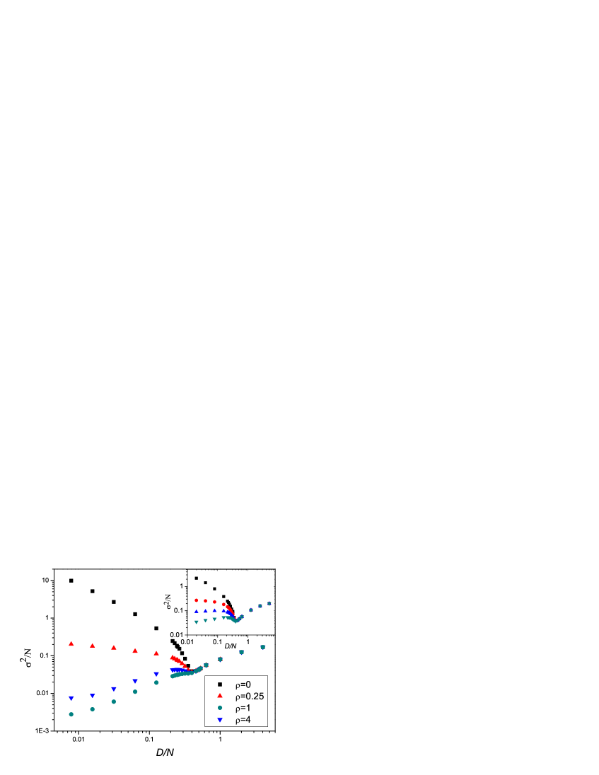
Figure 1: $\sigma^{2}/N$ versus $\alpha$ with linear payoffs, for $\rho$=0, 0.25, 1, 4, respectively, $N$=251, $s$=2, 1000 samples. Inset: The corresponding plot for step payoffs.

As shown in Fig. 1, the dependence of the variance $\sigma^{2}/N$ on the complexity $\alpha$ for linear payoffs is very similar to that for step payoffs Wong2004 ; Wong2005 . For $\alpha$ above a universal critical value $\alpha_{c}(\approx 0.3)$, the variance drops when $\alpha$ is reduced. The effects of introducing the diversity is also similar to that for step payoffs, namely, the variance remains unaffected when $\alpha>\alpha_{c}$, but decreases significantly with the diversity when $\alpha<\alpha_{c}$.

However, there are differences when one goes beyond this general trend. As shown in Fig. 2, the variance curves at different values of $\alpha$ cross at at $\rho=\rho_{c}\approx 0.16$, indicating the existence of a continuous phase transition at $\rho_{c}$ from a phase of vanishing variance at large $\rho$ to a phase of finite variance at small $\rho$.

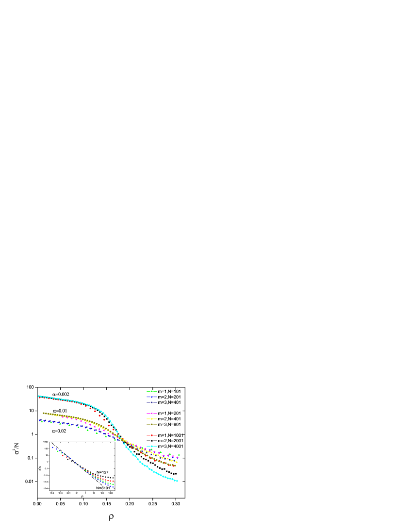
Figure 2: $\sigma^{2}/N$ versus $\rho$ with linear payoffs, $\alpha=0.002,0.01,0.02$ for different $m$ and $N$; Inset: $\sigma^{2}/N$ versus $\rho$ with step payoffs with $m=1$, $N=127,511,2047,8191$ respectively. Dashed-dotted line: scaling prediction. For both payoffs, s=2, 1000 samples.

This behavior is very different from that for step payoffs, where the variance scales as $\rho^{-1}$ and there are no dynamical transitions (Fig. 2 inset). The picture is confirmed by analyzing the dynamics of the game for small $m$. The dynamics can be conveniently described by introducing the $D$-dimensional vector $A^{\mu}(t)\equiv\sum_{i}\xi_{a^{*}(i,t)}^{\mu}/N$. While only one of the $D$ signals corresponds to the historical signal $\mu^{*}(t)$ of the game, the augmentation to $D$ components is necessary to describe the attractor structure of the game dynamics. Fig. 3 illustrates the attractor structure in this phase space for the visualizable case of $m=1$. The dynamics proceeds in the direction which tends to reduce the magnitude of the components of $A^{\mu}(t)$ Challet2000 . However, the components of $A^{\mu}(t)$ overshoot, resulting in periodic attractors of period $2D$. For $m=1$, the attractor is described by the sequence $\mu^{*}(t)=0,1,1,0$, and takes the L-shape as shown in Fig. 3 Wong2005 . Note that the displacements in the two directions may not have the same amplitude.

Figure 3: The attractor dynamics when (a) $|\Delta\textit{A}^{1}|$ is larger, (b) $|\Delta\textit{A}^{0}|$ is larger.

Following steps similar to those in Wong2005 , we find that for $m$ not too large, and for convergence within time steps much less than $\sqrt{R}$,

$$A^{\mu}(t+1)=A^{\mu}(t)-\sqrt{\frac{2}{\mathrm{\pi}R}}\varphi(\sqrt{N}A^{\mu}(t))\delta_{\mu\mu^{*}(t)}.$$ (3)

For step payoffs, Eq. (3) converges to an attractor confined in a $D$-dimensional hypercube of size $\sqrt{2/{\mathrm{\pi}R}}$, irrespective of the value of $R$. On the other hand, for linear payoffs, $A^{\mu}(t+1)$ becomes a linear function of $A^{\mu}(t)$ with a slope of $1-\sqrt{2/\pi\rho}$. Hence, for $\rho>\rho_{c}=1/{2\pi}\sim 0.16$, the step sizes $\mid$A${}^{\mu}(t+1)-A^{\mu}(t)\mid$ converge to zero, whereas for $\rho<\rho_{c}$, steps of vanishing sizes become unstable, resulting in a continuous dynamical transition at $\rho_{c}$.

IV The Phase of Finite Variance

However, when $\rho<\rho_{c}$, the step sizes for each of the $D$ signals may not be equal. To see this, we monitor the variance for each of the $D$ signals and rank them. The rth maximum variance is then given by

$$S_{r}=\mathrm{large}_{\mu}\left(\frac{N}{4}[\langle(\mathrm{A}^{\mathrm{\mu}})^{2}\rangle|_{\mu=\mu^{*}(t)}-(\langle\mathrm{A}^{\mathrm{\mu}}\rangle|_{\mu=\mu^{*}(t)})^{2}],r\right)$$ (4)

where $\mathrm{large}_{\mu}(f(\mu),r)$ is the rth largest function $f(\mu)$ for $\mu=1,...,D$.

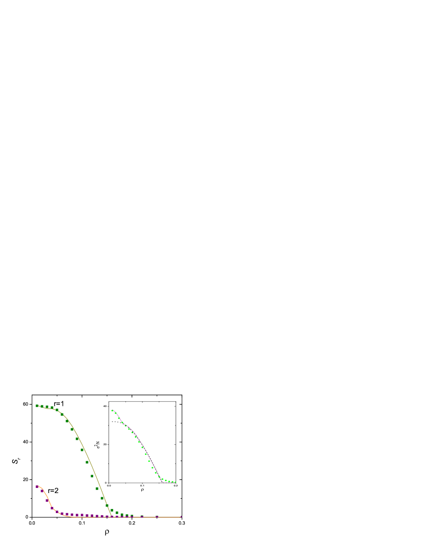
Figure 4: $S_{r}$ versus $\rho$; Inset: $\sigma^{2}/N$ versus $\rho$. Symbols: simulation; dotted line: theory with one bifurcation; solid lines: theory with two bifurcations. $N=1001$, $m=1$, $s=2$, 1000 samples.

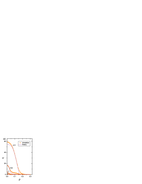
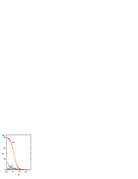
Figure 5: $S_{r}$ versus $\rho$ for (a) $m=2$, (b) $m=3$. In both cases, $N=1001$, $s=2$, 1000 samples.

As shown in Figs. 4-5, the step sizes for each of the $D$ signals do not bifurcate simultaneously at $\rho=\rho_{c}$, Rather, only their first maximum bifurcates from zero when $\rho$ falls below $\rho_{c}$, while the step sizes for the remaining $D$-1 signals remain small. When the diversity further decreases to around 0.05, the second maximum becomes unstable as well, and a further bifurcation takes place. For $m\geq 2$, there are further bifurcations of the third or higher order maxima, resulting in a cascade of dynamical transitions when the diversity decreases.

This cascade of transitions is confirmed by analysis. For $m=1$, we can generalize Eq. (3) to convergence times of the order $\sqrt{R}$. Assuming without loss of generality that $\mathrm{A}^{1}$ bifurcates while $\mathrm{A}^{0}$ remains small, the variance of the buyer population, as derived in Ting2004 , is

$$\frac{\sigma^{2}}{N}=\frac{N}{32}(\Delta\mathrm{A}^{1})^{2},\quad\Delta\mathrm{A}^{1}=\mathrm{erf}\left(\frac{\Delta\mathrm{A}^{1}}{\sqrt{8\rho}}\right),$$ (5)

where $\Delta\mathrm{A}^{1}$ is the step size responding to signal 1. As Fig. 4 inset shows, the analytical and simulation results well agree down to $\rho\sim 0.05$. However, when the diversity decreases further, this simple analysis implies that the variance will saturate to a constant $N/32$, whereas simulation results are clearly higher.

This discrepancy is due to a further bifurcation of the minimum step size. This can be analyzed by considering the effect of a perturbation $\delta\mathrm{A}^{0}(t)$ in the direction of $\mathrm{A}^{0}$. After a period of 4 steps, the accumulated perturbation becomes

$$\delta\mathrm{A}^{0}(t+4)=\left[1-\frac{1}{\sqrt{2\pi\rho}}(1+e^{-\frac{(\Delta\mathrm{A}^{1})^{2}}{8\rho}})\right]^{2}\delta\mathrm{A}^{0}(t).$$ (6)

At $\rho=0.0459$, where $\Delta$A${}^{1}=0.9775$, the coefficient on the right hand side of Eq. (6) reaches the value 1, and $\delta\mathrm{A}^{0}(t)$ diverges on further reduction of $\rho$. Numerical iterations of the analytical equations for $\mathrm{A}^{\mu}(t)$, averaged over samples of different initial conditions, yield the theoretical curves in Fig. 4 and inset, agreeing very well with simulation results. Similarly, the agreement between analytical and simulation results are satisfactory for $m=2$.

Since the attractors have asymmetric responses to different signals, we also study their dependence on the initial states. Letting the system start from a certain state (say, state 1 for $m=1$) for a given sample, Fig. 6 shows that the initial state is more likely to have the largest step size in the attractor for $m=1$. Simulations show that higher values of $m$ share the same trend.

Figure 6: The number of samples with step size responding to signal 1 being the maximum, out of 1000 samples for $N=1001$, $m=1$, and $s=2$. The initial signal is 1.

V Conclusion

We have studied the behavior of an adaptive population using a payoff function that increases linearly with the winning margin. We found a continuous dynamical transition when the adaptation rate of the population is tuned by varying their diversity of preferences. This is in contrast with the case of payoff functions independent of the winning margin, in which no phase transitions are found. Furthermore, we found a cascade of dynamical transitions in the responses to different signals. This shows that an adaptive population has the ability to self-organize to globally efficient states and display a rich behavior, although the individual agents make selfish decisions. Hence, despite the simplicity of the population models, they are able to capture the essential features of economic markets and distributed control.

References

- (1) P. W. Anderson, K. J. Arrow and D. Pines, The Economy as an Evolving Complex System (Addison Wesley, Redwood City, CA, 1988).
- (2) D. Challet, M. Marsili and Y. C. Zhang, Minority Games Physica A, 246, 407 (1997).
- (3) G. Wei and S. Sen, Adaption and learning in multi-agent systems, Lecture Notes in Computer Science 246 (Springer, Berlin, 1995).
- (4) F. Schweitzer (ed.), Modeling Complexity in Economic and Social Systems (World Scientific, Singapore, 2002).
- (5) R. Savit, R. Manuca, and R. Riolo, Phys. Rev. Lett. 82, 2203 (1999).
- (6) R. Manuca, Y. Li, R. Riolo, and R. Savit, Physica A 282, 559 (2000).
- (7) D. Challet, M. Marsili, and R. Zecchina, Phys. Rev. Lett. 84, 1824 (2000).
- (8) M. Marsili, D. Challet, and R. Zecchina, Physica A 280, 522 (2000).
- (9) J. A. F. Heimel, and A. C. C. Coolen, Phys. Rev. E 63, 056121 (2001).
- (10) A. C. C. Coolen, The Mathematical Theory of Minority Games (Oxford University Press, Oxford, UK, 2005).
- (11) Y. Li, A. vandeemen, and R. Savit, Physica A 284, 461 (2000).
- (12) K. Lee, P. M. Hui, and N. F. Johnson, Physica A 321, 309 (2003).
- (13) A. de Martino, I. Giardina, M. Marsili, and A. Tedeschi, Phys. Rev. E 70, 025104(R) (2004).
- (14) K. Y. M. Wong, S. W. Lim, and Z. Gao, Phys. Rev. E 70, 025103(R) (2004).
- (15) K. Y. M. Wong, S. W. Lim, and Z. Gao, Phys. Rev. E 71, 066103 (2005).
- (16) Y. S. Ting, MPhil Thesis, HKUST (2004).