Level-crossing spectroscopy of the 7, 9, and 10D_5/2 states of ¹³³Cs and validation of relativistic many-body calculations of the polarizabilities and hyperfine constants

Abstract

We present an experimental and theoretical investigation of the polarizabilities and hyperfine constants of D_J states in ¹³³Cs for $J=3/2$ and $J=5/2$. New experimental values for the hyperfine constant $A$ are obtained from level-crossing signals of the (7,9,10)D_5/2 states of ¹³³Cs and precise calculations of the tensor polarizabilities $\alpha_{2}$. The results of relativistic many-body calculations for scalar and tensor polarizabilities of the (5-10)D_3/2 and (5-10)$D_{5/2}$ states are presented and compared with measured values from the literature. Calculated values of the hyperfine constants $A$ for these states are also presented and checked for consistency with experimental values.

I Introduction

Level-crossing spectroscopy in an electric field has been shown to be a useful technique to determine atomic properties. Already the first experimental studies of resonant signals at pure electric field crossings of magnetic $\pm m_{F}$ components of certain hyperfine (hfs) atomic levels $F$ at nonzero electric field Khadjavi et al. (1966, 1968); Schmieder et al. (1971) and their further development by applying two-step laser excitation Auzinsh et al. (2006) demonstrated how this technique could be used to obtain atomic properties. The method makes use of the fact that the electric field values at which magnetic sublevels $m_{F}$ cross in an electric field depend on the tensor polarizability $\alpha_{2}$ and on the hfs constants. When the electric field is scanned and laser induced fluorescence (LIF) of definite polarization is observed, these crossings are associated with resonance behavior in the LIF signals. When the separation between crossings is large compared to the widths of the resonance signals, as in the $n$D_3/2 states of the ¹³³Cs atom (see Fig. 1a), they lead to rather well-pronounced resonances in the observed fluorescence. Moreover, these resonances correspond exactly to the level-crossing points under appropriate experimental conditions. Such resonances were used to measure the tensor polarizabilities $\alpha_{2}$ in the $7,9$D_3/2 states of ¹³³Cs atoms Auzinsh et al. (2006), in which the magnetic dipole coupling hfs constant $A$ had been previously measured with good precision, and the electric quadrupole hfs constant $B$ was assumed to be negligibly small Arimondo et al. (1977).

Such measurements become more challenging, however, in the case of the $n$D_5/2 states of cesium, since there are many closely spaced crossing points of magnetic $\pm m_{F}$ components (see Fig. 1,b-d). As a result, the level-crossing signals overlap and no longer contain discernable resonances. In this case, reliable values for atomic properties can be extracted only by means of a very detailed and accurate theoretical description of the observed electric field dependence of the signals as a function of atomic properties and experimental conditions. Such theoretical descriptions have been developed and tested in connection with the $n$D_3/2 states Auzinsh et al. (2006). Nevertheless, the level-crossing technique cannot be used at this time to improve the knowledge of the tensor polarizabilities $\alpha_{2}$ of the $n$D_5/2 states because the extant measurements of the hfs constant $A$ contain uncertainties on the order of 30%. The small hyperfine interaction, especially for $n>7$, makes them difficult to measure Hogervorst and Svanberg (1975); Svanberg and Tsekeris (1975).

The first value of the hfs constant $A$ of the $n$D_5/2 states of ¹³³Cs was obtained with measurements of the widths of optical double resonance (ODR) signals in the Paschen-Back region. The results for the 9D_5/2 and 10D_5/2 states were $-0.5(2)$ MHz and $-0.4(2)$ MHz, respectively Svanberg et al. (1973). These values were improved through level-crossing spectroscopy in magnetic fields, yielding $-0.40(15)$ and $-0.30(10)$ MHz Hogervorst and Svanberg (1975). The authors combined these data with previous ODR measurements Svanberg and Tsekeris (1975) and presented the weighted average as $-0.45(10)$ and $-0.35(10)$ MHz. They concluded that the quadrupole interaction can be completely ignored when fitting the experimental data. For the 7D_5/2 state, Bulos et al. estimated the $A$ value to be $-1.7(2)$ MHz from the ODR signal width Bulos et al. (1976). The drawback of the ODR experiments on the 7,9,10D_5/2 signals is that it is necessary to use indirect cascade transitions to observe the $n$D_5/2 signals because of the presence of scattered light at the $n$D${}_{5/2}\longrightarrow$ 6P_3/2 fluorescence transition Svanberg and Tsekeris (1975); Bulos et al. (1976)

The tensor polarizabilities $\alpha_{2}$ for the $n$D_5/2 states in cesium under discussion are known with far greater precision. For the 10D_5/2 state, $\alpha_{2}$ has been measured by Xia and coworkers to a very high precision of about 0.3% at $6815(20)\times 10^{3}$ a.u. Xia et al. (1997). For the 9D_5/2 state the $\alpha_{2}$ value is measured with ca. 5% accuracy at $2650(140)\times 10^{3}$ a.u. by means of level crossing spectroscopy in combined electric and magnetic fields Hogervorst and Svanberg (1975); Fredriksson and Svanberg (1977). For the 7D_5/2 state, there exists a measured value of $129(4)\times 10^{3}$ a.u. presented in Ref. Wessel and Cooper (1987), which, however, should be verified, because it differs significantly from the theoretical value of $140\times 10^{3}$ a.u. Wijngaarden and Li (1994). Furthermore, a more recent measurement of $\alpha_{2}$ for the 7D_3/2 state Auzinsh et al. (2006) was closer to the theoretical estimate of Wijngaarden and Li (1994) than the measurement of Wessel and Cooper (1987).

The situation with the electronic structure calculations is similar to the experimental situation. Rather good accuracy has been achieved for theoretical estimates of the tensor polarizability $\alpha_{2}$, as can be seen from the fact that the calculations of Wijngaarden and Li (1994) for ¹³³Cs agree with very accurate experimental data for the (10-13)D_3/2,5/2 states Xia et al. (1997). Despite this precision for the polarizability, the estimates of the hfs constants are poor and can hardly be evaluated reliably, for reasons that will be discussed below. Therefore, there is a need for more accurate values for the hfs constants of the $n$D_5/2 states.

In order to determine the hfs constants $A$ from our measurements of $m_{F}$ sublevel crossing signals in the 7,9,10D_5/2 states of cesium, we used the following approach. We fit the measured signals with calculated curves derived from simulations, which had been developed and tested in Auzinsh et al. (2006). With the tensor polarizability $\alpha_{2}$ fixed, these fits yielded the hfs constant $A$. To choose the proper value for $\alpha_{2}$, we performed an all-order relativistic many-body calculation.

Section II contains a description of the experiment, followed by a discussion of the simulations used to describe the measured signals. The all-order relativistic many-body calculations that provided the values for the tensor polarizabilities $\alpha_{2}$ are described in section III, and the values for $\alpha_{2}$ obtained from these calculations are compared with earlier experimentally measured values. In section IV we discuss the application of these calculations to estimating the hfs constants and compare them to the results of previous experiments. In section V we show how to use our experimental results from section II and the calculated tensor polarizabilities from section III to estimate new values for the hfs constant $A$.

II Experiment and Description of Signals

II.1 Method

The premise of level crossing spectroscopy is that the spatial intensity distribution and polarization of the laser induced fluorescence produced when an atom is excited depends on the coherences between different magnetic sublevels $m_{F}$ of hyperfine levels $F$. Such coherences are destroyed when the degeneracy between different sublevels is broken in an electric field. However, in the case of linear polarization, they can be restored when sublevels with $\Delta m_{F}=\pm 2$ cross at certain electric field values. Figure 1 shows the hyperfine level-splitting diagram in an external electric field for the 7D_3/2 and 7D_5/2 states of cesium. This diagram is calculated by diagonalizing the Hamiltonian, which includes the hyperfine and Stark interactions, in an uncoupled basis Aleksandrov et al. (1993).

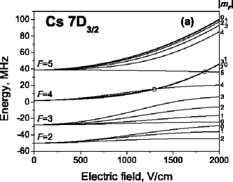
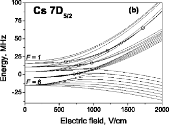
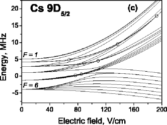
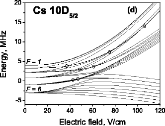
Figure 1: Hyperfine level-splitting diagram in an external electric field for the (a) 7D_3/2, (b) 7D_5/2, (c) 9D_5/2, and (d) 10D_5/2 states of Cs. Circled points indicate level crossings with $\Delta m_{F}=\pm 2$.

When applying the method of level crossing spectroscopy to the study of the $n$D_5/2 states of cesium, one encounters two difficulties not present in the case of the $n$D_3/2 states. The first difficulty is that the $n$D_5/2 hyperfine manifold contains seven level crossings with $\Delta m_{F}=\pm 2$, whereas the $n$D_3/2 manifold contains only two (see Fig. 1). The large number of level crossings in the $n$D_5/2 state wash out the sharp resonances that could be observed in the $n$D_3/2 state.

The second difficulty is that in the case of the $n$D_5/2 states, after the two-step excitation 6S${}_{1/2}\longrightarrow 6$P_3/2 $\longrightarrow n$D_5/2 (see Fig. 2), it is necessary to observe the fluorescence from the $n$D${}_{5/2}\longrightarrow 6$P_3/2 transition. Thus, scattered light from the exciting laser constitutes a high background that must be suppressed. Figure 2 shows the level excitation scheme.

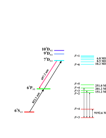
Figure 2: Level excitation scheme.

II.2 Experimental details

We studied cesium vapor at room temperature in a glass cell. The experimental setup is essentially the same as in Ref. Auzinsh et al. (2006). We could apply an electric field between two transparent electrodes inside the cell, which were separated by a 2.5 mm gap. Figure 3 shows a schematic diagram of the experimental setup and geometry. The most crucial detail of the experiment is the relative orientation of the electric field and the polarization vectors of the linearly polarized laser radiation. The first laser, which excited the $6$S${}_{1/2}\longrightarrow 6$P_3/2 transition, was polarized with its polarization vector E₁ parallel to the dc electric field $\mathcal{E}$, which was along the $z$-axis. The second laser, which excited the 6P${}_{3/2}\longrightarrow$ 7,9,10D_5/2 transition, was sent in a counter propagating direction and was polarized perpendicular to the first, with polarization vector E₂ parallel to the $y$-axis. We observed the laser induced fluorescence (LIF) at the $n$D${}_{5/2}\longrightarrow$ 6P_3/2 transition along the $z$-axis through the transparent electrodes. A linear polarizer selected the intensities of the LIF polarization components along the $x$ or $y$-axes $I_{x}$ or $I_{y}$. Since the LIF was observed at the same frequency at which the second laser was operating, it was necessary to suppress carefully the scattered light by means of diaphragms. The scattered light accounted for between 30% and 50% of the measured signal. We checked that this background remained stable during the measurements and subtracted it from the signals. The LIF passed through an MDR-3 monochromator with 2.6 nm/mm inverse dispersion and was recorded with a PMT in photon counting mode during one second time intervals.

The first laser was always a diode laser (based on an LD-0850-100sm laser diode) and was tuned to excite the 6²P_3/2 state from the $F=3$ hfs component of the ground state. We chose to excite from the $F=3$ level, because in this way we could avoid the $F=6$ level of the $n$D_5/2 final state. The $F=6$ level contained no level crossings and thus would contribute only background. We took advantage of a sideband of the radiation of the first laser in order to achieve broadband excitation.

For the second excitation step, we used a diode laser (based on a Hitachi HL6738MG laser diode) in the case of the 7D_5/2 state and a CR699-21 ring dye laser with Rhodamine 6G dye in the case of the 9D_5/2 and 10D_5/2 states. The second laser was operated in single mode regime. We recorded data at different values of the detuning of the second laser in order to compare the results obtained at different detunings with simulations. A HighFinesse WS/6 wavemeter allowed us to measure changes in the lasers’ detuning with a resolution of 30 MHz. However, in general we operated at the detuning that maximized the fluorescence signal. When the second laser was the diode laser, we jittered its output frequency over a range of approximately 1.2 GHz by applying a sawtooth wave with a frequency of tens of Hertz to a piezoelectric crystal mounted to its feedback grating. The laser power was of the order of a few mW, and the laser beam diameters were approximately 1 mm.

The electric field produced in the cell was calibrated with measurements of level-crossing signals for the 10D_3/2 state of cesium as in Auzinsh et al. (2006). The level-crossing resonance positions obtained with our cell were compared with the crossing points calculated from the tensor polarizability of Xia et al. (1997) and the hfs constant $A$ of Arimondo et al. (1977). The overall uncertainty on the electric field magnitude was estimated to be about 1%.

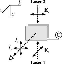
Figure 3: Experimental geometry.

II.3 Experimental results

We plot with markers the measured LIF intensity as a function of the electric field for the $n$D_5/2 states of cesium in Figures 4–6. Signals for different experimental geometries are plotted. We label the experimental geometry as $zyy$ or $zyx$, where the first and the second letters, $z$ and $y$, denote the orientation of the polarization of the first and second lasers, $\mathbf{E_{1}}||z$ and $\mathbf{E_{2}}||y$, and the third letter, $x$ or $y$, denotes the polarization direction of the observed LIF. The solid line in the figure indicates the results of the simulations that are described below. As inputs to the theoretical model, we used the tensor polarizabilities calculated with the relativistic many-body approach described in section III below.

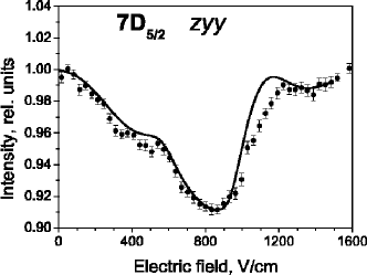
Figure 4: Experimental results for 7D_5/2.

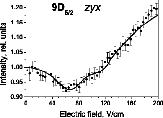
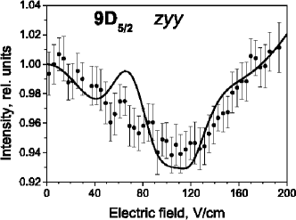
Figure 5: Experimental results for 9D_5/2.

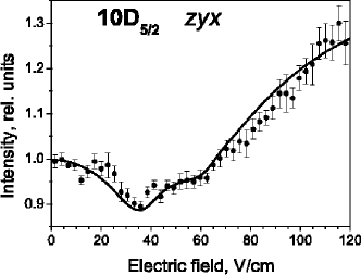
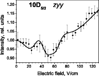
Figure 6: Experimental results for 10D_5/2.

As can be seen from Figures 4, 5, and 6 there are no well-defined level crossing resonances. Nevertheless, a curve with multiple features is obtained, and these features can be fitted with the results of a simulation based on a theoretical model. This simulation is described in the following subsection. The fit involves adjusting the hyperfine constant $A$ and those experimental parameters that we could not measure absolutely, such as the laser detuning. We fix the tensor polarizability $\alpha_{2}$ at the values that are obtained from the calculations described in section III.

II.4 Signal description

Since well-defined resonances are no longer present in the signals of the D_5/2 states, the data can be interpreted only by means of simulations based on a detailed model. Such a model was elaborated in detail and verified in a previous publication Auzinsh et al. (2006), so we will only outline the approach in what follows.

The model describes atoms that interact simultaneously with radiation produced by two lasers with relatively broad spectral profiles, which were necessary to excite coherently magnetic sublevels that are split by an external electric field $\mathcal{E}$ (see Fig. 1). The model assumes that the atoms move classically and are excited at the internal transitions. Thus, the internal atomic dynamics can be described by a semiclassical atomic density matrix $\rho$, which also depends on the classical coordinates of the atomic center of mass.

The ground state of the Cs atom consists of two hyperfine levels with total angular momentum $F_{g}=3$ and $F_{g}=4$, each containing $2F_{g}+1$ magnetic sublevels. The first laser excites the atoms from the ground state to the 6P_3/2 state, which contains hyperfine levels $F_{e}=2,3,4,$ and $5$. The second laser excites the atom from the 6P_3/2 state to the $n$D_5/2 state, which contained hyperfine levels $F_{f}=1,2,3,4,5,$ and $6$.

The external electric field $\mathcal{E}$ partially decouples the electronic angular momentum from the nuclear spin, which implies that the magnetic sublevel energies no longer depend quadratically on the electric field (see Fig. 1). In order to obtain the real dependence on the electric field, it is necessary to diagonalize the full Hamilton matrix. It is also necessary to take into consideration that the decoupling of angular momentum from nuclear spin alters the dipole transition probabilities between magnetic sublevels.

The entire model is based on the Optical Bloch Equations (OBEs) for the density matrix $\rho$ (see, for example, Stenholm (2005))

$$i\hbar\dfrac{\partial\rho}{\partial t}=\left[\widehat{H},\rho\right]+i\hbar\widehat{R}\rho.$$ (1)

The relaxation operator $\widehat{R}$ includes spontaneous emission and transit relaxation. We assume that the density of atoms is sufficiently low that different velocity groups of thermally moving atoms do not interact. The elements of the relaxation matrix are given in Auzinsh et al. (2006). The Hamiltonian $\widehat{H}=\widehat{H}_{hfs}+\widehat{V}$ includes the hyperfine Hamiltonian and the dipole interaction operator $\widehat{V}=-\widehat{\mathbf{d}}\cdot\mathbf{E}\left(t\right)$, where $\widehat{\mathbf{d}}$ is the electric dipole operator and $\mathbf{E}(t)$ is the electric field of the exciting radiation.

The equations can be simplified by assuming that each laser excites only the transition to which it is tuned. We also apply the rotating wave approximation for multilevel systems Arimondo (1996) to the OBEs. The resulting stochastic differential equations can be further simplified by using the decorrelation approach van Kampen (1976). The stochasticity derives from the random fluctuations of the laser radiation with finite spectral width. This approach assumes that both lasers are uncorrelated and that the integration time for each measurement is large compared to the characteristic phase-fluctuation time of the exciting light source. The decorrelation approximation amounts to solving the equations of the density matrix elements that correspond to optical coherences and taking a formal statistical average over the fluctuating phases Blush and Auzinsh (2004). This procedure results in a system of equations that, when solved, yields the observed signals.

From the density matrix of the final state, one can obtain the fluorescence intensities of a given polarization along the unit vector $\mathbf{e}$ from Auzinsh and Ferber (2005); Barrat and Cohen-Tannoudji (1961); Dyakonov (1965):

$$I\left(\mathbf{e}\right)=\widetilde{I}_{0}\underset{g_{i},f_{i},f_{j}}{\sum}d_{g_{i}f_{j}}^{(ob)\ast}d_{e_{i}g_{i}}^{(ob)}\rho_{f_{i}f_{j}},$$ (2)

where $\widetilde{I}_{0}$ is a constant and $d_{g_{i}f_{j}}^{(ob)}=$ $\left\langle g_{i}\left|\mathbf{d}\cdot\mathbf{e}\right|f_{j}\right\rangle$ is the matrix element between the ground and final states of the dipole operator along a specific polarization direction $\mathbf{e}$, i.e., the $x-$ or $y-$ direction.

III Calculation of scalar and tensor polarizabilities

III.1 Motivation

The description of the signals obtained from the experiment described above depends on two atomic properties simultaneously: the hyperfine constant $A$ and the tensor polarizability $\alpha_{2}$. If one of these constants can be known by independent means, the experiment provides a way to determine the other. In this section, we describe an all-order relativistic many-body calculation of the tensor polarizability $\alpha_{2}$. A reliable theoretical estimate of this constant, together with the experimental results of the previous section, can be used to estimate the hyperfine constant $A$, which is difficult to calculate theoretically and has not been measured to high precision for the 7,9, and 10D_5/2 states of cesium.

III.2 Method

The scalar $\alpha_{0}$ and tensor $\alpha_{2}$ polarizabilities of an atomic state $v$ are calculated using formulas

$$\alpha_{0}=\frac{2}{3(2j_{v}+1)}\sum_{n}\frac{\langle n\|D\|v\rangle^{2}}{E_{n}-E_{v}}$$ (3)

$$\alpha_{2} =-4\left(\frac{5j_{v}(2j_{v}-1)}{6(j_{v}+1)(2j_{v}+1)(2j_{v}+3)}\right)^{1/2}$$ (6)

$$\sum_{n}(-1)^{j_{v}+j_{n}+1}\left\{\begin{array}[]{ccc}j_{v}&1&j_{n}\\ 1&j_{v}&2\end{array}\right\}\frac{\langle n\|D\|v\rangle^{2}}{E_{n}-E_{v}},$$

where $D$ is the dipole operator and the formula for $\alpha_{0}$ includes only the valence part of the polarizability. The contribution to $\alpha_{0}$ from the ionic core is negligible for the present calculation (16 $a^{3}_{0}$). The sum over $n$ includes the $nP_{1/2}$, $nP_{3/2}$, and $nF_{5/2}$ states for the calculation of the $D_{3/2}$ polarizabilities in cesium and the $nP_{3/2}$, $nF_{5/2}$, and $nF_{7/2}$ states for the calculation of the $D_{5/2}$ polarizabilities. The sum over the intermediate states $n$ converges rather quickly and only the first few terms need to be calculated accurately. Therefore, we separate the calculation of the polarizabilities into the calculation of the main term $\alpha^{\textrm{main}}$ and the evaluation of the remainder $\alpha^{\textrm{tail}}$. We include the contributions from the following states into the main term: $6P$, $7P$, $8P$, $9P$, $10P$, $11P$, $12P$, $4F$, $5F$, $6F$, $7F$, and $8F$ to calculate the polarizabilities of all $D$ states considered in this paper. We also include the contributions from the $9F$ states into the calculation of the $\alpha^{\textrm{main}}(10D)$. All electric-dipole reduced matrix elements in Eqs. (3, 6) that are needed for the calculation of the main term are calculated using the relativistic all-order method, which is briefly described below. We use experimental energies from Moore (1971) in the main term calculations. We note that the polarizabilities of the $9D$ and $10D$ states are very sensitive to the values of the $9D-10P$ and $10D-11P$ energy differences, respectively, since they are small ($50-100$ cm^-1). We assume that the energies in Ref. Moore (1971) are accurate to all quoted digits. The remainders $\alpha^{\textrm{tail}}$ are small for all sums and are calculated in the Dirac-Hartree-Fock (DHF) approximation.

Table 1: The contributions to scalar and tensor polarizabilities for the $7D_{3/2}$ state in cesium. The corresponding energy differences and the absolute values of the lowest-order (DHF) and final all-order electric-dipole reduced matrix elements are also listed. The energy differences are given in cm^-1. The electric-dipole matrix elements are given in atomic units ($ea_{0}$), and the polarizabilities are given in 10³ $a_{0}^{3}$, where $a_{0}$ is Bohr radius.

Contribution	$nlj$	$Z^{DHF}_{nlj,7D_{3/2}}$	$Z^{\textrm{SD}}_{nlj,7D_{3/2}}$	$E_{nlj}-E_{7D_{3/2}}$	$\alpha_{0}(7D_{3/2})$	$\alpha_{2}(7D_{3/2})$
$\alpha^{\text{main}}(nP_{1/2})$	$6P_{1/2}$	1.628	2.067	-14869.6	-0.011	0.011
	$7P_{1/2}$	4.030	6.580	-4282.2	-0.370	0.370
	$8P_{1/2}$	33.633	31.970	-338.7	-110.4(1.2)	110.4(1.2)
	$9P_{1/2}$	13.535	8.734	1589.4	1.756	-1.756
	$10P_{1/2}$	3.843	2.819	2679.2	0.109	-0.109
	$11P_{1/2}$	2.026	1.537	3355.8	0.026	-0.026
	$12P_{1/2}$	1.324	1.020	3805.0	0.010	-0.010
$\alpha^{\text{tail}}(nP_{1/2})$					0.041	-0.041
$\alpha^{\text{main}}(nP_{3/2})$	$6P_{3/2}$	0.794	0.983	-14315.5	-0.002	-0.002
	$7P_{3/2}$	2.111	3.336	-4101.2	-0.099	-0.079
	$8P_{3/2}$	15.190	14.351	-256.1	-29.4(3)	-23.5(3)
	$9P_{3/2}$	5.590	3.430	1634.1	0.263	0.211
	$10P_{3/2}$	1.642	1.142	2706.1	0.018	0.014
	$11P_{3/2}$	0.872	0.627	3373.2	0.004	0.003
	$12P_{3/2}$	0.572	0.417	3816.9	0.002	0.001
$\alpha^{\text{tail}}(nP_{3/2})$					0.008	0.006
$\alpha^{\text{main}}(nF_{5/2})$	$4F_{5/2}$	9.165	13.027	-1575.4	-3.9(1)	0.79(3)
	$5F_{5/2}$	46.603	43.406	923.7	74.6(1.1)	-14.9(2)
	$6F_{5/2}$	9.074	1.289	2281.9	0.027	-0.005
	$7F_{5/2}$	5.484	1.999	3100.4	0.047	-0.009
	$8F_{5/2}$	3.767	1.695	3631.1	0.029	-0.006
$\alpha^{\text{tail}}(nF_{5/2})$					0.434	-0.087
Total					-66.8(1.6)	71.2(1.2)

The all-order method used here sums infinite sets of many-body perturbation theory terms. We refer the reader to Refs. Blundell et al. (1989, 1991); Safronova et al. (1999) for a detailed description of the approach. Briefly, the wave function of the valence electron $v$ is represented as an expansion

$$|\Psi_{v}\rangle = \left[1+\sum_{ma}\,\rho_{ma}a^{\dagger}_{m}a_{a}+\frac{1}{2}\sum_{mnab}\rho_{mnab}a^{\dagger}_{m}a^{\dagger}_{n}a_{b}a_{a}+\right.$$ (7)

$$+ \left.\sum_{m\neq v}\rho_{mv}a^{\dagger}_{m}a_{v}+\sum_{mna}\rho_{mnva}a^{\dagger}_{m}a^{\dagger}_{n}a_{a}a_{v}\right]|\Phi_{v}\rangle,$$

where $\Phi_{v}$ is the lowest-order atomic state function, which is taken to be the frozen-core Dirac-Hartree-Fock wave function of a state $v$. This lowest-order atomic state function can be written as $|\Phi_{v}\rangle=a_{v}^{\dagger}|0_{C}\rangle,$ where $|0_{C}\rangle$ represent DHF wave function of a closed core. The indices $m$ and $n$ designate excited states and indices $a$ and $b$ designate core states. The equations for the excitation coefficients are solved iteratively until the correlation energy converges to an acceptable accuracy. The excitation coefficients $\rho_{ma}$, $\rho_{mv}$, $\rho_{mnab}$, and $\rho_{mnva}$ are used to calculate the matrix elements, which can be expressed in the framework of the all-order method as linear or quadratic functions of the excitation coefficients. The electric-dipole matrix elements as well as the hyperfine constants are calculated using the same approach. The expansion given by Eq. (7) is restricted to single and double (SD) excitations leading to the omission of certain fourth- and higher-order terms.

Table 2: The contributions to the scalar and tensor polarizabilities for the $7D_{5/2}$ state in cesium. The corresponding energy differences and the absolute values of the lowest-order (DHF) and the final all-order electric-dipole reduced matrix elements are also listed. The energy differences are given in cm^-1. The electric-dipole matrix elements are given in atomic units ($ea_{0}$), and the polarizabilities are given in 10³ $a_{0}^{3}$.

Contribution	$nlj$	$Z^{\textrm{DHF}}_{nlj,7D_{5/2}}$	$Z^{\textrm{SD}}_{nlj,7D_{5/2}}$	$E_{nlj}-E_{7D_{5/2}}$	$\alpha_{0}(7D_{5/2})$	$\alpha_{2}(7D_{5/2})$
$\alpha^{\text{main}}(nP_{3/2})$	$6P_{1/2}$	2.375	2.909	-14336.5	-0.014	0.014
	$7P_{1/2}$	6.303	9.679	-4122.2	-0.554	0.554
	$8P_{1/2}$	45.594	43.210	-277.1	-164.3(1.7)	164.3(1.7)
	$9P_{1/2}$	16.835	10.774	1613.1	1.755	-1.755
	$10P_{1/2}$	4.939	3.555	2685.1	0.115	-0.115
	$11P_{1/2}$	2.623	1.947	3352.3	0.028	-0.028
	$12P_{1/2}$	1.720	1.294	3795.9	0.011	-0.011
$\alpha^{\text{tail}}(nP_{3/2})$					0.047	-0.047
$\alpha^{\text{main}}(nF_{5/2})$	$4F_{5/2}$	2.444	3.471	-1596.4	-0.184	-0.210
	$5F_{5/2}$	12.464	11.660	902.7	3.67(5)	4.20(5)
	$6F_{5/2}$	2.441	0.457	2260.9	0.002	0.003
	$7F_{5/2}$	1.472	0.590	3079.4	0.003	0.003
	$8F_{5/2}$	1.011	0.488	3610.1	0.002	0.002
$\alpha^{\text{tail}}(nF_{5/2})$					0.021	0.024
$\alpha^{\text{main}}(nF_{7/2})$	$4F_{7/2}$	10.925	15.292	-1596.5	-3.6(1)	1.28(4)
	$5F_{7/2}$	55.737	52.145	902.6	73.5(9)	-26.2(3)
	$6F_{7/2}$	10.926	2.049	2260.8	0.045	-0.016
	$7F_{7/2}$	6.588	2.643	3079.3	0.055	-0.020
	$8F_{7/2}$	4.522	2.186	3610.1	0.032	-0.012
$\alpha^{\text{tail}}(nF_{7/2})$					0.416	-0.148
Total					-89.0(1.9)	141.8(1.7)

Table 3: The contributions to scalar and tensor polarizabilities for the $9D_{3/2}$ and $9D_{5/2}$ states in cesium in 10³ $a_{0}^{3}$.

Contribution	$\alpha_{0}(9D_{3/2})$	$\alpha_{2}(9D_{3/2})$
$10P_{1/2}$	-1760(9)	1760(9)
$10P_{3/2}$	-483(2)	-386(2)
$6F_{5/2}$	-129(2)	25.8(4)
$7F_{5/2}$	938(8)	-188(2)
Other	31	-22
Total	-1403(12)	1190(10)
Contribution	$\alpha_{0}(9D_{5/2})$	$\alpha_{2}(9D_{5/2})$
$10P_{3/2}$	-2653(12)	2653(12)
$7F_{5/2}$	46.3(3)	53.0(4)
$6F_{7/2}$	-117(2)	41.9(6)
$7F_{7/2}$	927(6)	-331(2)
Other	20	-30
Total	-1777(14)	2386(13)

We use B-splines Johnson et al. (1998) to generate a complete set of DHF basis orbitals for the all-order calculation. Here, we use $N=70$ splines for each angular momentum. The basis orbitals are constrained to a cavity of radius $R=220$ a.u. The size of the cavity is taken to be large enough to fit all of the states needed for the calculation of the main terms for all of the polarizabilities calculated in this work. The calculation of the polarizabilities of the $9D$ and $10D$ states requires such a large cavity since we need to be able to properly describe states up to $12P$ and $9F$. This work required extensive study of the numerical accuracy and stability of the calculations. We verified that our basis set gives correct lowest-order (DHF) values for the energies of all relevant states and transition matrix elements between these states. We have also verified that our basis set correctly reproduces DHF values of the hyperfine constants for all the $nD_{J}$ states considered here. We find that it is necessary to use 70 splines to produce an accurate basis set. We also conducted an all-order calculation with a smaller cavity ($R=90$ a.u.) that is appropriate for the calculation of the properties of the low-lying states and found that the properties of the low-lying states are accurately described by our large $R=220$ a.u., $N=70$ basis set. Therefore, we conclude that numerically accurate results can be obtained even for such highly-excited states as $12P$ with the use of large basis sets.

III.3 Results

The contributions to the scalar and tensor polarizabilities for the $7D_{3/2}$ state in cesium are listed in Table 1. We note that the calculation of the scalar and tensor polarizability differs only in the angular factor, and all matrix elements and energies are the same. The corresponding energy differences and the absolute values of the lowest-order and final all-order electric-dipole reduced matrix elements are also listed. The energy differences are given in cm^-1. Electric-dipole matrix elements are given in atomic units ($ea_{0}$), and polarizabilities are given in 10³ $a_{0}^{3}$, where $a_{0}$ is the Bohr radius. The difference between the lowest-order values and the all-order values allows to evaluate the size of the correlation correction. The accuracy of our calculation is generally higher when the relative size of the correlation correction is smaller.

The contributions from all terms in $\alpha^{\textrm{main}}$ are listed separately to identify the most important terms. The remainder $\alpha^{\textrm{tail}}$ is separated to $\alpha^{\textrm{tail}}(nP_{1/2})$, $\alpha^{\textrm{tail}}(nP_{3/2})$, and $\alpha^{\textrm{tail}}(nF_{5/2})$ for the study of the convergence of these three sums.

We find that three contributions, from the $8P_{1/2}$, $8P_{3/2}$, and $5F_{5/2}$ states, are dominant. Another term ($4F_{5/2}$) gives a small but significant contribution to the tensor polarizability. Therefore, we conduct a more accurate calculation of the relevant matrix elements and evaluate their uncertainties. The study of the breakdown of the correlation correction demonstrates that the main contributions to these transitions come from the terms containing only single valence excitation coefficients $\rho_{mv}$ (see Eq. (7)). In such cases, it is possible to use a semi-empirical scaling procedure such as is described, for example, in Ref. Blundell et al. (1991) to estimate dominant classes of the omitted higher-order corrections. The single excitation coefficients $\rho_{mv}$ are multiplied by the ratio of the experimental and theoretical correlation energy, and the calculation of the matrix elements is repeated using the modified excitation coefficients. The difference between the ab initio and scaled SD all-order values for the particular matrix element is taken to be its uncertainty. The relative uncertainty of the corresponding contribution to polarizability is twice the relative uncertainty of the matrix element. As we noted above, we assume that the experimental energies are accurate to all digits quoted in Ref. Moore (1971). The uncertainties of the total polarizability values are obtained by adding the uncertainties of the individual terms in quadrature. The uncertainty in all remaining contributions is estimated to be insignificant in comparison with the uncertainty of the dominant terms.

Table 4: Contributions to the scalar and tensor polarizabilities for the $10D_{3/2}$ and $10D_{5/2}$ states in cesium in 10³ $a_{0}^{3}$.

Contribution	$\alpha_{0}(10D_{3/2})$	$\alpha_{2}(10D_{3/2})$
$11P_{1/2}$	-4995(24)	4995(24)
$11P_{3/2}$	-1379(6)	-1103(5)
$7F_{5/2}$	-425(2)	85.1(4)
$8F_{5/2}$	2478(16)	-496(3)
Other	84	-65
Total	-4236(29)	3416(24)
Contribution	$\alpha_{0}(10D_{5/2})$	$\alpha_{2}(10D_{5/2})$
$11P_{3/2}$	-7553(31)	7553(31)
$8F_{5/2}$	122(1)	140(1)
$7F_{7/2}$	-386(3)	138(1)
$8F_{7/2}$	2450(17)	-875(6)
Other	51	-89
Total	-5316(36)	6867(32)

We observe significant cancellations between the dominant terms for both scalar and tensor polarizabilities of the $7D_{3/2}$ state. However, the cancellation is more severe for the scalar polarizability, where the contributions from $8P_{1/2}$ and $5F_{5/2}$ states are comparable in size but have opposite signs. Therefore, we expect higher accuracy of our tensor polarizability calculation in comparison with the scalar one.

The contributions to scalar and tensor polarizabilities for the $7D_{5/2}$ state in cesium are listed in Table 2. The table is structured in exactly the same way as the one for the $7D_{3/2}$ state. We find that the contribution from the $8P_{3/2}$ state is clearly dominant and the cancellation is much less severe. For the tensor polarizability, the next largest term, $5F_{7/2}$, is six times as small as the dominant term. The accuracy of the matrix elements in the dominant terms is similar for the $7D_{3/2}$ and $7D_{5/2}$ states. Therefore, our calculation of the $7D_{5/2}$ polarizabilities is expected to be more accurate than that of the $7D_{3/2}$ polarizabilities.

Table 5: Comparison of the scalar polarizabilities $\alpha_{0}$ for the $7D$, $9D$, and $10D$ states in cesium with other theory and experiment. The polarizabilities are given in 10³ $a_{0}^{3}$.

State	This work	Expt.	Ref. Wijngaarden and Li (1994)
$7D_{3/2}$	-66.8(1.6)	-60(8)  Wessel and Cooper (1987)	-65.2
$9D_{3/2}$	-1403(12)	-1450(120) Fredriksson and Svanberg (1977)	-1400
$10D_{3/2}$	-4236(29)	-4185(4)  Xia et al. (1997)	-4220
$7D_{5/2}$	-89.0(1.9)	-76(8)  Wessel and Cooper (1987)	-87.1
$9D_{5/2}$	-1777(14)	-2050(100) Fredriksson and Svanberg (1977)	-1770
$10D_{5/2}$	-5316(36)	-5303(8)  Xia et al. (1997)	-5300

Table 6: Comparison of the tensor polarizabilities $\alpha_{2}$ for the $7D$, $9D$, and $10D$ states in cesium with other theory and experiment. The polarizabilities are given in 10³ $a_{0}^{3}$.

State	This work	Expt.	Ref. Wijngaarden and Li (1994)
$7D_{3/2}$	71.2(1.2)	74.5(2.0) Auzinsh et al. (2006)	70.4
		66(3) Wessel and Cooper (1987)
$9D_{3/2}$	1190(10)	1183(35) Auzinsh et al. (2006)	1190
		1258(60)  Fredriksson and Svanberg (1977)
$10D_{3/2}$	3416(24)	3401(4) Xia et al. (1997)	3410
$7D_{5/2}$	141.8(1.7)	129(4) Wessel and Cooper (1987)	140
$9D_{5/2}$	2386(13)	2650(140)  Fredriksson and Svanberg (1977)	2380
$10D_{5/2}$	6867(32)	6815(20)  Xia et al. (1997)	6850

The contributions to scalar and tensor polarizabilities for the $9D_{J}$ and $10D_{J}$ states in cesium are listed in Tables 3 and  4, respectively. The breakdown of the polarizability contributions is similar to that of the $7D$ polarizability calculations. We list only the dominant contributions separately and group all of the other contributions together in the rows labeled “Other”. The uncertainty is evaluated using the method described above. The relative importance of the correlation corrections decreases with the principal quantum number $n$ and the cancellation of different terms becomes less significant resulting in smaller uncertainties of the polarizabilities for the $9D$ and $10D$ states in comparison with the uncertainties for the $7D$ states. Overall, the uncertainties of our polarizability calculation are $0.5\%-2.3\%$.

III.4 Comparison with existing experimental values and other theory

Our results for the scalar polarizabilities of the $7D_{J}$, $9D_{J}$, and $10D_{J}$ states in cesium are compared with the experimental values from Refs. Wessel and Cooper (1987); Fredriksson and Svanberg (1977); Xia et al. (1997) and theoretical values from Ref. Wijngaarden and Li (1994) in Table 5. The polarizabilities are given in 10³ $a_{0}^{3}$. The conversion factor from the MHz/(kV/cm)² units to $10^{3}$ atomic units used in the present work is $10^{-7}h/(4\pi\epsilon_{0}a_{0}^{3})=4.01878$, where $h$ is the Planck constant. The present values agree with the experimental results for $7D_{3/2}$, $9D_{3/2}$, and $10D_{5/2}$ states within the corresponding uncertainties. There is some discrepancy with the accurate experimental value for the $10D_{3/2}$ state, but the discrepancy is only 1.5 of our estimated uncertainty. However, our values for the $7D_{5/2}$ and $9D_{5/2}$ states disagree significantly with the experimental values for these states. The calculations for the 7D_5/2, 9D_5/2, and 10D_5/2 state polarizabilities are very similar. Thus, the experimental values for the scalar polarizabilities are not consistent with each other according to our theoretical model. Our calculations confirm the value for the 10D_5/2 state to high precision, and one would have expected similar agreement in the case of the 7D_5/2 and 9D_5/2 state.

The results for the tensor polarizabilities for the $7D_{J}$, $9D_{J}$, and $10D_{J}$ states in cesium are compared with the experimental values from Refs. Wessel and Cooper (1987); Fredriksson and Svanberg (1977); Xia et al. (1997); Auzinsh et al. (2006) and theoretical values from Ref. Wijngaarden and Li (1994) in Table 6. The polarizabilities are also given in 10³ $a_{0}^{3}$. The present results for the $nD_{3/2}$ states support the measurements of Refs. Xia et al. (1997); Auzinsh et al. (2006) and disagree with the less precise previous measurements Wessel and Cooper (1987); Fredriksson and Svanberg (1977). The comparison of the $nD_{5/2}$ values with experiment mirrors the result of the comparison for the scalar polarizabilities: the $7D_{5/2}$ and $9D_{5/2}$ values differ significantly from the experiment while the $10D_{5/2}$ value agrees with the precise experiment within the corresponding uncertainties. Our values agree with the calculation of Ref. Wijngaarden and Li (1994) for all states for both scalar and tensor polarizabilities.

Table 7: The breakdown of the correlation correction to the hyperfine constants $A$ for the $nD_{3/2}$ and $nD_{5/2}$ states in cesium calculated using the SD all-order method. The expressions for all terms are given in Blundell et al. (1989). The values of the contributions for the dominant terms and total correlation correction are given in $\%$ relative to the lowest-order value for each state. The total contains contributions from all terms ($a-t$). The normalization factor is also listed.

Contribution	$5D_{3/2}$	$6D_{3/2}$	$7D_{3/2}$	$8D_{3/2}$	$9D_{3/2}$	$10D_{3/2}$
Term a	11%	26%	28%	28%	28%	28%
Term c	127%	57%	36%	28%	23%	21%
Term d	41%	9%	4%	2%	2%	1%
Term h	13%	9%	5%	4%	3%	3%
Term p	19%	13%	11%	10%	9%	9%
Total	214%	118%	87%	75%	69%	65%
Norm	1.10	1.14	1.12	1.10	1.10	1.09
Contribution	$5D_{5/2}$	$6D_{5/2}$	$7D_{5/2}$	$8D_{5/2}$	$9D_{5/2}$	$10D_{5/2}$
Term a	-352%	-264%	-228%	-213%	-205%	-200%
Term c	120%	54%	35%	27%	23%	21%
Term d	37%	8%	3%	2%	2%	1%
Term h	-154%	-28%	-5%	3%	6%	8%
Term n	18%	16%	14%	13%	12%	12%
Term p	13%	10%	9%	8%	8%	8%
Term r	-24%	-18%	-15%	-14%	-14%	-13%
Total	-339%	-217%	-184%	-171%	-164%	-160%
Norm	1.09	1.12	1.10	1.09	1.09	1.08

IV Calculation of Hyperfine constants

In this section we evaluate the current knowledge about the hyperfine constants of the D_3/2 and D_5/2 states of cesium. We describe a calculation of the hyperfine constants for the $5D_{3/2}-10D_{3/2}$ and $5D_{5/2}-10D_{5/2}$ states of ¹³³Cs. Then we compare the results of the calculation to previously measured values. The calculation of the hyperfine constants also makes use of the relativistic all-order method and is done in the same way as the calculation of the electric-dipole matrix elements and with the same set of the excitation coefficients $\rho_{ma}$, $\rho_{mv}$, $\rho_{mnab}$, and $\rho_{mnva}$ (see Eq. (7) ). The breakdown of the correlation correction to the hyperfine constants $A$ for $nD_{3/2}$ and $nD_{5/2}$ states in cesium calculated using the SD all-order method is given in Table 7. The expressions for the Terms $a,c,d,h,n,$ and $p$ are given in Blundell et al. (1989). These terms are linear or quadratic functions of the excitation coefficients. The values of the contributions of the dominant terms and total correlation correction are given in $\%$ relative to the lowest-order value for each state. The normalization factor is also listed. We find that the correlation correction is very large, especially for the $D_{5/2}$ states where it is several times as large as the lowest-order value and has an opposite sign. Owing to such an enormous correlation correction, we do not expect our results to be very accurate for the $nD_{5/2}$ states. The scaling procedure described above or partial ab initio inclusion of the triple excitation as described in Ref. Safronova et al. (1999) can only evaluate corrections to terms $c$ and $d$, that are not dominant for any of the states except $5D_{3/2}$. Therefore, we can not make an accurate estimate of the uncertainty of our values that is independent from experimental measurements.

Table 8: The hyperfine constants $A$ (MHz) for the $nD_{3/2}$ and $nD_{5/2}$ states in cesium. The lowest-order, “dressed” third-order values, and all-order values are compared with previous experiments. The experimental data are taken from  Arimondo et al. (1977).

State	DHF	Third order	All order	Expt. Arimondo et al. (1977)
$5D_{3/2}$	18.2	47.0	52.3	48.78(7)
$6D_{3/2}$	9.27	21.5	17.8	16.30(15)
$7D_{3/2}$	4.70	10.1	7.88	7.4(2)
$8D_{3/2}$	2.65	5.46	4.20	3.94(8)
$9D_{3/2}$	1.63	3.28	2.51	2.35(4)
$10D_{3/2}$	1.07	2.12	1.62	1.51(2)
$5D_{5/2}$	7.47	-32.3	-16.4	-21.24(8)
$6D_{5/2}$	3.73	-8.15	-3.89	-3.6(10)
$7D_{5/2}$	1.88	-2.67	-1.42	-1.7(2)
$8D_{5/2}$	1.06	-1.15	-0.684	-0.85(20)
$9D_{5/2}$	0.651	-0.592	-0.384	-0.45(10)
$10D_{5/2}$	0.428	-0.343	-0.238	-0.35(10)

Table 9: The consistency check of the experimental hyperfine constants $A$ (MHz) values for the $nD_{3/2}$ and $nD_{5/2}$ states in cesium. The actual experimental data from Ref. Arimondo et al. (1977) are listed in the second column. The columns labeled “S($nD_{J}$)”, $n=6-10$, give data obtained by taking the experimental value for this particular $nD_{J}$ state and rescaling it for all the other states using the theoretical values for the correlation correction as explained in the text. The uncertainty of the rescaled values comes only from the experimental uncertainty of the initial experimental value $nD_{J}$.

State	Expt. Arimondo et al. (1977)	S($6D_{3/2}$)	S($7D_{3/2}$)	S($8D_{3/2}$)	S($9D_{3/2}$)	S($10D_{3/2}$)
$6D_{3/2}$	16.30(15)		16.5(5)	16.3(4)	16.2(4)	16.1(3)
$7D_{3/2}$	7.4(2)	7.33(6)		7.35(16)	7.3(1)	7.25(12)
$8D_{3/2}$	3.94(8)	3.93(3)	4.0(1)		3.92(7)	3.89(6)
$9D_{3/2}$	2.35(4)	2.36(2)	2.38(6)	2.36(5)		2.33(3)
$10D_{3/2}$	1.51(2)	1.53(1)	1.54(4)	1.53(3)	1.52(3)
State	Expt.	S($6D_{5/2}$)	S($7D_{5/2}$)	S($8D_{5/2}$)	S($9D_{5/2}$)	S($10D_{5/2}$)
$6D_{5/2}$	-3.6(10)		-4.5(5)	-4.6(7)	-4.4(7)	-5.2(1.1)
$7D_{5/2}$	-1.7(2)	-1.3(4)		-1.7(4)	-1.6(3)	-2.0(5)
$8D_{5/2}$	-0.85(20)	-0.6(2)	-0.83(10)		-0.80(17)	-0.97(26)
$9D_{5/2}$	-0.45(10)	-0.34(14)	-0.47(6)	-0.48(11)		-0.56(16)
$10D_{5/2}$	-0.35(10)	-0.21(9)	-0.29(4)	-0.30(8)	-0.28(6)

Our results for the hyperfine constants $A$ (MHz) for the $nD$ state in Cs are compared with previous experiments in Table 8. We list the lowest-order and “dressed” third-order values together with the SD all-order values. The “dressed” third-order calculation has all lowest-order matrix elements replaced by “dressed” matrix elements calculated in the random-phase approximation (RPA) Savukov and Johnson (2000). We find large discrepancies between the third-order and all-order results indicating very large contributions from the fourth- and higher-order terms. Taking into account the very large size of the correlation correction and obviously large contributions from higher orders, we find that the agreement of the all-order calculation with measured values is remarkably good.

We have investigated the issue of the consistency of the experimental hyperfine data using our calculation. Table 7 demonstrates that the breakdown of the correlation for the $6D-10D$ states is rather similar, especially for $nD_{3/2}$ states. We note that $nD_{3/2}$ and $nD_{5/2}$ states have to be considered separately. The distributions of the correlation for both $5D_{3/2}$ and $5D_{5/2}$ states are clearly very different from the ones for the other $nD$ states, and these states are omitted from the consistency check below. For the $nD_{5/2}$ states, the relative contribution of Term $h$ changes sign; however, the contribution from this term is small in comparison with the experimental uncertainty. To cross-check the experimental data, we take the experimental value for one particular $nD_{J}$ state and rescale it for all the other states with the same $J$ using the theoretical values of the correlation corrections. The correlation correction is calculated as the difference between the final (experimental or theoretical) number and the lowest-order DHF value. For example, we take the experimental value $A^{\textrm{Expt}}_{6D_{3/2}}$ and determine how much we need to scale our theoretical correlation correction for the $6D_{3/2}$ state to obtain this value. The scaling factor is defined as

$$S(6D_{3/2})=\frac{A^{\textrm{Expt}}_{6D_{3/2}}-A^{\textrm{DHF}}_{6D_{3/2}}}{A^{\textrm{SD}}_{6D_{3/2}}-A^{\textrm{DHF}}_{6D_{3/2}}},$$

where $A^{\textrm{DHF}}$ and $A^{\textrm{SD}}$ are the lowest-order and all-order values from Table 8 for the $6D_{3/2}$ state. Next, we take our theoretical value for another state, for example, $7D_{3/2}$, and rescale its correlation correction contribution using the scaling factor $S(6D_{3/2})$:

$$A(7D_{3/2})=S(6D_{3/2})\times\left(A^{\textrm{SD}}_{7D_{3/2}}-A^{\textrm{DHF}}_{7D_{3/2}}\right)+A^{\textrm{DHF}}_{7D_{3/2}}.$$ (8)

Then, we calculate $A(8D_{3/2}),A(9D_{3/2})$, and $A(10D_{3/2})$ using Eq. (8). We list these values in the column labeled $S(6D_{3/2})$ of Table 9 which indicates that these values were obtained with the scaling factor $S(6D_{3/2})$. We repeat the procedure using other $nD_{3/2}$ values to define the scaling factor. The uncertainty of the rescaled values comes only from the experimental uncertainty of the initial experimental value $A^{\textrm{Expt}}_{nD_{J}}$. We find that all results in each row are consistent within the uncertainties, leading to the conclusion that the experimental results are internally consistent. We note that such a procedure will not be able to detect a systematic shift of all the experimental results. Since we cannot accurately evaluate the uncertainty of the scaling procedure itself, it is unclear if it can yield data that are more accurate than the corresponding experimental data, even though some of the rescaled data has smaller uncertainties than the actual experimental data. The accuracy of the rescaling is expected to be higher when $\Delta n$ between the original and scaled state is the smallest.

V Analysis of Experimental Data and Estimate of the Hyperfine Constants

The theoretical calculations of the hyperfine constants described in the previous section as well as the experimental measurements of Arimondo et al. (1977) contained large uncertainties. The scaling procedure seems to indicate that the experimental values of the review Arimondo et al. (1977), although taken from different sources, are consistent with each other. Thus, there is an indication that the scaling procedure could yield slightly more accurate predictions of hyperfine constants of states in adjacent levels if the hyperfine constant of one state is known. The experiment described in Section II could provide an independent cross-check of these findings.

With the tensor polarizabilities calculated in section III, the simulations described in section II can be used to estimate the hyperfine constant. First, we calculate a series of simulated curves, varying those experimental parameters that we cannot measure precisely, in particular the detuning of the lasers. When the overall shape of the simulated curve matches the experiment, the positions of the features depend on the values of the tensor polarizability $\alpha_{2}$ and the hyperfine constant $A$.

We assume that the tensor polarizabilities calculated in section III for the 7,9, and 10D_5/2 states of cesium are the most accurate values available because of the excellent agreement between the calculated and previously measured values for the 10D_3/2 state of cesium. By fixing the tensor polarizability at the calculated value in our simulations, we can thus estimate the hyperfine constant A from the level-crossing signals in Figures 4, 5, and 6.

Table 10 summarizes the polarizabilities used in the simulations and the hyperfine values $A$ obtained after a fit to the experimental data.

Table 10: Comparison of the experimentally obtained hyperfine constants with previous experiments and the theory presented in this work

Cesium	Calulated	hyperfine constant
atomic	tensor	(MHz)
state	polarizability	This work	Previous	Theory
	$(10^{3}a_{0}^{3})$		experiment
7D5/2	141.8(1.7)	-1.56(9)	-1.7(2) Arimondo et al. (1977)	-1.42
9D5/2	2386(13)	-0.43(4)	-0.45(10) Arimondo et al. (1977)	-0.384
10D5/2	6867(32)	-0.34(3)	-0.35(10) Arimondo et al. (1977)	-0.238

Considering the difficulty in calculating the hfs constants, the results of the relativistic many-body calculation for the hyperfine constant $A$ agree reasonably well with the experimental measurements for the 7D_5/2 and 9D_5/2 states (within $\sim 1.5\sigma$). The large discrepancy in the case of the 10D_5/2 state seems problematic, since the calculations should be internally consistent, if not completely reliable in absolute terms. This inconsistency could indicate that we slightly underestimated our uncertainties. It is also possible that the self-consistency check is less reliable in the case of the $n$D_5/2 states, because the DHF term and the all order term differ even in their sign.

VI Conclusion

We obtained new values for the hfs constants $A$ of the 7,9, and 10D_5/2 states. Our values agreed with previously measured values, but achieved greater precision. The values were obtained by means of measured level-crossing signals, a detailed theoretical description of these signals, and values for the tensor polarizability calculated with an all-order relativistic many-body method. We demonstrated the all-order relativistic many-body method’s reliability even in highly excited states of ¹³³Cs by comparing scalar and tensor polarizabilities obtained by this method with previously experimentally measured values for the 7,9,10D_3/2 and 7,9,10D_5/2 states of ¹³³Cs.

Our calculated polarizability values were in good agreement with experiment except for the 7 and 9D_5/2 states. However, the experimental values reported for these states are called into question by the fact that values reported in the same works for the 7D_3/2 Wessel and Cooper (1987) and 9D_3/2 Fredriksson and Svanberg (1977) states also disagree with our calculations, whereas more recent measurements of the 7 and 9D_3/2 states Auzinsh et al. (2006) support our calculation, as well as previous calculations Wijngaarden and Li (1994). The method was further applied to calculate values for the hyperfine constants $A$ in the 5-10D_3/2 and 5-10D_5/2 states. Although the calculation cannot be considered reliable in absolute terms, nevertheless they agreed reasonably well in the case of the 7D_5/2 and 9D_5/2 states. For the 10D_5/2 state, the agreement was not as good.