Systematic Characterization of Low Frequency Electric and Magnetic Field Data Applicable to Solar Orbiter

Abstract

We present a systematic and physically motivated characterization of incoherent or coherent electric and magnetic fields, as measured for instance by the low frequency receiver on-board the Solar Orbiter spacecraft. The characterization utilizes the $36$ auto/cross correlations of the $3+3$ complex Cartesian components of the electric and magnetic fields; hence, they are second order in the field strengths and so have physical dimension energy density. Although such $6\times 6$ correlation matrices have been successfully employed on previous space missions, they are not physical quantities; because they are not manifestly space-time tensors. In this paper we propose a systematic representation of the $36$ degrees-of-freedom of partially coherent electromagnetic fields as a set of manifestly covariant space-time tensors, which we call the Canonical Electromagnetic Observables (CEO). As an example, we apply this formalism to analyze real data from a chorus emission in the mid-latitude magnetosphere, as registered by the STAFF-SA instrument on board the Cluster-II spacecraft. We find that the CEO analysis increases the amount of information that can be extracted from the STAFF-SA dataset; for instance, the reactive energy flux density, which is one of the CEO parameters, identifies the source region of electromagnetic emissions more directly than the active energy (Poynting) flux density alone.

1 Background

When analyzing time varying electric and magnetic vector field data from spacecraft, it is common to construct a $6\times 6$ matrix from the complex sixtor $(\mathbf{{E}},\mathbf{{B}})$. In a Cartesian coordinate system, this matrix can be written

$$\left(\begin{array}[]{cccccc}|E_{x}|^{2}&E_{x}E_{y}^{\star}&E_{x}E_{z}^{\star}&E_{x}B_{x}^{\star}&E_{x}B_{y}^{\star}&E_{x}B_{z}^{\star}\\ E_{y}E_{x}^{\star}&|E_{y}|^{2}&E_{y}E_{z}^{\star}&E_{y}B_{x}^{\star}&E_{y}B_{y}^{\star}&E_{y}B_{z}^{\star}\\ E_{z}E_{x}^{\star}&E_{z}E_{y}^{\star}&|E_{z}|^{2}&E_{z}B_{x}^{\star}&E_{z}B_{y}^{\star}&E_{z}B_{z}^{\star}\\ B_{x}E_{x}^{\star}&B_{x}E_{y}^{\star}&B_{x}E_{z}^{\star}&|B_{x}|^{2}&B_{x}B_{y}^{\star}&B_{x}B_{z}^{\star}\\ B_{y}E_{x}^{\star}&B_{y}E_{y}^{\star}&B_{y}E_{z}^{\star}&B_{y}B_{x}^{\star}&|B_{y}|^{2}&B_{y}B_{z}^{\star}\\ B_{z}E_{x}^{\star}&B_{z}E_{y}^{\star}&B_{z}E_{z}^{\star}&B_{z}B_{x}^{\star}&B_{z}B_{y}^{\star}&|B_{z}|^{2}\end{array}\right)$$

This electromagnetic (EM) sixtor matrix has in various guises, such as Wave-distribution functions (WDF) Storey:1974 and so on, been useful in the analysis of EM vector field data from spacecraft, such as on the Cluster and Polar missions. Although this matrix-form description of the second order properties of the EM fields can in some instances be convenient and intuitive, it unfortunately has no real motivation in physics, since physical quantities such as EM fields are ultimately not sixtors.

The EM sixtor matrix lists all possible auto and cross correlations of $\mathbf{{E}}(\mathbf{{x}},t)$ and $\mathbf{{B}}(\mathbf{{x}},t)$ and, hence, contains the complete information of the second order properties of EM waves. It is clear that one obtains the EM energy density $|\mathbf{{E}}|^{2}+|\mathbf{{B}}|^{2}$ by taking the trace of the EM sixtor matrix but it is not clear what other EM quantities can be extracted and how this extraction should be performed in general. Some EM quantities are obvious and can be picked out by hand, such as the Lagrangian density $|\mathbf{{E}}|^{2}-|\mathbf{{B}}|^{2}$, the Poynting flux density $\Re\{\mathbf{{E}}\times\bar{\mathbf{{B}}}\}$, etc; $\bar{\mathbf{{B}}}$ denotes the complex conjugate of $\mathbf{{B}}$, etc. Other EM quantities are not so easily identified. Furthermore, as it stands here, the EM sixtor matrix is a mixture of both scalar and pseudo scalar components. This is due to $\mathbf{{E}}$ being a proper (polar) vector and $\mathbf{{B}}$ being a pseudo (axial) vector. This could be remedied by for instance using the sixtor $(\mathbf{{E}},\pm\mathbf{i}\mathbf{{B}})$ but then again, it is unclear what sign to use for the imaginary unit, $\mathbf{i}$. Regardless of how the sign of $\mathbf{i}$ is chosen one would need to redefine the EM quantities. The trace of the modified proper EM sixtor matrix would in this case correspond to the Lagrangian density rather than the EM energy density, which in turn would have to be redefined. Other EM quantities would also need to be redefined in non-standard ways.

Perhaps even more important for space borne observations: the EM sixtor matrix is not covariant according to the requirements of special relativity. Spacecraft are constantly moving and often spinning observation platforms. EM wave measurements become Doppler shifted and data must often be “despun”. For the $3\times 3$ sub-matrices, $\mathbf{{E}}\otimes\bar{\mathbf{{E}}}$, $\mathbf{{E}}\otimes\bar{\mathbf{{B}}}$, $\mathbf{{B}}\otimes\bar{\mathbf{{E}}}$, and $\mathbf{{B}}\otimes\bar{\mathbf{{B}}}$, where $\otimes$ denote the direct product, despinning is straight forward by applying rotation matrices $\bf{\sf{{R}}}$ from left and $\bf{\sf{{R}}}^{\rm{T}}$ from right, e.q. $\mathbf{{E}}^{\prime}\otimes\bar{\mathbf{{E}}}^{\prime}=\bf{\sf{{R}}}\mathbf{{E}}\otimes\bar{\mathbf{{E}}}\bf{\sf{{R}}}^{\rm{T}}$. To rotate the full EM sixtor matrix, similar operations must be performed four times. This is awkward and the resulting $6\times 6$ matrix is still not covariant. For EM wave measurements in space plasma the last remark can be crucial.

A Lorentz boost is the translation from one Lorentz frame to another one moving at velocity $\mathbf{{v}}$. A Lorentz boost does not necessarily imply relativistic speeds, which is a common misconception; and therefore it do not by itself preclude what is typically associated with relativistic effects. It is simply a quite general recipe to make two different observers agree on a physical observation. The Lorentz boost of the EM field vectors can be written $\mathbf{{E}}^{\prime}=\gamma(\mathbf{{E}}+\mathbf{{v}}\times\mathbf{{B}})$ and $\mathbf{{B}}^{\prime}=\gamma(\mathbf{{B}}-\mathbf{{v}}\times\mathbf{{E}}/c^{2})$, where $c$ is the speed of light and $\gamma=1/\sqrt{1-v^{2}/c^{2}}$. As a matter of fact, the Lorentz boost is the essence of the well-known frozen-in field line theorem from magnetohydrodynamics (MHD); a theory which is commonly used to model the solar wind plasma. In a plasma, relativity comes into play at very a fundamental level since the electromagnetic (Lorentz) force dominates the vast majority of all plasma interactions.

Another example illustrates the problem to separate time (frequency) and space (wave vector) in EM wave observations on board a spacecraft. Assume that we observe a wave mode which is described by an angular frequency $\omega$ and wave vector $\mathbf{{k}}$. We can write this as a 4-vector $(\omega,c\mathbf{{k}})$. Let’s make a Lorentz boost in the $\mathbf{{v}}$ direction:

$$\omega^{\prime} = \gamma(\omega-\mathbf{{k}}\cdot\mathbf{{v}})$$ (6)

$$c\mathbf{{k}}^{\prime} = c\mathbf{{k}}+\left[\frac{\gamma-1}{v^{2}}(c\mathbf{{k}}\cdot\mathbf{{v}})-\gamma\omega\right]\frac{\mathbf{{v}}}{c}$$ (7)

What happens now for a stationary (DC) field structure moving with the solar wind plasma? We then have $\omega=0$ and $|c\mathbf{{k}}|\neq 0$. For a satellite moving with velocity $\mathbf{{v}}$ relative to the DC field structure, it is justified to set $\gamma\approx 1$ (the solar wind speed seldom reaches more than $900$ km/s and using this value we obtain $\gamma\approx 1.0000045\gtrsim 1$); Eqs. (6) and (7) are then reduced to

$$\omega^{\prime} \approx -\mathbf{{k}}\cdot\mathbf{{v}}$$ (8)

$$c\mathbf{{k}}^{\prime} \approx c\mathbf{{k}}$$ (9)

We can see that the DC field structure is not Lorentz contracted appreciably at this low velocity, $\mathbf{{k}}^{\prime}\approx\mathbf{{k}}$. However, there is a dramatic change in the observed frequency, which for a head-on encounter with the structure is registered as $\omega^{\prime}\approx kv$ rather than zero. The observed frequency is proportional to the dimension of the structure, which we take to be in the order of one wavelength, $\lambda=2\pi/k$. Taking $v=900$ km/s a 900 km DC field structure would now register as 1 Hz, a 90 km structure as 10 Hz, and a 9 km structure as 100 Hz, etc.

These simple examples clearly show that a space-time (covariant) description is necessary even if $\gamma\gtrsim 1$. The frequency (time) and the associated wave vector (space) can not be treated separately but must be considered together, as a space-time 4-tensor.

The Maxwell equations are inherently relativistic and can easily be put into a covariant form using 4-tensors. From a theoretical point of view, this fact alone provides a very good argument why one should try to express also the second order properties of the EM fields using a covariant formalism. This was recently carried out by the authors and published in a recent paper Carozzi&Bergman:JMP:2006 . In this paper we introduced a complete set of space-time tensors, which can fully describe the second order properties of EM waves. We call this set of tensors the Canonical Electromagnetic Observables (CEO); in analogy with Wolf’s analysis of the Stokes parameters Wolf54 . We suggest that the CEO could be used as an alternative to the EM sixtor matrix. Not only are the CEO covariant, but they are all real valued and provide a useful decomposition of the sixtor matrix into convenient physical quantities, especially in the three-dimensional (3D), so-called scalar-vector-tensor (SVT) classification; see section 2.2. The CEO have all dimension energy density but have various physical interpretations as will be discussed in what follows.

2 Canonical Electromagnetic Observables

The CEO set was derived from the complex Maxwell field strength $F^{\alpha\beta}$. Other possibilities, such as using the 4-potential $A^{\mu}$ or using a spinor formalism Barut80 , were considered but discarded due to their lack of physical content. The 4-potential is not directly measurable and it is furthermore gauge dependent. Spinor formalism has been proved possible to use Sundkvist:2006 but we believe the space-time tensor formalism to be more intuitive and convenient to use.

In the quantum theory of light, observables of an EM field are ultimately constructed from a complex field strength; see Wolf54 . The simplest of these observables are sesquilinar-quadratic (Hermitian quadratic) in $F^{\alpha\beta}$, i.e., they are functions of the components of $F^{\alpha\beta}\bar{F}^{\gamma\delta}$, which is a 4-tensor of rank four. We showed that it was possible to decompose $F^{\alpha\beta}\bar{F}^{\gamma\delta}$ into a unique set of tensors, the CEO, which are real irreducible under the full Lorentz group. We shall not repeat the derivation here but will instead discuss the space-time (4-tensor) and three-dimensional (3-tensor) representations of the CEO.

2.1 Fundamental space-time representation

In terms of the Maxwell field strength $F^{\alpha\beta}$, the CEO are organized in the six real irreducible 4-tensors $C_{+},C_{-},Q^{\alpha\beta},T^{\alpha\beta},U^{\alpha\beta}$, and $W^{\alpha\beta\gamma\delta}$. This is the fundamental space-time representation of the CEO; their properties are listed in Table 1.

CEO	Rank	Proper $+$	Number of
4-tensor	(Symmetry)	Pseudo $-$	observables
$C_{+}$	0	$+$	1
$C_{-}$	0	$-$	1
$T$	2(S)	$+$	9
$U$	2(S)	$-$	9
$Q$	2(A)	$-$	6
$W$	4(M)	$+$	10

Table 1: CEO in space-time classification, i.e., 4-tensor notation: $1+1+9+9+6+10=36$ observables.

The CEO 4-tensors are defined as follows: the two scalars are the vacuum proper- and pseudo-Lagrangians,

$$C_{+}:= \left(\bar{F}_{\alpha\beta}F^{\alpha\beta}-\vphantom{F}^{\ast}\!\bar{F}_{\alpha\beta}\vphantom{F}^{\ast}\!F^{\alpha\beta}\right)/2\rm{,}$$ (10)

$$C_{-}:= \left(\bar{F}_{\alpha\beta}\vphantom{F}^{\ast}\!F^{\alpha\beta}+\vphantom{F}^{\ast}\!\bar{F}_{\alpha\beta}F^{\alpha\beta}\right)/2\rm{,}$$ (11)

respectively, where we have used the dual of $F^{\alpha\beta}$ defined as

$$\vphantom{F}{}^{\ast}\!F^{\alpha\beta}:=\frac{1}{2}\epsilon^{\alpha\beta\gamma\delta}F_{\gamma\delta}=\frac{1}{2}\epsilon_{\phantom{{\alpha}}\phantom{{\beta}}\gamma\delta}^{\alpha\beta}F^{\gamma\delta}.$$ (12)

The three second rank tensors consist of the two symmetric tensors

$$T^{\alpha\beta}:= \left(\bar{F}_{\phantom{\alpha}\mu}^{\alpha}F^{\mu\beta}+\vphantom{F}^{\ast}\!\bar{F}_{\phantom{\alpha}\mu}^{\alpha}\vphantom{F}{}^{\ast}\!F^{\mu\beta}\right)/2\rm{,}$$ (13)

$$U^{\alpha\beta}:= \mathbf{i}\left(\bar{F}_{\phantom{\alpha}\mu}^{\alpha}\vphantom{F}{}^{\ast}\!F^{\mu\beta}-\vphantom{F}^{\ast}\!\bar{F}_{\phantom{\alpha}\mu}^{\alpha}F^{\mu\beta}\right)/2\rm{,}$$ (14)

and the antisymmetric tensor

$$Q^{\alpha\beta}:= \mathbf{i}\left(\bar{F}_{\phantom{\alpha}\mu}^{\alpha}F^{\mu\beta}-\vphantom{F}^{\ast}\!\bar{F}_{\phantom{\alpha}\mu}^{\alpha}\vphantom{F}{}^{\ast}\!F^{\mu\beta}-2C_{+}\eta^{\alpha\beta}\right)/2\rm{.}$$ (15)

The symmetric second rank tensor $T^{\alpha\beta}$ is the well-known EM energy-stress tensor, which contains the total energy, flux (Poynting vector), and stress (Maxwell stress tensor) densities. The other two second rank tensors, $U^{\alpha\beta}$ and $Q^{\alpha\beta}$, respectively, are less well-known. The symmetric $U^{\alpha\beta}$ tensor is similar to $T^{\alpha\beta}$ in that it contains active energy densities but in $U^{\alpha\beta}$ these densities are weighted and depend on the the handedness (spin, helicity, polarization, chirality) of the EM field. Therefore, we have chosen to call them “handed” energy densities. The anti-symmetric tensor $Q^{\alpha\beta}$ on the other hand is very different in that it only contains reactive energy densities, which are both total (imaginary part of the complex Poynting vector) and handed.

The fourth rank tensor is

$$W^{\alpha\beta\gamma\delta} := \left(\bar{F}^{\alpha\beta}F^{\gamma\delta}-\vphantom{F}^{\ast}\!\bar{F}^{\alpha\beta}\vphantom{F}{}^{\ast}\!F^{\gamma\delta}\right)/2-2\mathbf{i}Q^{[\alpha[\delta}\eta^{\gamma]\beta]}$$ (16)

$$- \frac{2}{3}C_{+}\eta^{\alpha[\delta}\eta^{\gamma]\beta}-\frac{1}{3}C_{-}\epsilon^{\alpha\beta\gamma\delta}$$

where the square brackets denotes antisymmetrization over the enclosed indices, e.g., $T^{\alpha[\delta}g^{\gamma]\beta}=\frac{1}{2}\left(T^{\alpha\delta}g^{\gamma\beta}-T^{\alpha\gamma}g^{\delta\beta}\right)$, and nested brackets are not operated on by enclosing brackets, e.g., $T^{[\alpha[\delta}g^{\gamma]\beta]}=\frac{1}{4}\left(T^{\alpha\delta}g^{\gamma\beta}-T^{\alpha\gamma}g^{\delta\beta}-T^{\beta\delta}g^{\gamma\alpha}+T^{\beta\gamma}g^{\delta\alpha}\right)$. It fulfills the symmetries $W^{\alpha\beta\gamma\delta}=W^{\beta\alpha\gamma\delta}=W^{\alpha\beta\delta\gamma}=W^{\gamma\delta\alpha\beta}$ and $W^{\alpha[\beta\gamma\delta]}=0$.

This real irreducible rank four tensor, Eq. (16), was discovered by us and published in Carozzi&Bergman:JMP:2006 , and is still under investigation; it is an extremely interesting geometrical object, having a structure identical to the Weyl tensor in general relativity; see Weinberg1972 . We have found that it contains a four-dimensional generalization of the Stokes parameters, as will be demonstrated in section 3 for the two-dimensional (2D) case. It contains both reactive total and reactive handed energy densities.

2.2 Three-dimensional representation

	Scalars	Vectors	Tensors
(active) total	$u$	$\mathbf{{N}}$	${\bf{\sf{{M}}}}$
(active) handed	$h$	$\mathbf{{S}}$	${\bf{\sf{{C}}}}$
reactive total	$l$	$\mathbf{{R}}$	${\bf{\sf{{X}}}}$
reactive handed	$a$	$\mathbf{{O}}$	${\bf{\sf{{Y}}}}$

Table 2: CEO in scalar-vector-tensor (SVT) classification, i.e., 3-tensor notation: $4\times(1+3+5)=36$ observables.

The fundamental space-time 4-tensor CEO can be written in terms of the three-dimensional $\mathbf{E}$ and $\mathbf{B}$ vectors, i.e., 3-tensors. This is convenient because it allows us to use intuitive physical quantities. To systematize the 3D representation of the CEO, we will use a physical classification where we organize the CEO into four groups, which have been introduced briefly in the previous section: the (active) total, (active) handed, reactive total, and reactive handed CEO parameter groups, respectively. In addition, we will use a coordinate-free 3D formalism and classify the CEO parameters according to rank, i.e., as scalars, 3-vectors, and rank two 3-tensors (SVT classification). The 3D CEO are listed in Table 2. The CEO 3-tensors are defined as follows.

The “total” parameters are:

$$u= T^{00}=\left(|\mathbf{E}|^{2}+|\mathbf{B}|^{2}\right)/2$$ (17)

$$\mathbf{{N}}= T^{i0}=\Re\left\{\bar{\mathbf{E}}\times\mathbf{B}\right\}$$ (18)

$${\bf{\sf{{M}}}}= T^{ij}=u\mathbf{1}_{3}-\Re\left\{\bar{\mathbf{E}}\otimes\mathbf{E}+\bar{\mathbf{B}}\otimes\mathbf{B}\right\}$$ (19)

where $\mathbf{1}_{3}$ is the identity matrix in three dimensions. This is the 3D representation of the well-known energy-stress 4-tensor $T^{\alpha\beta}$, defined by Eq. (13).

The “handed” parameters are:

$$h= U^{00}=\Im\left\{\bar{\mathbf{E}}\cdot\mathbf{B}\right\}$$ (20)

$$\mathbf{{S}}= U^{i0}=-\frac{1}{2}\Im\left\{\left(\bar{\mathbf{E}}\times\mathbf{E}+\bar{\mathbf{B}}\times\mathbf{B}\right)\right\}$$ (21)

$${\bf{\sf{{C}}}}= U^{ij}=h\mathbf{1}_{3}-\Im\left\{\bar{\mathbf{E}}\otimes\mathbf{B}-\bar{\mathbf{B}}\otimes\mathbf{E}\right\}$$ (22)

This is the 3D representation of the handed energy-stress 4-tensor $U^{\alpha\beta}$, defined by Eq. (14).

The “reactive total” parameters are:

$$l= C_{+}=\left(|\mathbf{E}|^{2}-|\mathbf{B}|^{2}\right)/2$$ (23)

$$\mathbf{{R}}= Q^{i0}=-\Im\left\{\bar{\mathbf{E}}\times\mathbf{B}\right\}$$ (24)

$${\bf{\sf{{X}}}}= W^{i0j0}=\frac{1}{2}\left(\Re\left\{\bar{\mathbf{E}}\otimes\mathbf{E}-\bar{\mathbf{B}}\otimes\mathbf{B}\right\}-\frac{2}{3}l\mathbf{{1}}_{3}\right)$$ (25)

Contrary to the active, total and handed, parameter groups above, the reactive total parameter group have no single corresponding 4-tensor. Instead it is composed of parts from three different CEO space-time tensors: the vacuum proper-Lagrangian defined by Eq. (10), the reactive energy flux density from Eq. (15), and the generalized Stokes parameters corresponding to the auto-correlated $\mathbf{{E}}$ and $\mathbf{{B}}$ fields from Eq. (16).

The “reactive handed” parameters are:

$$a= C_{-}=-\Re\left\{\mathbf{\bar{E}}\cdot\mathbf{B}\right\}$$ (26)

$$\mathbf{{O}}= \frac{1}{2}\epsilon^{j}_{kl}Q^{kl}=-\frac{1}{2}\Im\left\{\left(\bar{\mathbf{E}}\times\mathbf{E}-\bar{\mathbf{B}}\times\mathbf{B}\right)\right\}$$ (27)

$${\bf{\sf{{Y}}}}= \frac{1}{2}\epsilon^{j}_{kl}W^{i0kl}=\frac{1}{2}\left(\Re\left\{\bar{\mathbf{E}}\otimes\mathbf{B}+\bar{\mathbf{B}}\otimes\mathbf{E}\right\}-\frac{2}{3}a\mathbf{{1}}_{3}\right)$$ (28)

Also for this parameter group, there is no single corresponding 4-tensor. The reactive handed group is composed of parts from three CEO space-time tensors: the vacuum pseudo-Lagrangian, defined by Eq. (11), the reactive handed energy flux density from Eq. (15), and the generalized Stokes parameters corresponding to the cross-correlated $\mathbf{{E}}$ and $\mathbf{{B}}$ fields from Eq. (16).

3 CEO in two dimensions

Up until now we have assumed that all three Cartesian components of both the electric field, $\mathbf{E}$, and the magnetic field, $\mathbf{B}$, are measured. One may ask what happens if some components are not measured; can all the 36 parameters of the CEO be retained? Of course this is not possible, some information is certainly lost in this case, but what one can do is to construct a set of parameters analogous to CEO in two-dimensions.

Assume that we can measure the electric field and the magnetic field in a plane which we can say is the $xy$-plane without loss of generality. Let the two-dimensional (2D) fields in this plane be denoted $\mathbf{E}_{\mathrm{2D}}:=(E_{x},E_{y})$ and $\mathbf{B}_{\mathrm{2D}}:=(B_{x},B_{y})$, and define the scalar product between 2D vectors as

$$\mathbf{E}_{\mathrm{2D}}\cdot\mathbf{B}_{\mathrm{2D}}=E_{x}B_{x}+E_{y}B_{y}$$ (29)

and the cross product as

$$\mathbf{E}_{\mathrm{2D}}\times\mathbf{B}_{\mathrm{2D}}=E_{x}B_{y}-E_{y}B_{x}$$ (30)

and the direct product as

$$\mathbf{E}_{\mathrm{2D}}\otimes\mathbf{B}_{\mathrm{2D}}=\left(\begin{array}[]{cc}E_{x}B_{x}&E_{x}B_{y}\\ E_{y}B_{x}&E_{y}B_{y}\end{array}\right)$$ (33)

We will however not need to consider all the components of the 2D direct product since the 2-tensors we will consider are all symmetric and traceless. Hence, we only want the parameters which correspond to Pauli spin matrix components

$$\sigma_{x} =\left(\begin{array}[]{cc}0&1\\ 1&0\end{array}\right)$$ (36)

$$\sigma_{z} =\left(\begin{array}[]{cc}1&0\\ 0&-1\end{array}\right)$$ (39)

The Pauli components can be extracted from a 2D matrix by matrix multiplying by a Pauli spin matrix and then taking the trace, that is

$$\mathrm{Tr}\left\{\left(\mathbf{E}_{\mathrm{2D}}\otimes\mathbf{B}_{\mathrm{2D}}\right)\sigma_{x}\right\} =\left(\mathbf{E}_{\mathrm{2D}}\otimes\mathbf{B}_{\mathrm{2D}}\right)\cdot\cdot\sigma_{x}$$

$$=E_{x}B_{y}+E_{y}B_{x}$$ (40)

where we have introduced the double scalar product, $\sigma_{x}\cdot\cdot\sigma_{y}$, see Lebedev03 .

We can derive a set of two-dimensional canonical electromagnetic parameters from the full CEO by formally taking

$$E_{z}\equiv B_{z}\equiv 0$$ (41)

and discarding all the parameters that are identically zero. In this way we obtain the following set, which we write in the coordinate-free 2D formalism introduced above.

The “total” 2D parameters are:

$$u_{2D} =\left(\left|\mathbf{E}_{\mathrm{2D}}\right|^{2}+\left|\mathbf{B}_{\mathrm{2D}}\right|^{2}\right)/2$$

$$=\left(\left|E_{x}\right|^{2}+\left|E_{y}\right|^{2}+\left|B_{x}\right|^{2}+\left|B_{y}\right|^{2}\right)/2$$ (42)

$$N_{z} =\Re\left\{\mathbf{E}_{\mathrm{2D}}\times\bar{\mathbf{B}}_{\mathrm{2D}}\right\}$$

$$=\Re\left\{E_{x}\bar{B}_{y}-E_{y}\bar{B}_{x}\right\}$$ (43)

$$M_{\sigma_{z}} =\Re\left\{\mathbf{E}_{\mathrm{2D}}\otimes\bar{\mathbf{E}}_{\mathrm{2D}}+\mathbf{B}_{\mathrm{2D}}\otimes\bar{\mathbf{B}}_{\mathrm{2D}}\right\}\cdot\cdot\sigma_{z}/2$$

$$=\left(\left|E_{x}\right|^{2}-\left|E_{y}\right|^{2}+\left|B_{x}\right|^{2}-\left|B_{y}\right|^{2}\right)/2$$ (44)

$$M_{\sigma_{x}} =\Re\left\{\mathbf{E}_{\mathrm{2D}}\otimes\bar{\mathbf{E}}_{\mathrm{2D}}+\mathbf{B}_{\mathrm{2D}}\otimes\bar{\mathbf{B}}_{\mathrm{2D}}\right\}\cdot\cdot\sigma_{x}/2$$

$$=\Re\left\{E_{x}\bar{E}_{y}+B_{x}\bar{B}_{y}\right\}$$ (45)

The “handed” 2D parameters are:

$$h_{2D} =\Im\left\{\mathbf{E}_{\mathrm{2D}}\cdot\bar{\mathbf{B}}_{\mathrm{2D}}\right\}$$

$$=\Im\left\{E_{x}\bar{B}_{x}+E_{y}\bar{B}_{y}\right\}$$ (46)

$$S_{z} =\Im\left\{\mathbf{E}_{\mathrm{2D}}\times\bar{\mathbf{E}}_{\mathrm{2D}}+\mathbf{B}_{\mathrm{2D}}\times\bar{\mathbf{B}}_{\mathrm{2D}}\right\}$$

$$=\Im\left\{E_{x}\bar{E}_{y}+B_{x}\bar{B}_{y}\right\}$$ (47)

$$C_{\sigma_{z}} =\Im\left\{\mathbf{E}_{\mathrm{2D}}\otimes\bar{\mathbf{B}}_{\mathrm{2D}}-\mathbf{B}_{\mathrm{2D}}\otimes\bar{\mathbf{E}}_{\mathrm{2D}}\right\}\cdot\cdot\sigma_{z}/2$$

$$=\Im\left\{E_{x}\bar{B}_{x}-E_{y}\bar{B}_{y}\right\}$$ (48)

$$C_{\sigma_{x}} =\Im\left\{\mathbf{E}_{\mathrm{2D}}\otimes\bar{\mathbf{B}}_{\mathrm{2D}}-\mathbf{B}_{\mathrm{2D}}\otimes\bar{\mathbf{E}}_{\mathrm{2D}}\right\}\cdot\cdot\sigma_{x}/2$$

$$=\Im\left\{E_{x}\bar{B}_{y}+E_{y}\bar{B}_{x}\right\}$$ (49)

The “reactive total” 2D parameters are:

$$l_{2D} =\left(\left|\mathbf{E}_{\mathrm{2D}}\right|^{2}-\left|\mathbf{B}_{\mathrm{2D}}\right|^{2}\right)/2$$

$$=\left(\left|E_{x}\right|^{2}+\left|E_{y}\right|^{2}-\left|B_{x}\right|^{2}-\left|B_{y}\right|^{2}\right)/2$$ (50)

$$R_{z} =\Im\left\{\mathbf{E}_{\mathrm{2D}}\times\bar{\mathbf{B}}_{\mathrm{2D}}\right\}$$

$$=\Im\left\{E_{x}\bar{B}_{y}-E_{y}\bar{B}_{x}\right\}$$ (51)

$$X_{\sigma_{z}} =\Re\left\{\mathbf{E}_{\mathrm{2D}}\otimes\bar{\mathbf{E}}_{\mathrm{2D}}-\mathbf{B}_{\mathrm{2D}}\otimes\bar{\mathbf{B}}_{\mathrm{2D}}\right\}\cdot\cdot\sigma_{z}/2$$

$$=\left(\left|E_{x}\right|^{2}-\left|E_{y}\right|^{2}-\left|B_{x}\right|^{2}+\left|B_{y}\right|^{2}\right)/2$$ (52)

$$X_{\sigma_{x}} =\Re\left\{\mathbf{E}_{\mathrm{2D}}\otimes\bar{\mathbf{E}}_{\mathrm{2D}}-\mathbf{B}_{\mathrm{2D}}\otimes\bar{\mathbf{B}}_{\mathrm{2D}}\right\}\cdot\cdot\sigma_{x}/2$$

$$=\Re\left\{E_{x}\bar{E}_{y}-B_{x}\bar{B}_{y}\right\}$$ (53)

The “reactive handed” 2D parameters are:

$$a_{2D} =\Re\left\{\mathbf{E}_{\mathrm{2D}}\cdot\bar{\mathbf{B}}_{\mathrm{2D}}\right\}$$

$$=\Re\left\{E_{x}\bar{B}_{x}+E_{y}\bar{B}_{y}\right\}$$ (54)

$$O_{z} =\Im\left\{\mathbf{E}_{\mathrm{2D}}\times\bar{\mathbf{E}}_{\mathrm{2D}}-\mathbf{B}_{\mathrm{2D}}\times\bar{\mathbf{B}}_{\mathrm{2D}}\right\}$$

$$=\Im\left\{E_{x}\bar{E}_{y}-B_{x}\bar{B}_{y}\right\}$$ (55)

$$Y_{\sigma_{z}} =\Re\left\{\mathbf{E}_{\mathrm{2D}}\otimes\bar{\mathbf{B}}_{\mathrm{2D}}+\mathbf{B}_{\mathrm{2D}}\otimes\bar{\mathbf{E}}_{\mathrm{2D}}\right\}\cdot\cdot\sigma_{z}/2$$

$$=\Re\left\{E_{x}\bar{B}_{x}-E_{y}\bar{B}_{y}\right\}$$ (56)

$$Y{}_{\sigma_{x}} =\Re\left\{\mathbf{E}_{\mathrm{2D}}\otimes\bar{\mathbf{B}}_{\mathrm{2D}}+\mathbf{B}_{\mathrm{2D}}\otimes\bar{\mathbf{E}}_{\mathrm{2D}}\right\}\cdot\cdot\sigma_{x}/2$$

$$=\Re\left\{E_{x}\bar{B}_{y}+E_{y}\bar{B}_{x}\right\}$$ (57)

We can associate names with these parameters as listed in Table 3. The first four parameters, which we call the “total” 2D CEO parameters are all well known. These parameters are also known by different names, e.g., the total energy flux is also known as the Poynting vector ($z$-component), and the total energy stress is known as the Maxwell stress tensor (difference of diagonal components and off-diagonal component). The remaining three sets of 2D CEO parameters are less well known. We will not be able to provide a full physical interpretation of each of these parameters; indeed their role in space plasma physics is yet to be fully explored. We will only mention that the “handed” parameters involve spin (helicity, chirality, polarization) weighted energy, i.e., the energy of the right-hand wave modes are weighted positively and the energy of left-hand wave modes are weighted negatively, and these weighted energies are then added. Its flux corresponds to the concept of ellipticity and for the case of vacuum, it is numerically equivalent to Stokes $V$ parameter. The reactive energy densities come in two groups: the “reactive total” and the “reactive handed” 2D CEO parameter groups. From the “reactive total” group, we now recognize the reactive energy flux density, as well as the EM Stokes $Q$ and $U$ parameters, which here are of the auto-type; the vacuum proper-Lagrangian needs no further introduction. The “reactive handed” group contain the handed counterparts of the reactive energy flux density and EM Stokes parameters, which here are of the cross-typer; the vacuum pseudo-Lagrangian is well-known.

Symbol	Detailed Name
$u_{2D}$	Total energy
$N_{z}$	Total energy flux
$M_{\sigma_{z}}$	Total energy stress $\sigma_{z}$component
$M_{\sigma_{x}}$	Total energy stress $\sigma_{x}$component
$h_{2D}$	Handed energy
$S_{z}$	Handed energy flux
$C_{\sigma_{z}}$	Handed energy stress $\sigma_{z}$-component
$C_{\sigma_{x}}$	Handed energy stress $\sigma_{x}$-component
$l_{2D}$	Vacuum proper-Lagrangian
$R_{z}$	Reactive energy flux
$X_{\sigma_{z}}$	EM Stokes parameter Q auto-type
$X_{\sigma_{x}}$	EM Stokes parameter U auto-type
$a_{2D}$	Vacuum pseudo-Lagrangian
$O_{z}$	Reactive handed energy flux
$Y_{\sigma_{z}}$	EM Stokes parameter Q cross-type
$Y{}_{\sigma_{x}}$	EM Stokes parameter U cross-type

Table 3: Naming scheme for the 2D electromagnetic second-order parameters. All parameters are implicitly densities and two-dimensional.

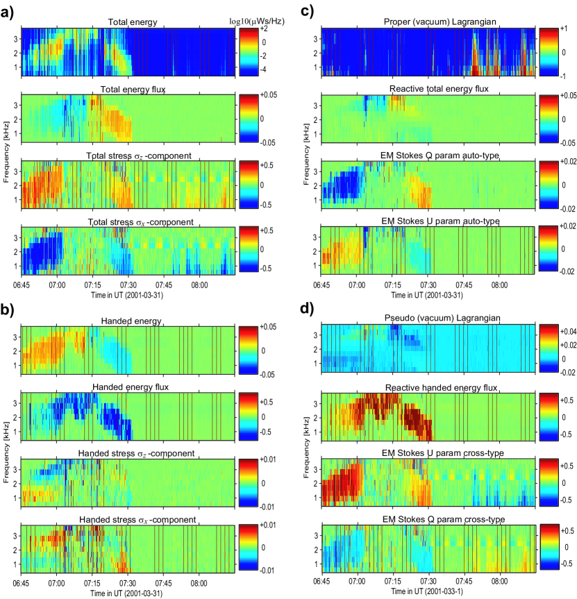
Figure 1: Example dynamic spectra of the 16 normalized two-dimensional CEO parameters. The parameters were computed from STAFF-SA data from Cluster space-craft 2 using the ISDAT database system. The following normalization has been applied: each parameter has been divided by the total energy except the total energy itself. Thus all spectral values are in dimensionless unit except for the total energy. This Figure can be compared with Fig. 1 in Parrot03a . The 16 parameters are subdivided into a) the total energy parameters, b) the handed energy parameters, c) the reactive total energy parameters, and d) the reactive handed energy parameters. Note that all the quantities are purely electromagnetic in origin and so do not refer to contributions from the plasma.

4 Application of CEO to Cluster data

Let us demonstrate that the CEO parameters can easily be computed from actual data. Assuming that we have measurements from a vector magnetometer and an electric field instrument, all that is required is to auto/cross-correlate all measured components and then form the appropriate linear combination introduced above.

As an example we will consider the STAFF-SA dataset on the Cluster-II space-craft mission Escoubet97 . The STAFF-SA instrument Cornilleau-Wehrlin1997 is well suited for the CEO parameters since it outputs auto/cross-correlation of electric and magnetic field components; however as Cluster does not measure one of the electric field components (namely the component normal to the spin-plane of the space-craft) we can only use the 2D version of the CEO introduced in the previous section.

For this particular example, we re-process the high-band part of STAFF-SA data from an event discussed in Parrot03a from 2001-03-31 UT. In Fig. 1 of this paper, Parrot et al display certain parameters based on the STAFF-SA data computed using a numerical software package called PRASSADCO; see Santolik2003 . The interesting feature of the 2D CEO parameters is that they are the complete set of electromagnetic field observables in the spin-plane of the space-craft; and indeed, they use up all the parameters in the STAFF-SA dataset expect for the magnetic field in the spin direction. Each CEO is a distinct physical quantity and examination of the panels in Fig. 1 indicates that this is indeed the case, since besides showing a common chorus feature (the arch to the left in each panel) there are unique points in each of the panels.

Besides being a complete description of the electromagnetic observables, the fact that the CEO parameters are based on parameters that conform with the physics of space-time means that we can expect physical phenomenon to be measured properly. Seeing as how the CEO parameters have not been explicitly measured in the past, we can expect that their future use may lead to new physical insights, especially since several of the parameters are completely new to space-physics. As an example consider again the data shown in Fig 1. It is interesting to note that the reactive total energy flux is only significant close to the equator; this implies that the equator is the source region for the chorus events, since reactive energy flux is typically large close to radiating objects due to large standing energy fields. One can also see a modulation at $2.5$ kHz in the EM Stokes parameters. If this is a physical phenomenon it would be indicative of Faraday rotation. Also there seems to be frequency dispersion in the handed stress since its components changes sign with frequency. Finally, the handed energy clearly shows the handedness of the chorus emissions on its own, without recourse to the sign of the total energy flux.

5 Conclusion

The proposed CEO parameters conveniently organize the measurements of the full EM field. Furthermore, they are physically meaningful quantities, i.e. they

• have conservation laws

• transform as geometric (Minkowski space-time) objects

• are mathematically unique (they are irreducible tensors)

• retain all information, i.e. nothing is lost (linear transformation back to full sixtor form exists)

• enables considerable data reduction (through parameter subset selection)

• have clear despinning properties (e.g. scalar quantities do not need despinning!)

• are all real valued

• provides useful decomposition of the 36 second order EM components into twelve 3-tensor quantities

• reveals some new physical parameters describing EM waves: opening for new physical insights.

References

- (1) L. R. O. Storey and F. Lefeuvre. Theory for the interpretations of measurements of the six components of a random electromagnetic wave field in space. Space Research, 14:381–386, 1974.
- (2) T. D. Carozzi and J. E. S. Bergman. Real irreducible sequilinear-quadratic tensor concomitants of complex bivectors. J. Math. Phys., 47:032903, 2006.
- (3) E. Wolf. Optics in terms of observable quantities. Il Nuovo Cimento, 12(6):884–888, December 1954.
- (4) A. O. Barut. Electrodynamics and Classical Theory of Fields and Particles. Dover, 1980.
- (5) D. Sundkvist. Covariant irreducible parameterization of electromagnetic fields in arbitrary space-time. J. Math. Phys., 47:012901, 2006.
- (6) S. Weinberg. Gravitation and Cosmology: Principles and Applications of the General Theory of Relativity. Wiley, New York, 1972.
- (7) Lenoid Lebedev and Michael J. Cloud. Tensor analysis. World Scientific, 2003.
- (8) M. Parrot, O. Santolík, N. Cornilleau-Wehrlin, M. Maksimovic, and C. C. Harvey. Source location of chorus emissions observed by cluster. Ann. Geophys., 21:473–480, 2003.
- (9) C.P. Escoubet, R. Schmidt, and C.T. Russell, editors. The Cluster and Phoenix Missions. Springer, 1997.
- (10) N. Cornilleau-Wehrlin et al. The Cluster Spatio-Temporal Analysis of Field Fluctuations (STAFF) Experiment’. Space Sci. Rev., 79(1–2):107–136, 1997.
- (11) Ondřej Santolík. Propagation analysis of STAFF-SA data with coherency tests (a user’s guide to PRASSADCO). Technical Report LPCE/NTS/073.D, LPCE/CNSR, 2003.