Water waves generated by a moving bottom

Abstract

Tsunamis are often generated by a moving sea bottom. This paper deals with the case where the tsunami source is an earthquake. The linearized water-wave equations are solved analytically for various sea bottom motions. Numerical results based on the analytical solutions are shown for the free-surface profiles, the horizontal and vertical velocities as well as the bottom pressure.

1 Introduction

Waves at the surface of a liquid can be generated by various mechanisms: wind blowing on the free surface, wavemaker, moving disturbance on the bottom or the surface, or even inside the liquid, fall of an object into the liquid, liquid inside a moving container, etc. In this paper, we concentrate on the case where the waves are created by a given motion of the bottom. One example is the generation of tsunamis by a sudden seafloor deformation.

There are different natural phenomena that can lead to a tsunami. For example, one can mention submarine slumps, slides, volcanic explosions, etc. In this article we use a submarine faulting generation mechanism as tsunami source. The resulting waves have some well-known features. For example, characteristic wavelengths are large and wave amplitudes are small compared with water depth.

Two factors are usually necessary for an accurate modelling of tsunamis: information on the magnitude and distribution of the displacements caused by the earthquake, and a model of surface gravity waves generation resulting from this motion of the seafloor. Most studies of tsunami generation assume that the initial free-surface deformation is equal to the vertical displacement of the ocean bottom. The details of wave motion are neglected during the time that the source operates. While this is often justified because the earthquake rupture occurs very rapidly, there are some specific cases where the time scale of the bottom deformation may become an important factor. This was emphasized for example by Trifunac and Todorovska [1], who considered the generation of tsunamis by a slowly spreading uplift of the seafloor and were able to explain some observations. During the 26 December 2004 Sumatra-Andaman event, there was in the northern extent of the source a relatively slow faulting motion that led to significant vertical bottom motion but left little record in the seismic data. It is interesting to point out that it is the inversion of tide-gauge data from Paradip, the northernmost of the Indian east-coast stations, that led Neetu et al. [2] to conclude that the source length was greater by roughly $30\%$ than the initial estimate of Lay et al. [3]. Incidentally, the generation time is also longer for landslide tsunamis.

Our study is restricted to the water region where the incompressible Euler equations for potential flow can be linearized. The wave propagation away from the source can be investigated by shallow water models which may or may not take into account nonlinear effects and frequency dispersion. Such models include the Korteweg-de Vries equation [4] for unidirectional propagation, nonlinear shallow-water equations and Boussinesq-type models [5, 6, 7].

Several authors have modeled the incompressible fluid layer as a special case of an elastic medium [8, 9, 10, 11, 12]. In our opinion it may be convenient to model the liquid by an elastic material from a mathematical point of view, but it is questionable from a physical point of view. The crust was modeled as an elastic isotropic half-space. This assumption will also be adopted in the present study.

The problem of tsunami generation has been considered by a number of authors: see for example [13, 14, 15]. The models discussed in these papers lack flexibility in terms of modelling the source due to the earthquake. The present paper provides some extensions. A good review on the subject is [16].

Here we essentially follow the framework proposed by Hammack [17] and others. The tsunami generation problem is reduced to a Cauchy-Poisson boundary value problem in a region of constant depth. The main extensions given in the present paper consist in three-dimensional modelling and more realistic source models. This approach was followed recently in [1, 18], where the mathematical model was the same as in [17] but the source was different.

Most analytical studies of linearized wave motion use integral transform methods. The complexity of the integral solutions forced many authors [9, 19] to use asymptotic methods such as the method of stationary phase to estimate the far-field behaviour of the solutions. In the present study we have also obtained asymptotic formulas for integral solutions. They are useful from a qualitative point of view, but in practice it is better to use numerical integration formulas [20] that take into account the oscillatory nature of the integrals. All the numerical results presented in this paper were obtained in this manner.

One should use asymptotic solutions with caution since they approximate exact solutions of the linearized problem. The relative importance of linear and nonlinear effects can be measured by the Stokes (or Ursell) number [21]:

$$U:=\frac{a/h}{(kh)^{2}}=\frac{a}{k^{2}h^{3}},$$

where $k$ is a wave number, $a$ a typical wave amplitude and $h$ the water depth. For $U\gg 1$, the nonlinear effects control wave propagation and only nonlinear models are applicable. Ursell [21] proved that near the wave front $U$ behaves like

$$U\sim t^{\frac{1}{3}}.$$

Hence, regardless of how small nonlinear effects are initially, they will become important.

Section 2 provides a description of the tsunami source when the source is an earthquake. In Section 3, we review the water-wave equations and provide the analytical solution to the linearized problem in the fluid domain. Section 4 is devoted to numerical results based on the analytical solution.

2 Source model

The inversion of seismic wave data allows the reconstruction of permanent deformations of the sea bottom following earthquakes. In spite of the complexity of the seismic source and of the internal structure of the earth, scientists have been relatively successful in using simple models for the source. One of these models is Okada’s model [22]. Its description follows.

The fracture zones, along which the foci of earthquakes are to be found, have been described in various papers. For example, it has been suggested that Volterra’s theory of dislocations might be the proper tool for a quantitative description of these fracture zones [23]. This suggestion was made for the following reason. If the mechanism involved in earthquakes and the fracture zones is indeed one of fracture, discontinuities in the displacement components across the fractured surface will exist. As dislocation theory may be described as that part of the theory of elasticity dealing with surfaces across which the displacement field is discontinuous, the suggestion makes sense.

As is often done in mathematical physics, it is necessary for simplicity’s sake to make some assumptions. Here we neglect the curvature of the earth, its gravity, temperature, magnetism, non-homogeneity, and consider a semi-infinite medium, which is homogeneous and isotropic. We further assume that the laws of classical linear elasticity theory hold.

Several studies showed that the effect of earth curvature is negligible for shallow events at distances of less than $20^{\circ}$ [24, 25, 26]. The sensitivity to earth topography, homogeneity, isotropy and half-space assumptions was studied and discussed recently [27]. A commercially available code, ABACUS, which is based on a finite element model (FEM), was used. Six FEMs were constructed to test the sensitivity of deformation predictions to each assumption. The author came to the conclusion that the vertical layering of lateral inhomogeneity can sometimes cause considerable effects on the deformation fields.

The usual boundary conditions for dealing with earth problems require that the surface of the elastic medium (the earth) shall be free from forces. The resulting mixed boundary-value problem was solved a century ago [28]. Later, Steketee proposed an alternative method to solve this problem using Green’s functions [23].

2.1 Volterra’s theory of dislocations

In order to introduce the concept of dislocation and for simplicity’s sake, this section is devoted to the case of an entire elastic space, as was done in the original paper by Volterra [28].

Let $O$ be the origin of a Cartesian coordinate system in an infinite elastic medium, $x_{i}$ the Cartesian coordinates $(i=1,2,3)$, and $\mathbf{e}_{i}$ a unit vector in the positive $x_{i}-$direction. A force $\mathbf{F}=F\mathbf{e}_{k}$ at $O$ generates a displacement field $u_{i}^{k}(P,O)$ at point $P$, which is determined by the well-known Somigliana tensor

$$u_{i}^{k}(P,O)=\frac{F}{8\pi\mu}(\delta_{ik}r_{,\>nn}-\alpha r_{,\>ik}),\quad\mbox{with}\;\;\alpha=\frac{\lambda+\mu}{\lambda+2\mu}.$$ (1)

In this relation $\delta_{ik}$ is the Kronecker delta, $\lambda$ and $\mu$ are Lamé’s constants, and $r$ is the distance from $P$ to $O$. The coefficient $\alpha$ can be rewritten as $\alpha=1/2(1-\nu)$, where $\nu$ is Poisson’s ratio. Later we will also use Young’s modulus $E$, which is defined as

$$E=\frac{\mu\,(3\lambda+2\mu)}{\lambda+\mu}.$$

The notation $r_{,\>i}$ means $\partial r/\partial x_{i}$ and the summation convention applies.

The stresses due to the displacement field (1) are easily computed from Hooke’s law:

$$\sigma_{ij}=\lambda\delta_{ij}u_{k,k}+\mu(u_{i,j}+u_{j,i}).$$ (2)

One finds

$$\sigma_{ij}^{k}(P,O)=-\frac{\alpha F}{4\pi}\left(\frac{3x_{i}x_{j}x_{k}}{r^{5}}+\frac{\mu}{\lambda+\mu}\frac{\delta_{ki}x_{j}+\delta_{kj}x_{i}-\delta_{ij}x_{k}}{r^{3}}\right).$$

The components of the force per unit area on a surface element are denoted as follows:

$$T_{i}^{k}=\sigma_{ij}^{k}\nu_{j},$$

where the $\nu_{j}$’s are the components of the normal to the surface element. A Volterra dislocation is defined as a surface $\Sigma$ in the elastic medium across which there is a discontinuity $\Delta u_{i}$ in the displacement fields of the type

$$\Delta u_{i} = u_{i}^{+}-u_{i}^{-}=U_{i}+\Omega_{ij}x_{j},$$ (3)

$$\Omega_{ij} = -\Omega_{ji}.$$ (4)

Equation (3) in which $U_{i}$ and $\Omega_{ij}$ are constants is the well-known Weingarten relation which states that the discontinuity $\Delta u_{i}$ should be of the type of a rigid body displacement, thereby maintaining continuity of the components of stress and strain across $\Sigma$.

The displacement field in an infinite elastic medium due to the dislocation is then determined by Volterra’s formula [28]

$$u_{k}(Q)=\frac{1}{F}\int\!\!\!\!\int\limits_{\!\!\!\!\!\!\!\Sigma}\Delta u_{i}T_{i}^{k}\,dS.$$ (5)

Once the surface $\Sigma$ is given, the dislocation is essentially determined by the six constants $U_{i}$ and $\Omega_{ij}$. Therefore we also write

$$u_{k}(Q)=\frac{U_{i}}{F}\int\!\!\!\!\int\limits_{\!\!\!\!\!\!\!\Sigma}\sigma_{ij}^{k}(P,Q)\nu_{j}dS+\frac{\Omega_{ij}}{F}\int\!\!\!\!\int\limits_{\!\!\!\!\!\!\!\Sigma}\{x_{j}\sigma_{il}^{k}(P,Q)-x_{i}\sigma_{jl}^{k}(P,Q)\}\nu_{l}dS,$$ (6)

where $\Omega_{ij}$ takes only the values $\Omega_{12}$, $\Omega_{23}$, $\Omega_{31}$. Following Volterra [28] and Love [29] we call each of the six integrals in (6) an elementary dislocation.

It is clear from (5) and (6) that the computation of the displacement field $u_{k}(Q)$ is performed as follows. A force $F\mathbf{e}_{k}$ is applied at $Q$, and the stresses $\sigma_{ij}^{k}(P,Q)$ that this force generates are computed at the points $P(x_{i})$ on $\Sigma$. In particular the components of the force on $\Sigma$ are computed. After multiplication with prescribed weights of magnitude $\Delta u_{i}$ these forces are integrated over $\Sigma$ to give the displacement component in $Q$ due to the dislocation on $\Sigma$.

2.2 Dislocations in elastic half-space

When the case of an elastic half-space is considered, equation (5) remains valid, but we have to replace $\sigma_{ij}^{k}$ in $T_{i}^{k}$ by another tensor $\omega_{ij}^{k}$. This can be explained by the fact that the elementary solutions for a half-space are different from Somigliana solution (1).

The $\omega_{ij}^{k}$ can be obtained from the displacements corresponding to nuclei of strain in a half-space through relation (2). Steketee showed a method of obtaining the six $\omega_{ij}^{k}$ fields by using a Green’s function and derived $\omega_{12}^{k}$, which is relevant to a vertical strike-slip fault (see below). Maruyama derived the remaining five functions [30].

It is interesting to mention here that historically these solutions were first derived in a straightforward manner by Mindlin [31, 32], who gave explicit expressions of the displacement and stress fields for half-space nuclei of strain consisting of single forces with and without moment. It is only necessary to write the single force results since the other forms can be obtained by taking appropriate derivatives. The method consists in finding the displacement field in Westergaard’s form of the Galerkin vector [33]. This vector is then determined by taking a linear combination of some biharmonic elementary solutions. The coefficients are chosen to satisfy boundary and equilibrium conditions. These solutions were also derived by Press in a slightly different manner [34].

Figure 1: Coordinate system adopted in this study and geometry of the source model

Here, we take the Cartesian coordinate system shown in Figure 1. The elastic medium occupies the region $x_{3}\leq 0$ and the $x_{1}-$axis is taken to be parallel to the strike direction of the fault. In this coordinate system, $u_{i}^{j}(x_{1},x_{2},x_{3};\xi_{1},\xi_{2},\xi_{3})$ is the $i$th component of the displacement at $(x_{1},x_{2},x_{3})$ due to the $j$th direction point force of magnitude $F$ at $(\xi_{1},\xi_{2},\xi_{3})$. It can be expressed as follows [22, 31, 34, 35]:

$$u_{i}^{j}(x_{1},x_{2},x_{3}) = u_{iA}^{j}(x_{1},x_{2},-x_{3})-u_{iA}^{j}(x_{1},x_{2},x_{3})$$

$$+u_{iB}^{j}(x_{1},x_{2},x_{3})+x_{3}u_{iC}^{j}(x_{1},x_{2},x_{3}),$$

where

$$u_{iA}^{j} = \frac{F}{8\pi\mu}\left((2-\alpha)\frac{\delta_{ij}}{R}+\alpha\frac{R_{i}R_{j}}{R^{3}}\right),$$

$$u_{iB}^{j} = \frac{F}{4\pi\mu}\Biggl{(}\frac{\delta_{ij}}{R}+\frac{R_{i}R_{j}}{R^{3}}+\frac{1-\alpha}{\alpha}\Bigl{[}\frac{\delta_{ij}}{R+R_{3}}+$$

$$+\frac{R_{i}\delta_{j3}-R_{j}\delta_{i3}(1-\delta_{j3})}{R(R+R_{3})}-\frac{R_{i}R_{j}}{R(R+R_{3})^{2}}(1-\delta_{i3})(1-\delta_{j3})\Bigr{]}\Biggr{)},$$

$$u_{iC}^{j} = \frac{F}{4\pi\mu}(1-2\delta_{i3})\left((2-\alpha)\frac{R_{i}\delta_{j3}-R_{j}\delta_{i3}}{R^{3}}+\alpha\xi_{3}\left[\frac{\delta_{ij}}{R^{3}}-3\frac{R_{i}R_{j}}{R^{5}}\right]\right).$$

In these expressions $R_{1}=x_{1}-\xi_{1}$, $R_{2}=x_{2}-\xi_{2}$, $R_{3}=-x_{3}-\xi_{3}$ and $R^{2}=R_{1}^{2}+R_{2}^{2}+R_{3}^{2}$.

The first term in equation (2.2), $u_{iA}^{j}(x_{1},x_{2},-x_{3})$, is the well-known Somigliana tensor, which represents the displacement field due to a single force placed at $(\xi_{1},\xi_{2},\xi_{3})$ in an infinite medium [29]. The second term also looks like a Somigliana tensor. This term corresponds to a contribution from an image source of the given point force placed at $(\xi_{1},\xi_{2},-\xi_{3})$ in the infinite medium. The third term, $u_{iB}^{j}(x_{1},x_{2},x_{3})$, and $u_{iC}^{j}(x_{1},x_{2},x_{3})$ in the fourth term are naturally depth dependent. When $x_{3}$ is set equal to zero in equation (2.2), the first and the second terms cancel each other, and the fourth term vanishes. The remaining term, $u_{iB}^{j}(x_{1},x_{2},0)$, reduces to the formula for the surface displacement field due to a point force in a half-space [22]:

$$\left\{\begin{array}[]{ll}u_{1}^{1}=\frac{F}{4\pi\mu}\left(\frac{1}{R}+\frac{(x_{1}-\xi_{1})^{2}}{R^{3}}+\frac{\mu}{\lambda+\mu}\left[\frac{1}{R-\xi_{3}}-\frac{(x_{1}-\xi_{1})^{2}}{R(R-\xi_{3})^{2}}\right]\right),&\\ u_{2}^{1}=\frac{F}{4\pi\mu}(x_{1}-\xi_{1})(x_{2}-\xi_{2})\left(\frac{1}{R^{3}}-\frac{\mu}{\lambda+\mu}\frac{1}{R(R-\xi_{3})^{2}}\right),&\\ u_{3}^{1}=\frac{F}{4\pi\mu}(x_{1}-\xi_{1})\left(-\frac{\xi_{3}}{R^{3}}-\frac{\mu}{\lambda+\mu}\frac{1}{R(R-\xi_{3})}\right),&\end{array}\right.$$

$$\left\{\begin{array}[]{ll}u_{1}^{2}=\frac{F}{4\pi\mu}(x_{1}-\xi_{1})(x_{2}-\xi_{2})\left(\frac{1}{R^{3}}-\frac{\mu}{\lambda+\mu}\frac{1}{R(R-\xi_{3})^{2}}\right),&\\ u_{2}^{2}=\frac{F}{4\pi\mu}\left(\frac{1}{R}+\frac{(x_{2}-\xi_{2})^{2}}{R^{3}}+\frac{\mu}{\lambda+\mu}\left[\frac{1}{R-\xi_{3}}-\frac{(x_{2}-\xi_{2})^{2}}{R(R-\xi_{3})^{2}}\right]\right),&\\ u_{3}^{2}=\frac{F}{4\pi\mu}(x_{2}-\xi_{2})\left(-\frac{\xi_{3}}{R^{3}}-\frac{\mu}{\lambda+\mu}\frac{1}{R(R-\xi_{3})}\right),&\end{array}\right.$$

$$\left\{\begin{array}[]{ll}u_{1}^{3}=\frac{F}{4\pi\mu}(x_{1}-\xi_{1})\left(-\frac{\xi_{3}}{R^{3}}+\frac{\mu}{\lambda+\mu}\frac{1}{R(R-\xi_{3})}\right),&\\ u_{2}^{3}=\frac{F}{4\pi\mu}(x_{2}-\xi_{2})\left(-\frac{\xi_{3}}{R^{3}}+\frac{\mu}{\lambda+\mu}\frac{1}{R(R-\xi_{3})}\right),&\\ u_{3}^{3}=\frac{F}{4\pi\mu}\left(\frac{1}{R}+\frac{\xi_{3}^{2}}{R^{3}}+\frac{\mu}{\lambda+\mu}\frac{1}{R}\right).&\end{array}\right.$$

In these formulas $R^{2}=(x_{1}-\xi_{1})^{2}+(x_{2}-\xi_{2})^{2}+\xi_{3}^{2}$.

In order to obtain the displacements due to the dislocation we need to calculate the corresponding $\xi_{k}$-derivatives of the point force solution (2.2) and to insert them in Volterra’s formula (5)

$$u_{i}=\frac{1}{F}\int\!\!\!\!\int\limits_{\!\!\!\!\!\!\!\Sigma}\Delta u_{j}\left[\lambda\delta_{jk}\frac{\partial u_{i}^{n}}{\partial\xi_{n}}+\mu\left(\frac{\partial u_{i}^{j}}{\partial\xi_{k}}+\frac{\partial u_{i}^{k}}{\partial\xi_{j}}\right)\right]\nu_{k}\,dS.$$

The $\xi_{k}$-derivatives are expressed as follows:

$$\frac{\partial u_{i}^{j}}{\partial\xi_{k}}(x_{1},x_{2},x_{3}) = \frac{\partial u_{iA}^{j}}{\partial\xi_{k}}(x_{1},x_{2},-x_{3})-\frac{\partial u_{iA}^{j}}{\partial\xi_{k}}(x_{1},x_{2},x_{3})+$$

$$+\frac{\partial u_{iB}^{j}}{\partial\xi_{k}}(x_{1},x_{2},x_{3})+x_{3}\frac{\partial u_{iC}^{j}}{\partial\xi_{k}}(x_{1},x_{2},x_{3}),$$

with

$$\frac{\partial u_{iA}^{j}}{\partial\xi_{k}} = \frac{F}{8\pi\mu}\left((2-\alpha)\frac{R_{k}}{R^{3}}\delta_{ij}-\alpha\frac{R_{i}\delta_{jk}+R_{j}\delta_{ik}}{R^{3}}+3\alpha\frac{R_{i}R_{j}R_{k}}{R^{5}}\right),$$

$$\frac{\partial u_{iB}^{j}}{\partial\xi_{k}} = \frac{F}{4\pi\mu}\left(-\frac{R_{i}\delta_{jk}+R_{j}\delta_{ik}-R_{k}\delta_{ij}}{R^{3}}+3\frac{R_{i}R_{j}R_{k}}{R^{5}}\right.+$$

$$+\frac{1-\alpha}{\alpha}\Bigl{[}\frac{\delta_{3k}R+R_{k}}{R(R+R_{3})^{2}}\delta_{ij}-\frac{\delta_{ik}\delta_{j3}-\delta_{jk}\delta_{i3}(1-\delta_{j3})}{R(R+R_{3})}+$$

$$+\bigl{(}R_{i}\delta_{j3}-R_{j}\delta_{i3}(1-\delta_{j3})\bigr{)}\frac{\delta_{3k}R^{2}+R_{k}(2R+R_{3})}{R^{3}(R+R_{3})^{2}}+$$

$$\left.+(1-\delta_{i3})(1-\delta_{j3})\bigl{(}\frac{R_{i}\delta_{jk}+R_{j}\delta_{ik}}{R(R+R_{3})^{2}}-R_{i}R_{j}\frac{2\delta_{3k}R^{2}+R_{k}(3R+R_{3})}{R^{3}(R+R_{3})^{3}}\bigr{)}\Bigr{]}\right),$$

$$\frac{\partial u_{iC}^{j}}{\partial\xi_{k}} = \frac{F}{4\pi\mu}(1-2\delta_{i3})\biggl{(}(2-\alpha)\Bigl{[}\frac{\delta_{jk}\delta_{i3}-\delta_{ik}\delta_{j3}}{R^{3}}+\frac{3R_{k}(R_{i}\delta_{j3}-R_{j}\delta_{i3})}{R^{5}}\Bigr{]}+$$

$$+\alpha\delta_{3k}\Bigl{[}\frac{\delta_{ij}}{R^{3}}-\frac{3R_{i}R_{j}}{R^{5}}\Bigr{]}+3\alpha\xi_{3}\Bigl{[}\frac{R_{i}\delta_{jk}+R_{j}\delta_{ik}+R_{k}\delta_{ij}}{R^{5}}-\frac{5R_{i}R_{j}R_{k}}{R^{7}}\Bigr{]}\biggr{)}.$$

2.3 Finite rectangular source

Let us now consider a more practical problem. We define the elementary dislocations $U_{1}$, $U_{2}$ and $U_{3}$, corresponding to the strike-slip, dip-slip and tensile components of an arbitrary dislocation. In Figure 1 each vector represents the direction of the elementary faults. The vector $\mathbf{D}$ is the so-called Burger’s vector, which shows how both sides of the fault are spread out: $\mathbf{D}=\mathbf{u}^{+}-\mathbf{u}^{-}$.

A general dislocation can be determined by three angles: the dip angle $\delta$ of the fault $(0\leq\delta\leq\pi)$, the slip or rake angle $\theta$ $(0\leq\theta\leq\pi)$, and the angle $\phi$ between the fault plane and Burger’s vector $\mathbf{D}$. When dealing with a geophysical application, an additional angle, the azimuth or strike, is introduced in order to provide an orientation of the fault. The general situation is schematically described in Figure 2.

Figure 2: Geometry of the source model and orientation of Burger’s vector $\mathbf{D}$

For a finite rectangular fault with length $L$ and width $W$ occurring at depth $d$ (Figure 2), the deformation field can be evaluated analytically by a change of variables and by integrating over the rectangle. This was done by several authors [22, 35, 36, 37, 38]. Here we give the results of their computations. The final results are represented below in compact form, using Chinnery’s notation $\|$ to represent the substitution

$$f(\xi,\eta)\|=f(x,p)-f(x,p-W)-f(x-L,p)+f(x-L,p-W),$$

where $p=y\cos\delta+d\sin\delta$. Next we introduce the notation

$$q=y\sin\delta-d\cos\delta,\quad\tilde{y}=\eta\cos\delta+q\sin\delta,\quad\tilde{d}=\eta\sin\delta-q\cos\delta$$

and

$$R^{2}=\xi^{2}+\eta^{2}+q^{2}=\xi^{2}+\tilde{y}^{2}+\tilde{d}^{2},\quad X^{2}=\xi^{2}+q^{2}.$$

The quantities $U_{1}$, $U_{2}$ and $U_{3}$ are linked to Burger’s vector through the identities

$$U_{1}=|\mathbf{D}|\cos\phi\cos\theta,\quad U_{2}=|\mathbf{D}|\cos\phi\sin\theta,\quad U_{3}=|\mathbf{D}|\sin\phi.$$

For a strike-slip dislocation, one has

$$u_{1} = -\frac{U_{1}}{2\pi}\left.\left(\frac{\xi q}{R(R+\eta)}+\arctan\frac{\xi\eta}{qR}+I_{1}\sin\delta\right)\right\|,$$

$$u_{2} = -\frac{U_{1}}{2\pi}\left.\left(\frac{\tilde{y}q}{R(R+\eta)}+\frac{q\cos\delta}{R+\eta}+I_{2}\sin\delta\right)\right\|,$$

$$u_{3} = -\frac{U_{1}}{2\pi}\left.\left(\frac{\tilde{d}q}{R(R+\eta)}+\frac{q\sin\delta}{R+\eta}+I_{4}\sin\delta\right)\right\|.$$

For a dip-slip dislocation, one has

$$u_{1} = -\frac{U_{2}}{2\pi}\left.\left(\frac{q}{R}-I_{3}\sin\delta\cos\delta\right)\right\|,$$

$$u_{2} = -\frac{U_{2}}{2\pi}\left.\left(\frac{\tilde{y}q}{R(R+\xi)}+\cos\delta\arctan\frac{\xi\eta}{qR}-I_{1}\sin\delta\cos\delta\right)\right\|,$$

$$u_{3} = -\frac{U_{2}}{2\pi}\left.\left(\frac{\tilde{d}q}{R(R+\xi)}+\sin\delta\arctan\frac{\xi\eta}{qR}-I_{5}\sin\delta\cos\delta\right)\right\|.$$

For a tensile fault dislocation, one has

$$u_{1} = \frac{U_{3}}{2\pi}\left.\left(\frac{q^{2}}{R(R+\eta)}-I_{3}\sin^{2}\delta\right)\right\|,$$

$$u_{2} = \frac{U_{3}}{2\pi}\left.\left(\frac{-\tilde{d}q}{R(R+\xi)}-\sin\delta\left[\frac{\xi q}{R(R+\eta)}-\arctan\frac{\xi\eta}{qR}\right]-I_{1}\sin^{2}\delta\right)\right\|,$$

$$u_{3} = \frac{U_{3}}{2\pi}\left.\left(\frac{\tilde{y}q}{R(R+\xi)}+\cos\delta\left[\frac{\xi q}{R(R+\eta)}-\arctan\frac{\xi\eta}{qR}\right]-I_{5}\sin^{2}\delta\right)\right\|.$$

The terms $I_{1},\dots,I_{5}$ are given by

$$I_{1} = -\frac{\mu}{\lambda+\mu}\frac{\xi}{(R+\tilde{d})\cos\delta}-\tan\delta I_{5},$$

$$I_{2} = -\frac{\mu}{\lambda+\mu}\log(R+\eta)-I_{3},$$

$$I_{3} = \frac{\mu}{\lambda+\mu}\left[\frac{1}{\cos\delta}\frac{\tilde{y}}{R+\tilde{d}}-\log(R+\eta)\right]+\tan\delta I_{4},$$

$$I_{4} = \frac{\mu}{\mu+\lambda}\frac{1}{\cos\delta}\left(\log(R+\tilde{d})-\sin\delta\log(R+\eta)\right),$$

$$I_{5} = \frac{\mu}{\lambda+\mu}\frac{2}{\cos\delta}\arctan\frac{\eta(X+q\cos\delta)+X(R+X)\sin\delta}{\xi(R+X)\cos\delta},$$

and if $\cos\delta=0$,

$$I_{1} = -\frac{\mu}{2(\lambda+\mu)}\frac{\xi q}{(R+\tilde{d})^{2}},$$

$$I_{3} = \frac{\mu}{2(\lambda+\mu)}\left[\frac{\eta}{R+\tilde{d}}+\frac{\tilde{y}q}{(R+\tilde{d})^{2}}-\log(R+\eta)\right],$$

$$I_{4} = -\frac{\mu}{\lambda+\mu}\frac{q}{R+\tilde{d}},$$

$$I_{5} = -\frac{\mu}{\lambda+\mu}\frac{\xi\sin\delta}{R+\tilde{d}}.$$

Figures 3, 4, and 5 show the free-surface deformation due to the three elementary dislocations. The values of the parameters are given in Table 1.

parameter	value
Dip angle $\delta$	$13^{\circ}$
Fault depth $d$, km	25
Fault length $L$, km	220
Fault width $W$, km	90
$U_{i}$, m	15
Young modulus $E$, GPa	9.5
Poisson’s ratio $\nu$	0.23

Table 1: Parameter set used in Figures 3, 4, and 5.

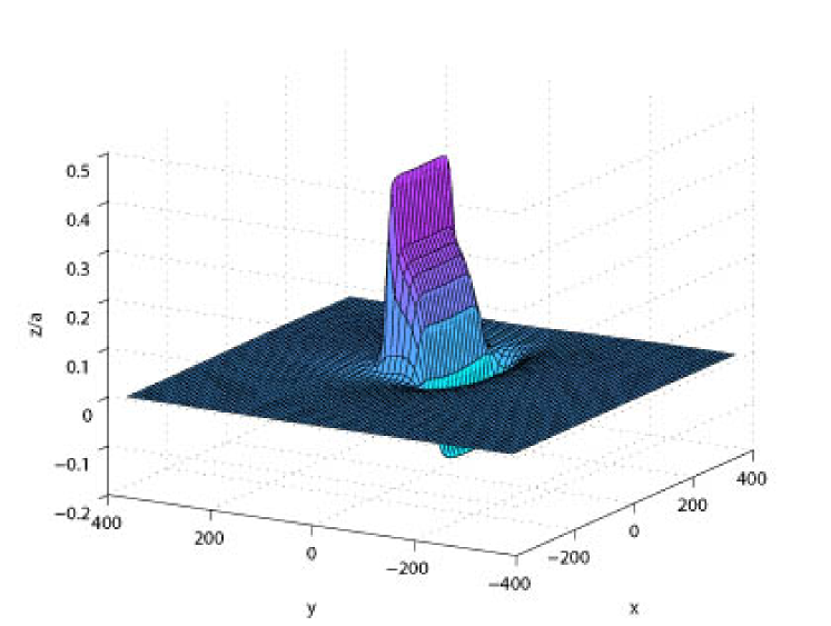
Figure 3: Dimensionless free-surface deformation $z/a$ due to dip-slip faulting: $\phi=0$, $\theta=\pi/2$, $\mathbf{D}=(0,U_{2},0)$. Here $a$ is $|\mathbf{D}|$ (15 m in the present application). The horizontal distances $x$ and $y$ are expressed in kilometers.

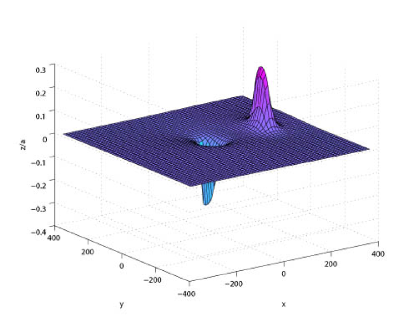
Figure 4: Dimensionless free-surface deformation $z/a$ due to strike-slip faulting: $\phi=0$, $\theta=0$, $\mathbf{D}=(U_{1},0,0)$. Here $a$ is $|\mathbf{D}|$ (15 m in the present application). The horizontal distances $x$ and $y$ are expressed in kilometers.

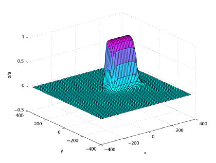
Figure 5: Dimensionless free-surface deformation $z/a$ due to tensile faulting: $\phi=\pi/2$, $\mathbf{D}=(0,0,U_{3})$. Here $a$ is $|\mathbf{D}|$. The horizontal distances $x$ and $y$ are expressed in kilometers.

2.4 Curvilinear fault

In the previous subsection analytical formulas for the free-surface deformation in the special case of a rectangular fault were given. In fact, Volterra’s formula (5) allows to evaluate the displacement field that accompanies fault events with much more general geometry. The shape of the fault and Burger’s vector are suggested by seismologists and after numerical integration one can obtain the deformation of the seafloor for more general types of events as well.

Here we will consider the case of a fault whose geometry is described by an elliptical arc (see Figure 6).

Figure 6: Geometry of a fault with elliptical shape.

The parametric equations of this surface are given by

$$x(\xi,\eta)=\xi,\quad 0\leq\xi\leq a,\qquad y(\xi,\eta)=\eta,\quad-\frac{c}{2}\leq\eta\leq\frac{c}{2},$$

$$z(\xi,\eta)=-(b+d)+\frac{b}{a}\sqrt{a^{2}-\xi^{2}}.$$

Then the unit normal to this surface can be easily calculated:

$$\mathbf{n}=\left(\frac{b\xi}{\sqrt{a^{4}+(b^{2}-a^{2})\xi^{2}}},0,\frac{a\sqrt{a^{2}-\xi^{2}}}{\sqrt{a^{4}+(b^{2}-a^{2})\xi^{2}}}\right).$$

We also need to compute the coefficients of the first fundamental form in order to reduce the surface integral in (5) to a double Riemann integral. These coefficients are

$$E=\frac{a^{4}+\xi^{2}(b^{2}-a^{2})}{a^{2}(a^{2}-\xi^{2})},\quad F=0,\quad G=1$$

and the surface element $dS$ is

$$dS=\sqrt{EG-F^{2}}\,d\xi d\eta=\frac{1}{a}\frac{\sqrt{a^{4}+\xi^{2}(b^{2}-a^{2})}}{\sqrt{a^{2}-\xi^{2}}}\,d\xi d\eta.$$

Since in the crust the hydrostatic pressure is very large, it is natural to impose the condition that $\mathbf{D}\cdot\mathbf{n}=0.$ The physical meaning of this condition is that both sides of the fault slide and do not detach. This condition is obviously satisfied if we take Burger’s vector as

$$\mathbf{D}=D\left(\frac{a\sqrt{a^{2}-\xi^{2}}}{\sqrt{a^{4}+\xi^{2}(b^{2}-a^{2})}},0,-\frac{b\xi}{\sqrt{a^{4}+\xi^{2}(b^{2}-a^{2})}}\right).$$

It is evident that $D=|\mathbf{D}|$.

The numerical integration was performed using a $9$-point two-dimensional Gauss-type integration formula. The result is presented on Figure 7. The parameter values are given in Table 2.

parameter	value
Depth event $d$, km	20
Ellipse semiminor axis $a$, km	17
Ellipse semimajor axis $b$, km	6
Fault width $c$, km	15
Young modulus $E$, GPa	9.5
Poisson’s ratio $\nu$	0.23

Table 2: Parameter set used in Figure 7.

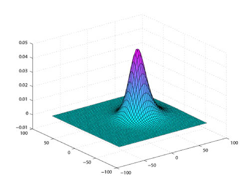
Figure 7: Free-surface deformation due to curvilinear faulting. The horizontal distances $x$ and $y$ are expressed in kilometers.

The example considered in this subsection may not be physically relevant. However it shows how Okada’s solution can be extended. For a more precise modeling of the faulting event we need to have more information about the earthquake source and its related parameters.

After having reviewed the description of the source, we now switch to the deformation of the ocean surface following a submarine earthquake. The traditional approach for hydrodynamic modelers is to use elastic models similar to the model we just described with the seismic parameters as input in order to evaluate the details of the seafloor deformation. Then this deformation is translated to the free surface of the ocean and serves as initial condition of the evolution problem described in the next section.

3 Solution in fluid domain

Figure 8: Definition of the fluid domain and coordinate system

The fluid domain is supposed to represent the ocean above the fault area. Let us consider the fluid domain $\Omega$ shown in Figure 8. It is bounded above by the free surface of the ocean and below by the rigid ocean floor. The domain $\Omega$ is unbounded in the horizontal directions $x$ and $y$, and can be written as

$$\Omega=\mathbb{R}^{2}\times\left[-h+\zeta(x,y,t),\eta(x,y,t)\right].$$

Initially the fluid is assumed to be at rest and the sea bottom to be horizontal. Thus, at time $t=0$, the free surface and the sea bottom are defined by $z=0$ and $z=-h$, respectively. For time $t>0$ the bottom boundary moves in a prescribed manner which is given by

$$z=-h+\zeta(x,y,t).$$

The displacement of the sea bottom is assumed to have all the properties required to compute its Fourier transform in $x,y$ and its Laplace transform in $t$. The resulting deformation of the free surface $z=\eta(x,y,t)$ must be found. It is also assumed that the fluid is incompressible and the flow is irrotational. The latter implies the existence of a velocity potential $\phi(x,y,z,t)$ which completely describes this flow. By definition of $\phi$, the fluid velocity vector can be expressed as $\mathbf{q}=\nabla\phi$. Thus, the continuity equation becomes

$$\nabla\cdot\mathbf{q}=\Delta\phi=0,\quad(x,y,z)\in\Omega.$$ (8)

The potential $\phi(x,y,z,t)$ must also satisfy the following kinematic boundary conditions on the free-surface and the solid boundary, respectively:

$$\frac{\partial\phi}{\partial z} = \frac{\partial\eta}{\partial t}+\frac{\partial\phi}{\partial x}\frac{\partial\eta}{\partial x}+\frac{\partial\phi}{\partial y}\frac{\partial\eta}{\partial y},\qquad z=\eta(x,y,t),$$ (9)

$$\frac{\partial\phi}{\partial z} = \frac{\partial\zeta}{\partial t}+\frac{\partial\phi}{\partial x}\frac{\partial\zeta}{\partial x}+\frac{\partial\phi}{\partial y}\frac{\partial\zeta}{\partial y},\qquad z=-h+\zeta(x,y,t).$$ (10)

Assuming that viscous effects as well as capillary effects can be neglected, the dynamic condition to be satisfied on the free surface reads

$$\frac{\partial\phi}{\partial t}+\frac{1}{2}|\nabla\phi|^{2}+g\eta=0,\qquad z=\eta(x,y,t).$$ (11)

As described above, the initial conditions are given by

$$\eta(x,y,0)=0\quad\mbox{and}\quad\zeta(x,y,0)=0.$$ (12)

The significance of the various terms in the equations is more transparent when the equations are written in dimensionless variables. The new independent variables are

$$\widetilde{x}=\kappa x,\quad\widetilde{y}=\kappa y,\quad\widetilde{z}=\kappa z,\quad\widetilde{t}=\sigma t,$$

where $\kappa$ is a wavenumber and $\sigma$ is a typical frequency. Note that here the same unit length is used in the horizontal and vertical directions, as opposed to shallow-water theory.

The new dependent variables are

$$\widetilde{\eta}=\frac{\eta}{a},\quad\widetilde{\zeta}=\frac{\zeta}{a},\quad\widetilde{\phi}=\frac{\kappa}{a\sigma}\phi,$$

where $a$ is a characteristic wave amplitude. A dimensionless water depth is also introduced:

$$\widetilde{h}=\kappa h.$$

In dimensionless form, and after dropping the tildes, equations (8–11) become

$$\Delta\phi=0,\qquad(x,y,z)\in\Omega,$$

$$\frac{\partial\phi}{\partial z} = \frac{\partial\eta}{\partial t}+\kappa a\left(\frac{\partial\phi}{\partial x}\frac{\partial\eta}{\partial x}+\frac{\partial\phi}{\partial y}\frac{\partial\eta}{\partial y}\right),\qquad z=\kappa a\,\eta(x,y,t),$$

$$\frac{\partial\phi}{\partial z} = \frac{\partial\zeta}{\partial t}+\kappa a\left(\frac{\partial\phi}{\partial x}\frac{\partial\zeta}{\partial x}+\frac{\partial\phi}{\partial y}\frac{\partial\zeta}{\partial y}\right),\qquad z=-h+\kappa a\,\zeta(x,y,t),$$

$$\frac{\partial\phi}{\partial t}+\frac{1}{2}\kappa a|\nabla\phi|^{2}+\frac{g\kappa}{\sigma^{2}}\eta=0,\qquad z=\kappa a\,\eta(x,y,t).$$

Finding the solution to this problem is quite a difficult task due to the nonlinearities and the a priori unknown free surface. In this study we linearize the equations and the boundary conditions by taking the limit as $\kappa a\to 0$. In fact, the linearized problem can be found by expanding the unknown functions as power series of a small parameter $\varepsilon:=\kappa a$. Collecting the lowest order terms in $\varepsilon$ yields the linear approximation. For the sake of convenience, we now switch back to the physical variables. The linearized problem in dimensional variables reads

$$\Delta\phi=0,\qquad(x,y,z)\in\mathbb{R}^{2}\times[-h,0],$$ (13)

$$\frac{\partial\phi}{\partial z}=\frac{\partial\eta}{\partial t},\qquad z=0,$$ (14)

$$\frac{\partial\phi}{\partial z}=\frac{\partial\zeta}{\partial t},\qquad z=-h,$$ (15)

$$\frac{\partial\phi}{\partial t}+g\eta=0,\qquad z=0.$$ (16)

Combining equations (14) and (16) yields the single free-surface condition

$$\frac{\partial^{2}\phi}{\partial t^{2}}+g\frac{\partial\phi}{\partial z}=0,\qquad z=0.$$ (17)

This problem will be solved by using the method of integral transforms. We apply the Fourier transform in $(x,y)$:

$$\mathfrak{F}[f] = \widehat{f}(k,\ell)=\int\limits_{\mathbb{R}^{2}}f(x,y)e^{-i(kx+\ell y)}\,dxdy,$$

$$\mathfrak{F}^{-1}[\widehat{f}] = f(x,y)=\frac{1}{(2\pi)^{2}}\int\limits_{\mathbb{R}^{2}}\widehat{f}(k,\ell)e^{i(kx+\ell y)}\,dkd\ell,$$

and the Laplace transform in time $t$:

$$\mathfrak{L}[g]=\mathrm{g}(s)=\int\limits_{0}^{+\infty}g(t)e^{-st}\,dt.$$

For the combined Fourier and Laplace transforms, the following notation is introduced:

$$\mathfrak{F}\mathfrak{L}[F(x,y,t)]=\overline{F}(k,\ell,s)=\int\limits_{\mathbb{R}^{2}}e^{-i(kx+\ell y)}\,dxdy\int\limits_{0}^{+\infty}F(x,y,t)e^{-st}\,dt.$$

After applying the transforms, equations (13), (15) and (17) become

$$\frac{d^{2}\overline{\phi}}{dz^{2}}-(k^{2}+\ell^{2})\overline{\phi}=0,$$ (18)

$$\frac{d\overline{\phi}}{dz}(k,\ell,-h,s)=s\overline{\zeta}(k,\ell,s),$$ (19)

$$s^{2}\overline{\phi}(k,\ell,0,s)+g\frac{d\overline{\phi}}{dz}(k,\ell,0,s)=0.$$ (20)

The transformed free-surface elevation can be obtained from (16):

$$\overline{\eta}(k,\ell,s)=-\frac{s}{g}\overline{\phi}(k,\ell,0,s).$$ (21)

A general solution of equation (18) is given by

$$\overline{\phi}(k,\ell,z,s)=A(k,\ell,s)\cosh(mz)+B(k,\ell,s)\sinh(mz),$$ (22)

where $m=\sqrt{k^{2}+\ell^{2}}$. The functions $A(k,\ell,s)$ and $B(k,\ell,s)$ can be easily found from the boundary conditions (19) and (20):

$$A(k,\ell,s) = -\frac{gs\overline{\zeta}(k,\ell,s)}{\cosh(mh)[s^{2}+gm\tanh(mh)]},$$

$$B(k,\ell,s) = \frac{s^{3}\overline{\zeta}(k,\ell,s)}{m\cosh(mh)[s^{2}+gm\tanh(mh)]}.$$

From now on, the notation

$$\omega=\sqrt{gm\tanh(mh)}$$ (23)

will be used. The graphs of $\omega(m)$, $\omega^{\prime}(m)$ and $\omega^{\prime\prime}(m)$ are shown in Figure 9.

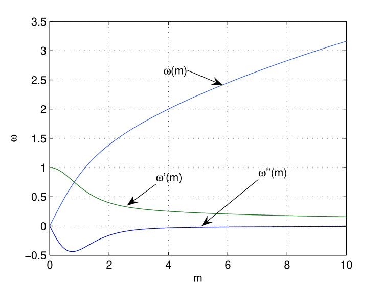
Figure 9: Plot of the frequency $\omega(m)=\sqrt{gm\tanh(mh)}$ and its derivatives $d\omega/dm$, $d^{2}\omega/dm^{2}$. The acceleration due to gravity $g$ and the water depth $h$ have been set equal to 1.

Substituting the expressions for the functions $A$, $B$ in (22) yields

$$\overline{\phi}(k,\ell,z,s)=-\frac{gs\overline{\zeta}(k,\ell,s)}{\cosh(mh)(s^{2}+\omega^{2})}\left(\cosh(mz)-\frac{s^{2}}{gm}\sinh(mz)\right).$$ (24)

3.1 Free-surface elevation

From (21), the free-surface elevation becomes

$$\overline{\eta}(k,\ell,s)=\frac{s^{2}\overline{\zeta}(k,\ell,s)}{\cosh(mh)(s^{2}+\omega^{2})}.$$

Inverting the Laplace and Fourier transforms provides the general integral solution

$$\eta(x,y,t)=\frac{1}{(2\pi)^{2}}\int\!\!\!\int\limits_{\!\!\!\!\!\mathbb{R}^{2}}\frac{e^{i(kx+\ell y)}}{\cosh(mh)}\frac{1}{2\pi i}\int\limits_{\mu-i\infty}^{\mu+i\infty}\frac{s^{2}\overline{\zeta}(k,\ell,s)}{s^{2}+\omega^{2}}e^{st}ds\;dkd\ell.$$ (25)

One can evaluate the Laplace integral in (25) using the convolution theorem:

$$\mathfrak{L}[f_{1}(t)*f_{2}(t)]=\mathrm{f_{1}}(s)\mathrm{f_{2}}(s).$$

It yields

$$\eta(x,y,t)=\frac{1}{(2\pi)^{2}}\int\!\!\!\int\limits_{\!\!\!\!\!\mathbb{R}^{2}}\frac{e^{i(kx+\ell y)}}{\cosh(mh)}\int\limits_{0}^{t}(1-\omega\sin\omega\tau)\overline{\zeta}(k,\ell,t-\tau)d\tau\,dkd\ell.$$

This general solution contains as a special case the solution for an axisymmetric problem, which we now describe in detail. Assume that the initial solid boundary deformation is axisymmetric:

$$\zeta(x,y)=\zeta(r),\qquad r=\sqrt{x^{2}+y^{2}}.$$

The Fourier transform $\mathfrak{F}[\zeta(x,y)]=\widehat{\zeta}(k,\ell)$ of an axisymmetric function is also axisymmetric with respect to transformation parameters, i.e.

$$\widehat{\zeta}(k,\ell)=\widehat{\zeta}(m),\qquad m:=\sqrt{k^{2}+\ell^{2}}.$$

In the following calculation, we use the notation $\psi=\arctan(\ell/k)$. One has

$$\widehat{\zeta}(k,\ell)=\int\!\!\!\int\limits_{\!\!\!\!\!\mathbb{R}^{2}}\zeta(r)e^{-i(kx+\ell y)}\;dxdy=\int\limits_{0}^{2\pi}d\phi\int\limits_{0}^{\infty}\zeta(r)e^{-ir(k\cos\phi+\ell\sin\phi)}rdr=\\ =\int\limits_{0}^{2\pi}d\phi\int\limits_{0}^{\infty}r\zeta(r)e^{-irm\cos(\phi-\psi)}dr=\int\limits_{0}^{\infty}r\zeta(r)dr\int\limits_{0}^{\pi}(e^{-irm\cos\phi}+e^{irm\cos\phi})d\phi.$$

Using an integral representation of Bessel functions [39] finally yields

$$\widehat{\zeta}(k,\ell)=2\pi\int\limits_{0}^{\infty}r\zeta(r)J_{0}(mr)dr\equiv\widehat{\zeta}(m).$$

It follows that

$$\eta(r,t) = \frac{1}{(2\pi)^{2}}\int\limits_{0}^{2\pi}\;d\psi\int\limits_{0}^{+\infty}\frac{me^{imr\cos(\phi-\psi)}}{\cosh(mh)}dm\int\limits_{0}^{t}(1-\omega\sin\omega\tau)\overline{\zeta}(m,t-\tau)\;d\tau$$

$$= \frac{1}{2\pi}\int\limits_{0}^{+\infty}m\frac{J_{0}(mr)}{\cosh(mh)}dm\int\limits_{0}^{t}(1-\omega\sin\omega\tau)\overline{\zeta}(m,t-\tau)d\tau.$$

The last equation gives the general integral solution of the problem in the case of an axisymmetric seabed deformation. Below we no longer make this assumption since Okada’s solution does not have this property.

In the present study we consider seabed deformations with the following structure:

$$\zeta(x,y,t):=\zeta(x,y)T(t).$$ (26)

Mathematically we separate the time dependence from the spatial coordinates. There are two main reasons for doing this. First of all we want to be able to invert analytically the Laplace transform. The second reason is more fundamental. In fact, dynamic source models are not easily available. Okada’s solution, which was described in the previous section, provides the static sea-bed deformation $\zeta_{0}(x,y)$ and we will consider different time dependencies $T(t)$ to model the time evolution of the source. Four scenarios will be considered:

1. Instantaneous: $T_{i}(t)=H(t)$, where $H(t)$ denotes the Heaviside step function,

2. Exponential:

   $$T_{e}(t)=\left\{\begin{array}[]{ll}0,&t<0,\\ 1-e^{-\alpha t},&t\geq 0,\end{array}\right.\quad\mbox{with}\;\;\alpha>0,$$

3. Trigonometric: $T_{c}(t)=H(t-t_{0})+\frac{1}{2}[1-\cos(\pi t/t_{0})]H(t_{0}-t),$

4. Linear:

   $$T_{l}(t)=\left\{\begin{array}[]{ll}0,&t<0,\\ t/t_{0},&0\leq t\leq t_{0},\\ 1,&t>t_{0}.\\ \end{array}\right.$$

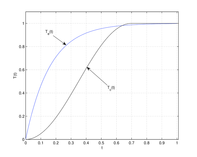
Figure 10: Typical graphs of $T_{e}(t)$ and $T_{c}(t)$. Here we have set $\alpha=6.2$, $t_{0}=0.7$.

The typical graphs of $T_{c}(t)$ and $T_{e}(t)$ are shown in Figure 10. Inserting (26) into (25) yields

$$\eta(x,y,t)=\frac{1}{(2\pi)^{2}}\int\!\!\!\int\limits_{\!\!\!\!\!\mathbb{R}^{2}}\frac{\widehat{\zeta}(k,\ell)e^{i(kx+\ell y)}}{\cosh(mh)}\frac{1}{2\pi i}\int\limits_{\mu-i\infty}^{\mu+i\infty}\frac{s^{2}\mathrm{T}(s)}{s^{2}+\omega^{2}}e^{st}ds\;dkd\ell.$$ (27)

Clearly, $\eta(x,y,t)$ depends continuously on the source $\zeta(x,y)$. Physically it means that small variations of $\zeta$ (in a reasonable space of functions such as $L^{2}$) yield small variations of $\eta$. Mathematically this problem is said to be well-posed, and this property is essential for modelling the physical processes, since it means that small modifications of the ground motion (for example, the error in measurements) do not induce huge modifications of the wave patterns.

Using the special representation (26) of seabed deformation and prescribed time-dependencies, one can compute analytically the Laplace integral in (27). To perform this integration, we first have to compute the Laplace transform of $T_{i,e,c,l}(t)$. The results are

$$\mathfrak{L}[T_{i}]=\frac{1}{s},\qquad\mathfrak{L}[T_{e}]=\frac{\alpha}{s(\alpha+s)},$$

$$\mathfrak{L}[T_{c}]=(1+e^{-st_{0}})\frac{\gamma^{2}}{2s(s^{2}+\gamma^{2})}\;\;\mbox{with}\;\;\gamma=\frac{\pi}{t_{0}},\qquad\mathfrak{L}[T_{l}]=\frac{1-e^{-st_{0}}}{t_{0}s^{2}}.$$

Inserting these formulas into the inverse Laplace integral yields

$$\frac{1}{2\pi i}\int\limits_{\mu-i\infty}^{\mu+i\infty}\frac{e^{st}s^{2}\mathrm{T_{i}}(s)}{s^{2}+\omega^{2}}ds = \cos\omega t,$$

$$\frac{1}{2\pi i}\int\limits_{\mu-i\infty}^{\mu+i\infty}\frac{e^{st}s^{2}\mathrm{T_{e}}(s)}{s^{2}+\omega^{2}}ds = -\frac{\alpha^{2}}{\alpha^{2}+\omega^{2}}\left(e^{-\alpha t}-\cos\omega t-\frac{\omega}{\alpha}\sin\omega t\right),$$

$$\frac{1}{2\pi i}\int\limits_{\mu-i\infty}^{\mu+i\infty}\frac{e^{st}s^{2}\mathrm{T_{c}}(s)}{s^{2}+\omega^{2}}ds = \frac{\gamma^{2}}{2(\gamma^{2}-\omega^{2})}$$

$$\left(\cos\omega t-\cos\gamma t+H(t-t_{0})[\cos\omega(t-t_{0})+\cos\gamma t]\right),$$

$$\frac{1}{2\pi i}\int\limits_{\mu-i\infty}^{\mu+i\infty}\frac{e^{st}s^{2}\mathrm{T_{l}}(s)}{s^{2}+\omega^{2}}ds = \frac{\sin\omega t-H(t-t_{0})\sin\omega(t-t_{0})}{\omega t_{0}}.$$

The final integral formulas for the free-surface elevations with different time dependencies are as follows:

$$\eta_{i}(x,y,t) = \frac{1}{(2\pi)^{2}}\int\!\!\!\int\limits_{\!\!\!\!\!\mathbb{R}^{2}}\frac{\widehat{\zeta}(k,\ell)e^{i(kx+\ell y)}}{\cosh(mh)}\cos\omega t\;dkd\ell,$$

$$\eta_{e}(x,y,t) = \frac{-\alpha^{2}}{(2\pi)^{2}}\int\!\!\!\int\limits_{\!\!\!\!\!\mathbb{R}^{2}}\frac{\widehat{\zeta}(k,\ell)e^{i(kx+\ell y)}}{\cosh(mh)}\left(\frac{e^{-\alpha t}-\cos\omega t-\frac{\omega}{\alpha}\sin\omega t}{\alpha^{2}+\omega^{2}}\right)\;dkd\ell,$$

$$\eta_{c}(x,y,t) = \frac{\gamma^{2}}{(2\pi)^{2}}\int\!\!\!\int\limits_{\!\!\!\!\!\mathbb{R}^{2}}\frac{\widehat{\zeta}(k,\ell)e^{i(kx+\ell y)}}{2(\gamma^{2}-\omega^{2})\cosh(mh)}$$

$$\hskip 14.22636pt\left(\cos\omega t-\cos\gamma t+H(t-t_{0})[\cos\omega(t-t_{0})+\cos\gamma t]\right)\;dkd\ell,$$

$$\eta_{l}(x,y,t) = \frac{1}{(2\pi)^{2}}\int\!\!\!\int\limits_{\!\!\!\!\!\mathbb{R}^{2}}\frac{\widehat{\zeta}(k,\ell)e^{i(kx+\ell y)}}{\cosh(mh)}\left(\frac{\sin\omega t-H(t-t_{0})\sin\omega(t-t_{0})}{\omega t_{0}}\right)\;dkd\ell.$$

3.2 Velocity field

In some applications it is important to know not only the free-surface elevation but also the velocity field in the fluid domain. One of the goals of this work is to provide an initial condition for tsunami propagation codes. For the time being, tsunami modelers take initial seabed deformations and translate them directly to the free surface in order to obtain the initial condition $\eta(x,y,0)$. Since a priori there is no information on the flow velocities, they take a zero velocity field as initial condition for the velocity: $\nabla\phi(x,y,z,0)=0$. The present computations show that it is indeed a very good approximation if the generation time is short.

In equation (24), we obtained the Fourier transform of the velocity potential $\phi(x,y,z,t)$:

$$\overline{\phi}(k,\ell,z,s)=-\frac{gs\widehat{\zeta}(k,\ell)\mathrm{T}(s)}{\cosh(mh)(s^{2}+\omega^{2})}\left(\cosh(mz)-\frac{s^{2}}{gm}\sinh(mz)\right).$$ (28)

Let us evaluate the velocity field at an arbitrary level $z=\beta h$ with $-1\leq\beta\leq 0$. In the linear approximation the value $\beta=0$ corresponds to the free surface while $\beta=-1$ corresponds to the bottom. Next we introduce some notation. The horizontal velocities are denoted by $\mathbf{u}$. The horizontal gradient $(\partial/\partial x,\partial/\partial y)$ is denoted by $\nabla_{h}$. The vertical velocity component is simply $w$. The Fourier transform parameters are denoted $\mathbf{k}=(k,\ell)$.

Taking the Fourier and Laplace transforms of

$$\mathbf{u}(x,y,t)=\left.\nabla_{h}\phi(x,y,z,t)\right|_{z=\beta h}$$

yields

$$\overline{\mathbf{u}}(k,\ell,s) = -i\overline{\phi}(k,\ell,\beta h,s)\mathbf{k}$$

$$= i\frac{gs\widehat{\zeta}(k,\ell)\mathrm{T}(s)}{\cosh(mh)(s^{2}+\omega^{2})}\left(\cosh(\beta mh)-\frac{s^{2}}{gm}\sinh(\beta mh)\right)\mathbf{k}.$$

Inverting the Fourier and Laplace transforms gives the general formula for the horizontal velocities:

$$\mathbf{u}(x,y,t) = \frac{ig}{4\pi^{2}}\int\!\!\!\int\limits_{\!\!\!\!\!\mathbb{R}^{2}}\frac{\mathbf{k}\widehat{\zeta}(k,\ell)\cosh(m\beta h)e^{i(kx+\ell y)}}{\cosh(mh)}\frac{1}{2\pi i}\int\limits_{\mu-i\infty}^{\mu+i\infty}\frac{s\mathrm{T}(s)e^{st}}{s^{2}+\omega^{2}}\;ds\;d\mathbf{k}$$

$$-\frac{i}{4\pi^{2}}\int\!\!\!\int\limits_{\!\!\!\!\!\mathbb{R}^{2}}\frac{\mathbf{k}\widehat{\zeta}(k,\ell)\sinh(m\beta h)e^{i(kx+\ell y)}}{m\cosh(mh)}\frac{1}{2\pi i}\int\limits_{\mu-i\infty}^{\mu+i\infty}\frac{s^{3}\mathrm{T}(s)e^{st}}{s^{2}+\omega^{2}}\;ds\;d\mathbf{k}.$$

After a few computations, one finds the formulas for the time dependencies $T_{i}$, $T_{e}$ and $T_{l}$. For simplicity we only give the velocities along the free surface ($\beta=0$):

$$\mathbf{u}_{i}(x,y,t) = \frac{ig}{4\pi^{2}}\int\!\!\!\int\limits_{\!\!\!\!\!\mathbb{R}^{2}}\frac{\mathbf{k}\widehat{\zeta}(k,\ell)e^{i(kx+\ell y)}}{\cosh(mh)}\frac{\sin\omega t}{\omega}\;d\mathbf{k},$$

$$\mathbf{u}_{e}(x,y,t) = \frac{ig\alpha}{4\pi^{2}}\int\!\!\!\int\limits_{\!\!\!\!\!\mathbb{R}^{2}}\frac{\mathbf{k}\widehat{\zeta}(k,\ell)e^{i(kx+\ell y)}}{(\alpha^{2}+\omega^{2})\cosh(mh)}\left(e^{-\alpha t}-\cos\omega t+\frac{\alpha}{\omega}\sin\omega t\right)\;d\mathbf{k},$$

$$\mathbf{u}_{l}(x,y,t) = \frac{ig}{4t_{0}\pi^{2}}\int\!\!\!\int\limits_{\!\!\!\!\!\mathbb{R}^{2}}\frac{\mathbf{k}\widehat{\zeta}(k,\ell)e^{i(kx+\ell y)}}{\omega^{2}\cosh(mh)}$$

$$\hskip 28.45274pt\left(1-\cos\omega t-H(t-t_{0})[1-\cos\omega(t-t_{0})]\right)\;d\mathbf{k}.$$

Next we determine the vertical component of the velocity $w(x,y,z,t)$. It is easy to obtain the Fourier–Laplace transform $\overline{w}(k,\ell,z,s)$ by differentiating (28):

$$\overline{w}(k,\ell,z,s)=\frac{\partial\overline{\phi}}{\partial z}=\frac{sg\widehat{\zeta}(k,\ell)\mathrm{T}(s)}{\cosh(mh)(s^{2}+\omega^{2})}\left(\frac{s^{2}}{g}\cosh(mz)-m\sinh(mz)\right).$$

Inverting this transform yields

$$w(x,y,z,t) = \frac{1}{4\pi^{2}}\int\!\!\!\int\limits_{\!\!\!\!\!\mathbb{R}^{2}}\frac{\cosh(mz)\widehat{\zeta}(k,\ell)}{\cosh(mh)}e^{i(kx+\ell y)}\frac{1}{2\pi i}\int\limits_{\mu-i\infty}^{\mu+i\infty}\frac{s^{3}\mathrm{T}(s)e^{st}}{s^{2}+\omega^{2}}\;ds\;d\mathbf{k}$$

$$-\frac{g}{4\pi^{2}}\int\!\!\!\int\limits_{\!\!\!\!\!\mathbb{R}^{2}}\frac{m\sinh(mz)\widehat{\zeta}(k,\ell)}{\cosh(mh)}e^{i(kx+\ell y)}\frac{1}{2\pi i}\int\limits_{\mu-i\infty}^{\mu+i\infty}\frac{s\mathrm{T}(s)e^{st}}{s^{2}+\omega^{2}}\;ds\;d\mathbf{k},$$

for $-h<z\leq 0$. One can easily obtain the expression of the vertical velocity at a given vertical level by substituting $z=\beta h$ in the expression for $w$.

The easiest way to compute the vertical velocity $w$ along the free surface is to use the boundary condition (14). Indeed, the expression for $w$ can be simply derived by differentiating the known formula for $\eta_{i,e,c,l}(x,y,t)$. Note that formally the derivative gives the distributions $\delta(t)$ and $\delta(t-t_{0})$ under the integral sign. It is a consequence of the idealized time behaviour (such as the instantaneous scenario) and it is a disadvantage of the Laplace transform method. In order to avoid these distributions we can consider the solutions only for $t>0$ and $t\neq t_{0}$. From a practical point of view there is no restriction since for any $\varepsilon>0$ we can set $t=\varepsilon$ or $t=t_{0}+\varepsilon$. For small values of $\varepsilon$ this will give a very good approximation of the solution behaviour at these “critical” instants of time. Under this assumption we give the distribution-free expressions for the vertical velocity along the free surface:

$$w_{i}(x,y,t) = -\frac{1}{4\pi^{2}}\int\!\!\!\int\limits_{\!\!\!\!\!\mathbb{R}^{2}}\frac{\widehat{\zeta}(k,\ell)e^{i(kx+\ell y)}}{\cosh(mh)}\omega\sin\omega t\;d\mathbf{k},$$

$$w_{e}(x,y,t) = \frac{\alpha^{3}}{4\pi^{2}}\int\!\!\!\int\limits_{\!\!\!\!\!\mathbb{R}^{2}}\frac{\widehat{\zeta}(k,\ell)e^{i(kx+\ell y)}}{(\alpha^{2}+\omega^{2})\cosh(mh)}\left(e^{-\alpha t}+\frac{\omega^{2}}{\alpha^{2}}\cos\omega t-\frac{\omega}{\alpha}\sin\omega t\right)\;d\mathbf{k},$$

$$w_{c}(x,y,t) = -\frac{\gamma^{2}}{4\pi^{2}}\int\!\!\!\int\limits_{\!\!\!\!\!\mathbb{R}^{2}}\frac{\widehat{\zeta}(k,\ell)e^{i(kx+\ell y)}}{2(\gamma^{2}-\omega^{2})\cosh(mh)}\bigl{(}\omega\sin\omega t-\gamma\sin\gamma t$$

$$\hskip 56.9055pt+H(t-t_{0})[\omega\sin\omega(t-t_{0})+\gamma\sin\gamma t]\bigr{)}\;d\mathbf{k},$$

$$w_{l}(x,y,t) = \frac{1}{4t_{0}\pi^{2}}\int\!\!\!\int\limits_{\!\!\!\!\!\mathbb{R}^{2}}\frac{\widehat{\zeta}(k,\ell)e^{i(kx+\ell y)}}{\cosh(mh)}\left[\cos\omega t-H(t-t_{0})\cos\omega(t-t_{0})\right]\;d\mathbf{k}.$$

3.3 Pressure on the bottom

Since tsunameters have one component that measures the pressure at the bottom (bottom pressure recorder or simply BPR [40]), it is interesting to provide as well the expression $p_{b}(x,y,t)$ for the pressure at the bottom. The pressure $p(x,y,z,t)$ can be obtained from Bernoulli’s equation, which was written explicitly for the free surface in equation (11), but is valid everywhere in the fluid:

$$\frac{\partial\phi}{\partial t}+\frac{1}{2}|\nabla\phi|^{2}+gz+\frac{p}{\rho}=0.$$ (29)

After linearization, equation (29) becomes

$$\frac{\partial\phi}{\partial t}+gz+\frac{p}{\rho}=0.$$ (30)

Along the bottom, it reduces to

$$\frac{\partial\phi}{\partial t}+g(-h+\zeta)+\frac{p_{b}}{\rho}=0,\qquad z=-h.$$ (31)

The time-derivative of the velocity potential is readily available in Fourier space. Inverting the Fourier and Laplace transforms and evaluating the resulting expression at $z=-h$ gives for the four time scenarios, respectively,

$$\frac{\partial\phi_{i}}{\partial t} = -\frac{g}{(2\pi)^{2}}\int\!\!\!\int\limits_{\!\!\!\!\!\mathbb{R}^{2}}\frac{\widehat{\zeta}(k,\ell)e^{i(kx+\ell y)}}{\cosh^{2}(mh)}\cos\omega t\;d\mathbf{k},$$

$$\frac{\partial\phi_{e}}{\partial t} = \frac{g\alpha^{2}}{(2\pi)^{2}}\int\!\!\!\int\limits_{\!\!\!\!\!\mathbb{R}^{2}}\frac{\widehat{\zeta}(k,\ell)e^{i(kx+\ell y)}}{\alpha^{2}+\omega^{2}}\left(e^{-\alpha t}-\cos\omega t-\frac{\omega}{\alpha}\sin\omega t\right)\;d\mathbf{k}+\frac{\alpha^{4}}{(2\pi)^{2}}$$

$$\int\!\!\!\int\limits_{\!\!\!\!\!\mathbb{R}^{2}}\frac{\widehat{\zeta}(k,\ell)\tanh(mh)e^{i(kx+\ell y)}}{m(\alpha^{2}+\omega^{2})}\left(e^{-\alpha t}+\Bigl{(}\frac{\omega}{\alpha}\Bigr{)}^{2}\cos\omega t+\Bigl{(}\frac{\omega}{\alpha}\Bigr{)}^{3}\sin\omega t\right)\;d\mathbf{k},$$

$$\frac{\partial\phi_{l}}{\partial t} = -\frac{g}{t_{0}(2\pi)^{2}}\int\!\!\!\int\limits_{\!\!\!\!\!\mathbb{R}^{2}}\frac{\widehat{\zeta}(k,\ell)e^{i(kx+\ell y)}}{\omega\cosh^{2}(mh)}\left[\sin\omega t-H(t-t_{0})\sin\omega(t-t_{0})\right]\;d\mathbf{k}.$$

The bottom pressure deviation from the hydrostatic pressure is then given by

$$p_{b}(x,y,t)=-\left.\rho\frac{\partial\phi}{\partial t}\right|_{z=-h}-\rho g\zeta.$$

Plots of the bottom pressure will be given in Section 4.

3.4 Asymptotic analysis of integral solutions

In this subsection, we apply the method of stationary phase in order to estimate the far-field behaviour of the solutions. There is a lot of literature on this topic (see for example [41, 42, 43, 44, 45]). This method is a classical method in asymptotic analysis. To our knowledge, the stationary phase method was first used by Kelvin [46] in the context of linear water-wave theory.

The motivation to obtain asymptotic formulas for integral solutions was mainly due to numerical difficulties to calculate the solutions for large values of $x$ and $y$. From equation (25), it is clear that the integrand is highly oscillatory. In order to be able to resolve these oscillations, several discretization points are needed per period. This becomes extremely expensive as $r=\sqrt{x^{2}+y^{2}}\to\infty$. The numerical method used in the present study is based on a Filon-type quadrature formula [20] and has been adapted to double integrals with $\exp[i(kx+\ell y)]$ oscillations. The idea of this method consists in interpolating only the amplitude of the integrand at discretization points by some kind of polynomial or spline and then performing exact integration for the oscillating part of the integrand. This method seems to be quite efficient.

Let us first obtain an asymptotic representation for integral solutions of the general form

$$\eta(x,y,t)=\frac{1}{4\pi^{2}}\int\!\!\!\int\limits_{\!\!\!\!\!\mathbb{R}^{2}}\frac{\widehat{\zeta}(k,\ell)e^{i(kx+\ell y)}}{\cosh(mh)}T(m,t)\;dkd\ell,\;\ m=\sqrt{k^{2}+\ell^{2}}.$$ (32)

Comparing with equation (27) shows that $T(m,t)$ is in fact

$$T(m,t)=\frac{1}{2\pi i}\int\limits_{\mu-i\infty}^{\mu+i\infty}\frac{s^{2}\mathrm{T}(s)}{s^{2}+\omega^{2}}e^{st}\;ds.$$

For example, we showed above that for an instantaneous seabed deformation $T(m,t)=\cos\omega t$, where $\omega^{2}=gm\tanh mh$. For the time being, we do not specify the time behaviour $\mathrm{T}(s)$.

In equation (32), we switch to polar coordinates $m$ and $\psi=\arctan(\ell/k)$:

$$\eta(x,y,t) = \frac{1}{4\pi^{2}}\int\limits_{0}^{\infty}\int\limits_{0}^{2\pi}\frac{\widehat{\zeta}(m,\psi)e^{imr\cos(\varphi-\psi)}}{\cosh(mh)}T(m,t)m\;d\psi dm$$

$$= \frac{1}{4\pi^{2}}\int\limits_{0}^{\infty}\frac{mT(m,t)}{\cosh(mh)}\;dm\int\limits_{0}^{2\pi}\widehat{\zeta}(m,\psi)e^{imr\cos(\varphi-\psi)}\;d\psi,$$

where $(r,\varphi)$ are the polar coordinates of $(x,y)$. In the last expression, the phase function is $\Phi=mr\cos(\varphi-\psi)$. Stationary phase points satisfy the condition $\partial\Phi/\partial\psi=0$, which yields two phases: $\psi_{1}=\varphi$ and $\psi_{2}=\varphi+\pi$. An approximation to equation (32) is then obtained by applying the method of stationary phase to the integral over $\psi$:

$$\eta(r,\phi,t)\simeq\frac{1}{\sqrt{8\pi^{3}r}}\int\limits_{0}^{\infty}\frac{\sqrt{m}T(m,t)}{\cosh(mh)}\left(\widehat{\zeta}(m,\varphi)e^{i(\frac{\pi}{4}-mr)}+\widehat{\zeta}(m,\varphi+\pi)e^{i(mr-\frac{\pi}{4})}\right)dm.$$

This expression cannot be simplified if we do not make any further hypotheses on the function $T(m,t)$.

Since we are looking for the far field solution behaviour, the details of wave formation are not important. Thus we will assume that the initial seabed deformation is instantaneous:

$$T(m,t)=\cos\omega t=\frac{e^{i\omega t}+e^{-i\omega t}}{2}.$$

Inserting this particular function $T(m,t)$ in equation (32) yields

$$\eta(r,\varphi,t)=\frac{1}{8\pi^{2}}\bigl{(}I_{1}+I_{2}\bigr{)},$$

where

$$I_{1} = \int\limits_{0}^{\infty}\frac{m\widehat{\zeta}(m,\psi)}{\cosh(mh)}\int\limits_{0}^{2\pi}e^{i(\omega t+mr\cos(\varphi-\psi))}\;d\psi dm,$$

$$I_{2} = \int\limits_{0}^{\infty}\frac{m\widehat{\zeta}(m,\psi)}{\cosh(mh)}\int\limits_{0}^{2\pi}e^{i(-\omega t+mr\cos(\varphi-\psi))}\;d\psi dm.$$

The stationary phase function in these integrals is

$$\Phi(m,\psi)=mr\cos(\varphi-\psi)\pm\omega t,\qquad\omega^{2}(m)=gm\tanh mh.$$

The points of stationary phase are then obtained from the conditions

$$\frac{\partial\Phi}{\partial\psi}=0,\quad\frac{\partial\Phi}{\partial m}=0.$$

The first equation gives two points, $\psi_{1}=\varphi$ and $\psi_{2}=\varphi+\pi$, as before. The second condition yields

$$\frac{r}{t}\cos(\varphi-\psi_{1,2})=\mp\frac{d\omega}{dm}.$$ (33)

Since $d\omega/dm$ decreases from $\sqrt{gh}$ to 0 as $m$ goes from 0 to $\infty$ (see Figure 9), this equation has a unique solution for $m$ if $\left|r/t\right|\leq\sqrt{gh}$. This unique solution will be denoted by $m^{*}$.

For $\left|r\right|>t\sqrt{gh}$, there is no stationary phase. It means physically that the wave has not yet reached this region. So we can approximately set $I_{1}\approx 0$ and $I_{2}\approx 0$. From the positivity of the function $d\omega/dm$ one can deduce that $\psi_{1}=\varphi$ is a stationary phase point only for the integral $I_{2}$. Similarly, $\psi_{2}=\varphi+\pi$ is a stationary point only for the integral $I_{1}$.

Let us obtain an asymptotic formula for the first integral:

$$I_{1} \approx \int\limits_{0}^{\infty}\frac{m}{\cosh(mh)}\left(\sqrt{\frac{2\pi}{mr}}\widehat{\zeta}(m,\varphi+\pi)e^{i(\omega t-mr)}e^{i\frac{\pi}{4}}\right)\;dm$$

$$= \sqrt{\frac{2\pi}{r}}e^{i\frac{\pi}{4}}\int\limits_{0}^{\infty}\frac{\widehat{\zeta}(m,\varphi+\pi)}{\cosh(mh)}\sqrt{m}e^{i(\omega t-mr)}\;dm$$

$$\approx \sqrt{\frac{2\pi}{r}}e^{i\frac{\pi}{4}}\left(\sqrt{\frac{2\pi m^{*}}{\left|\omega^{\prime\prime}(m^{*})\right|t}}\frac{\widehat{\zeta}(m^{*},\varphi+\pi)}{\cosh(m^{*}h)}e^{i(\omega(m^{*})t-m^{*}r)}e^{-i\frac{\pi}{4}}\right)$$

$$= \frac{2\pi}{t}\sqrt{\frac{m^{*}}{-\omega^{\prime\prime}\omega^{\prime}}}\,\frac{\widehat{\zeta}(m^{*},\varphi+\pi)}{\cosh(m^{*}h)}e^{i(\omega(m^{*})t-m^{*}r)}.$$

In this estimate we have used equation (33) evaluated at the stationary phase point $(m^{*},\psi_{2})$:

$$r=t\left.\frac{d\omega}{dm}\right|_{m=m^{*}}.$$ (34)

Similarly one can obtain an estimate for the integral $I_{2}$:

$$I_{2}\approx\frac{2\pi}{t}\sqrt{\frac{m^{*}}{-\omega^{\prime\prime}\omega^{\prime}}}\,\frac{\widehat{\zeta}(m^{*},\varphi)}{\cosh(m^{*}h)}e^{-i(\omega(m^{*})t-m^{*}r)}.$$

Asymptotic values have been obtained for the integrals. As is easily observed from the expressions for $I_{1}$ and $I_{2}$, the wave train decays as $1/t$, or $1/r$, which is equivalent since $r$ and $t$ are connected by relation (34).

4 Numerical results

A lot of numerical computations based on the analytical formulas obtained in the previous sections have been performed. Because of the lack of information about the real dynamical characteristics of tsunami sources, we cannot really conclude which time dependence gives the best description of tsunami generation. At this stage it is still very difficult or even impossible.

Numerical experiments showed that the largest wave amplitudes with the time dependence $T_{c}(t)$ were obtained for relatively small values of the characteristic time $t_{0}$. The exponential dependence has shown higher amplitudes for relatively longer characteristic times. The instantaneous scenario $T_{i}$ gives at the free surface the initial seabed deformation with a slightly lower amplitude (the factor that we obtained was typically about $0.8\sim 0.94$). The water has a high-pass filter effect on the initial solid boundary deformation. The linear time dependence $T_{l}(t)$ showed a linear growth of wave amplitude from 0 to also $\approx 0.9\zeta_{0}$, where $\zeta_{0}=\max\limits_{(x,y)\in\mathbb{R}^{2}}\left|\zeta(x,y)\right|$.

In this section we provide several plots (Figure 11) of the free-surface deformation. For illustration purposes, we have chosen the instantaneous seabed deformation since it is the most widely used. The values of the parameters used in the computations are given in Table 3. We also give plots of the velocity components on the free surface a few seconds (physical) after the instantaneous deformation (Figure 12). Finally, plots of the bottom dynamic pressure are given in Figure 13.

Parameter	Value
Young modulus, $E$, GPa	9.5
Poisson ratio, $\nu$	0.27
Fault depth, $d$, km	20
Dip angle, $\delta$, ∘	13
Strike angle, $\theta$, ∘	90
Normal angle, $\phi$, ∘	0
Fault length, $L$, km	60
Fault width, $W$, km	40
Burger’s vector length, $\left|\mathbf{D}\right|$, m	15
Water depth, $h$, km	4
Acceleration due to gravity, $g$, $m/s^{2}$	9.8
Wave number, $k$, $1/m$	$10^{-4}$
Angular frequency, $\omega$, Hz	$10^{-2}$

Table 3: Physical parameters used in the numerical computations

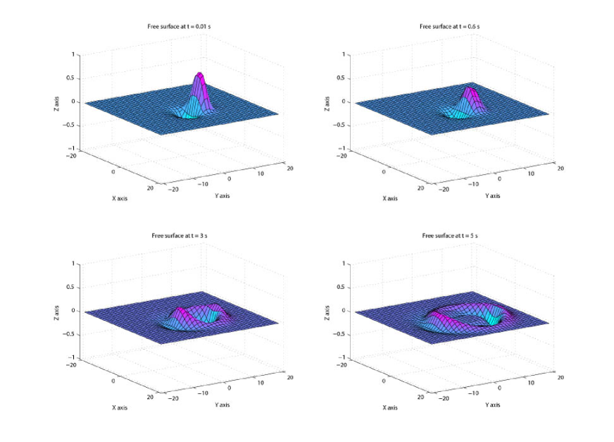
Figure 11: Free-surface elevation at $t=0.01,0.6,3,5$ in dimensionless time. In physical time it corresponds to one second, one minute, five minutes and eight minutes and a half after the initial seabed deformation.

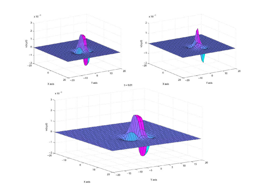
Figure 12: Components $u$, $v$ and $w$ of the velocity field computed along the free surface at $t=0.01$, that is one second after the initial seabed deformation.

From Figure 12 it is clear that the velocity field is really negligible in the beginning of wave formation. Numerical computations showed that this situation does not change if one takes other time-dependences.

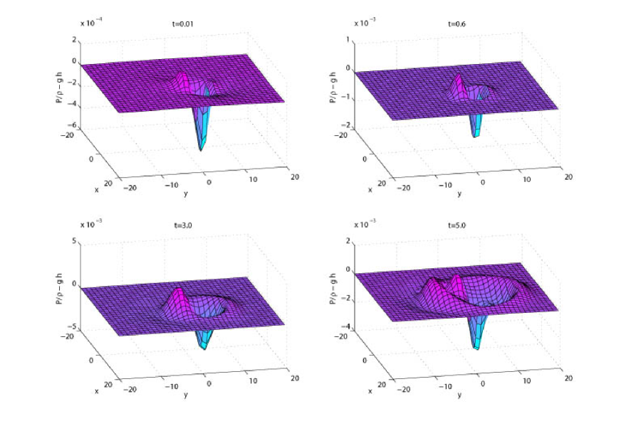
Figure 13: Bottom pressure at $t=0.01,0.6,3,5$ in dimensionless time. In physical time it corresponds to one second, one minute, five minutes and eight minutes and a half after the initial seabed deformation.

The main focus of the present paper is the generation of waves by a moving bottom. The asymptotic behaviour of various sets of initial data propagating in a fluid of uniform depth has been studied in detail by Hammack and Segur [47, 48]. In particular, they showed that the behaviours for an initial elevation wave and for an initial depression wave are different.

References

[1]
Todorovska MI, Trifunac MD (2001)
Generation of tsunamis by a slowly spreading uplift of the sea-floor.
Soil Dynamics and Earthquake Engineering
21:151–167
[2]
Neetu S, Suresh I, Shankar R, Shankar D, Shenoi SSC, Shetye SR, Sundar D, Nagarajan B (2005)
Comment on “The Great Sumatra-Andaman Earthquake of 26 December 2004”.
Science
310:1431a-1431b
[3]
Lay T, Kanamori H, Ammon CJ, Nettles M, Ward SN, Aster RC,
Beck SL, Bilek SL, Brudzinski MR, Butler R, DeShon HR, Ekstrom G,
Satake K, Sipkin S (2005)
The great Sumatra-Andaman earthquake of 26 December 2004.
Science 308:1127–1133
[4]
Korteweg DJ, de Vries G (1895)
On the change of form of long waves advancing in a rectangular canal, and on a new type of
long stationary waves.
Phil. Mag. 39:422–443
[5]
Boussinesq MJ (1871)
Théorie de l’intumescence liquide appelée
onde solitaire ou de translation se propageant dans un canal
rectangulaire.
C.R. Acad. Sci. Paris 72:755–759
[6]
Peregrine DH (1966)
Calculations of the development of an undual bore.
J Fluid Mech 25:321–330
[7]
Benjamin TB, Bona JL, Mahony JJ (1972)
Model equations for long waves in nonlinear dispersive systems.
Philos. Trans. Royal Soc. London Ser. A 272:47–78
[8]
Podyapolsky GS (1968)
The generation of linear gravitational waves in the ocean by seismic sources in the crust.
Izvestiya, Earth Physics, Akademia Nauk SSSR 1:4–12,
in Russian
[9]
Kajiura K (1963)
The leading wave of tsunami.
Bull. Earthquake Res. Inst., Tokyo Univ. 41:535–571
[10]
Gusyakov VK (1972)
Generation of tsunami waves and ocean Rayleigh waves by submarine earthquakes.
In: Mathematical problems of geophysics, vol 3, pages 250–272,
Novosibirsk, VZ SO AN SSSR, in Russian
[11]
Alekseev AS, Gusyakov VK (1973)
Numerical modelling of tsunami and seismo-acoustic
waves generation by submarine earthquakes. In:
Theory of diffraction and wave propagation, vol 2, pages 194–197, Moscow-Erevan, in Russian
[12]
Gusyakov VK (1976)
Estimation of tsunami energy. In:
Ill-posed problems of mathematical physics and problems of interpretation of geophysical observations,
pages 46–64, Novosibirsk, VZ SO AN SSSR, in Russian
[13]
Carrier GF (1971)
The dynamics of tsunamis. In:
Mathematical Problems in the Geophysical Sciences, Lectures in Applied Mathematics, vol 13,
pages 157–187, American Mathematical Society, in Russian
[14]
van den Driessche P, Braddock RD (1972)
On the elliptic generating region of a tsunami.
J. Mar. Res. 30:217–226
[15]
Braddock RD, van den Driessche P, Peady GW (1973)
Tsunami generation.
J Fluid Mech 59:817–828
[16]
Sabatier P (1986)
Formation of waves by ground motion. In: Encyclopedia of Fluid Mechanics,
pages 723–759, Gulf Publishing Company
[17]
Hammack JL (1973)
A note on tsunamis: their generation and propagation in an ocean of uniform depth.
J Fluid Mech 60:769–799
[18]
Todorovska MI, Hayir A, Trifunac MD (2002)
A note on tsunami amplitudes above submarine slides and slumps.
Soil Dynamics and Earthquake Engineering 22:129–141
[19]
Keller JB (1961)
Tsunamis: water waves produced by earthquakes. In: Proceedings of the Conference on Tsunami Hydrodynamics 24,
pages 154–166, Institute of Geophysics, University of Hawaii
[20]
Filon LNG (1928)
On a quadrature formula for trigonometric integrals.
Proc. Royal Soc. Edinburgh 49:38–47
[21]
Ursell F (1953)
The long-wave paradox in the theory of gravity waves.
Proc. Camb. Phil. Soc. 49:685–694
[22]
Okada Y (1985)
Surface deformation due to shear and tensile faults in a half-space.
Bull. Seism. Soc. Am. 75:1135–1154
[23]
Steketee JA (1958)
On Volterra’s dislocation in a semi-infinite elastic medium.
Can. J. Phys. 36:192–205
[24]
Ben-Menahem A, Singh SJ, Solomon F (1969)
Static deformation of a spherical earth model by internal dislocations.
Bull. Seism. Soc. Am. 59:813–853
[25]
Ben-Mehanem A, Singh SJ, Solomon F (1970)
Deformation of an homogeneous earth model finite by dislocations.
Rev. Geophys. Space Phys. 8:591–632
[26]
Smylie DE, Mansinha L (1971)
The elasticity theory of dislocations in real earth models and changes
in the rotation of the earth.
Geophys. J. Royal Astr. Soc. 23:329–354
[27]
Masterlark, T (2003)
Finite element model predictions of static
deformation from dislocation sources in a subduction zone:
Sensivities to homogeneous, isotropic, Poisson-solid, and half-space
assumptions.
J. Geophys. Res. 108(B11):2540
[28]
Volterra V (1907)
Sur l’équilibre des corps élastiques multiplement connexes.
Annales Scientifiques de l’Ecole Normale Supérieure 24(3):401–517
[29]
Love AEH (1944)
A treatise on the mathematical theory of elasticity.
Dover Publications, New York
[30]
Maruyama T (1964)
Static elastic dislocations in an infinite and semi-infinite medium.
Bull. Earthquake Res. Inst., Tokyo Univ. 42:289–368
[31]
Mindlin, RD (1936)
Force at a point in the interior of a semi-infinite medium.
Physics 7:195–202
[32]
Mindlin RD, Cheng DH (1950)
Nuclei of strain in the semi-infinite solid.
J. Appl. Phys. 21:926–930
[43]
Petrashen’ GI, Latyshev KP (1971)
Asymptotic Methods and Stochastic
Models in Problems of Wave Propagation,
American Mathematical Society
[44]
Bleistein N, Handelsman RA (1986)
Asymptotic Expansions of Integrals,
Dover Publications
[45]
Egorov YuV, Shubin MA (1994)
Elements of the Modern Theory. Equations with Constant Coefficients. In:
Partial Differential Equations, Encyclopedia of Mathematical Sciences, vol 2. Springer
[46]
Kelvin Lord (W. Thomson) (1887)
On the waves produced by a single impulse in water of any depth, or in a dispersive medium.
Phil. Mag. 23(5):252–255
[47]
Hammack JL, Segur H (1974)
The Korteweg–de Vries equation and water waves. Part 2. Comparison with experiments.
J Fluid Mech 65:289–314
[48]
Hammack JL, Segur H (1978)
The Korteweg–de Vries equation and water waves. Part 3. Oscillatory waves.
J Fluid Mech 84:337–358