Secondary Instabilities in Incompressible Axisymmetric Boundary Layers: Effect of Transverse Curvature

Abstract

The incompressible boundary layer in the axial flow past a cylinder has been shown Tutty et. al.(tutty ) to be stabler than a two-dimensional boundary layer, with the helical mode being the least stable. In this paper the secondary instability of this flow is studied. The laminar flow is shown here to be always stable at high transverse curvatures to secondary disturbances, which, together with a similar observation for the linear modes implies that the flow past a thin cylinder is likely to remain laminar. The azimuthal wavenumber of the pair of least stable secondary modes ($m_{+}$ and $m_{-}$) are related to that of the primary ($n$) by $m_{+}=2n$ and $m_{-}=-n$. The base flow is shown to be inviscidly stable at any curvature.

1 Introduction

At low to moderate freestream disturbance levels, the first step in the process of transition to turbulence in a boundary layer is that at some streamwise location, the laminar flow becomes unstable to linear disturbances. While this instability and the events that follow have been investigated in great detail for two-dimensional boundary layers during the past century, much less work has been done on its axisymmetric counterpart, the incompressible boundary layer in the flow past a cylinder, notable exceptions being the early and approximate linear stability analysis of Raognv and the more recent and accurate one of Tutty et. al.tutty . In Rao’s work, the equations were not solved directly and the stability estimates had severe limitations. Tutty et. al.tutty showed that non-axisymmetric modes are less stable than axisymmetric ones. The critical Reynolds number was found to be $1060$ for the $n=1$ mode and $12439$ for $n=0$. The instability is thus of a different character from that in two-dimensional boundary layers, since Squire’s (1933) theorem, stating that the first instabilities are two-dimensional, is not applicable in this case. The expected next stage of the process of transition to turbulence, namely the secondary modes of instability, have not been studied before, to our knowledge, although the turbulent flow over a long thin cylinder has been studied by Tutty tutty08 , who computed the meanflow quantities to within experimental accuracy. Practical applications, on the other hand, are numerous. For example, the axial extent of turbulent flow would determine the signature that submarines leave behind themselves, apart from the drag. The transition to turbulence over the bodies of large fish too would be partially controlled by transverse curvature.

The secondary instability of incompressible laminar flow past an axisymmetric body is thus the focus of this paper. We present results only for the flow past a cylinder, but the equations derived here and the solution method can be used for arbitrary axisymmetric bodies. We show that the overall effect of transverse curvature on incompressible boundary layers is to stabilise secondary disturbances. Remarkably no instability is found at any Reynolds number at higher curvatures, i.e., when the boundary layer thickness becomes comparable to the body radius. This implies that the boundary layer past a thin cylinder would tend to remain laminar, or to relaminarise downstream even were it to go turbulent.

We note in contrast that longitudinal curvature, and the resulting Görtler (1940) vortices on concave walls, have been well studied (see e.g. Benmalek and Saric saric94 ) and so have instabilities in three-dimensional boundary layers due to streamline curvature itoh96 .

2 Mean flow

The unperturbed laminar flow is obtained by solving the incompressible steady boundary layer equation for the axial component of velocity:

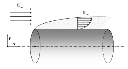
Figure 1: Schematic diagram showing the coordinate system.

$$U{{\partial U}\over{\partial x}}+V{{\partial U}\over{\partial r}}=\frac{1}{R}\Big{(}{{\partial^{2}U}\over{\partial r^{2}}}+{1\over r}{{\partial U}\over{\partial r}}\Big{)},$$ (1)

together with the continuity equation

$${{\partial U}\over{\partial x}}+{{\partial V}\over{\partial r}}+\frac{V}{r}=0,$$ (2)

and the boundary conditions

$$U(0,r)=1,\qquad U(x,1)=0,\qquad V(x,1)=0\qquad{\rm and}\qquad U(x,\infty)=1.$$ (3)

Here the $x$ coordinate is along the surface of the body and $r$ is normal to the body surface and measured from the body axis. The respective velocity components in these co-ordinates are $U$ and $V$. The length and velocity scales which have been used for non-dimensionalisation are the body radius, $r_{0}$, and the freestream velocity, $U_{\infty}$, respectively, so the Reynolds number is

$$R\equiv\frac{U_{\infty}r_{0}}{\nu}.$$ (4)

The solution is obtained by a 3-level implicit finite difference scheme on a uniform grid. At the leading edge, two levels of initial data are provided, and downstream marching is commenced. The discretised equation is second order accurate in $\Delta x$ and $\Delta r$, and is unconditionally stable in the von Neumann sense. A fairly fine grid in the $r$ direction is necessary to capture the velocity and its derivatives accurately. With a grid size of $10^{-3}$ in the $x$ and $r$ directions the results are accurate up to 7 decimal places.

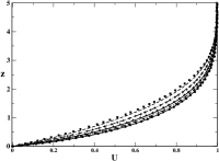
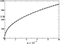
Figure 2: (a) Velocity profiles compared to those of Tutty et. al.tutty at $R=10^{4}$. The ordinate gives $z=\sqrt{R/x^{*}}(r-1)$. The lowest curve is at $x=10^{5}$ and the topmost curve is at $x=398$. The intermediate curves are spaced at intervals of $x^{1/2}$. (b) Dimensionless boundary layer thickness $\delta\sqrt{R}$ at $R=10^{4}$. In both figures, the symbols are from tutty , while the lines are present results.

Velocity profiles at a Reynolds number of $10000$ are seen in figure 2(a) to be in good agreement with the results of Tutty et. al.tutty . The dimensionless boundary layer thickness $\delta$ ($\equiv r_{0.99}-1$, where $U_{r_{0.99}}=0.99$) is plotted in figure 2(b). When scaled by the local boundary layer thickness, there is not much of a difference visible in the profiles, as seen in figure 3(a) where the Reynolds number is $4000$. Here the coordinate $r^{*}$ is measured from the body surface. A marked difference near the wall is however evident in the second derivative of the velocity (figure 3(b)). This difference is seen below to significantly affect stability behaviour. Specifically, an increasingly negative second derivative is indicative of a fuller, and therefore more stable, profile downstream.

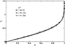
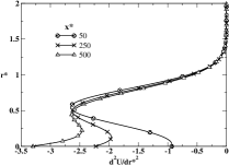
Figure 3: (a) Velocity profile at different streamwise locations, at a Reynolds number of $4000$. The coordinate $r^{*}\equiv(r-1)/\delta$. (b) Second derivative of streamwise velocity, $d^{2}U/dr^{2}$.

The boundary layer does not obey similarity, since there are two parameters in the problem, $R$ and the surface curvature $S_{0}$ defined below. Defining

$$S_{x}\equiv(4\nu x_{d}/U_{\infty}r_{0}^{2})^{1/2},$$ (5)

where the subscript $d$ denotes a dimensional quantity, we may convert the partial differential equation (1) to an ordinary differential equation in the variable $\chi=r^{2}$ ($r$ is non-dimensionalised with body radius $r_{0}$.)

$$\chi g^{\prime\prime\prime}+(1+{1\over 2S_{x}^{2}}g)g^{\prime\prime}=0.$$ (6)

Here $g^{\prime}=2U$, and the explicit dependence on $x$ is contained in $S_{x}$. It is evident that the velocity profiles would be self-similar were the quantity $x/R$ to be held constant. The momentum thickness in an axisymmetric boundary layer is of the form

$$\theta=-r_{0}+\sqrt{r_{0}^{2}+2I},\qquad{\rm where}\qquad I\equiv\int_{r_{0}}^{\infty}U(1-U)r_{d}dr_{d}.$$ (7)

The displacement thickness may be similarly defined. The surface curvature, i.e., the ratio of a typical boundary layer thickness to the body radius is defined here as

$$S_{0}\equiv\frac{\theta}{r_{0}}.$$ (8)

3 Linear stability analysis

Based on present wisdom, and our own experience in boundary layer flows, we make the assumption that non-parallel effects are small. The equations in this section are the same as those of Tutty et. al. tutty , expressed in terms of the variables introduced by Rao (1967). Flow quantities are decomposed into their mean and a fluctuating part, e.g.

$$\vec{v_{tot}} = U(r)\vec{x}+\vec{v}(x,r,\gamma,t)$$ (9)

where $\vec{v}=u\vec{x}+v\vec{r}+w\vec{\gamma}$, $\gamma$ being the azimuthal coordinate. Disturbance velocities are expressed in terms of generalized stream-functions $\psi$ and $\phi$ as

$$u={1\over r}{{{\partial\psi}\over{\partial r}}},\;v=-{1\over r}\left({{\partial\psi}\over{\partial x}}+{{\partial\phi}\over{\partial\gamma}}\right)\;{\rm and}\;w={{{\partial\phi}\over{\partial r}}}.$$ (10)

In normal mode form

$$(\psi,\phi)(x,r,\gamma)=\frac{1}{2}\Big{(}(\Psi,\Phi)(r)\exp[\rm i(\alpha x+n\gamma-\omega t)]+{\rm c.c}\Big{)}.$$ (11)

Here $\Phi(r)$ and $\Psi(r)$ are the amplitudes of the disturbance stream-functions, $\alpha$ is the wave number in the streamwise direction and $n$ is the number of waves encircling the cylinder. The value of $n$ is positive or negative for anti-clockwise or clockwise wave propagation respectively. In the temporal stability analysis carried out here, the imaginary part of the frequency $\omega$ gives the growth rate of the disturbance.

Linearising the Navier-Stokes for small disturbances and eliminating the disturbance pressure results in two fourth-order ordinary differential equations in $\Psi$ and $\Phi$, given by

$$\centering\left(U-c\right)\left(\Psi^{\prime\prime}-S\Psi^{\prime}-\alpha^{2}\Psi\right)-\Psi(U^{\prime\prime}-SU^{\prime})-\left(U-c\right)\alpha n\Phi-{n\over\alpha}\left(U^{\prime\prime}\Phi+U^{\prime}\Phi^{\prime}-SU^{\prime}\Phi\right))\@add@centering$$

$$\centering={1\over i\alpha R}\bigg{[}\Psi^{iv}-2S\Psi^{\prime\prime\prime}+3S^{2}\Psi^{\prime\prime}-3S^{3}\Psi^{\prime}-2\alpha^{2}(\Psi^{\prime\prime}-S\Psi^{\prime})+\alpha^{4}\Psi\@add@centering$$

$$\centering-n^{2}S^{2}\left(\Psi^{\prime\prime}-3S\Psi^{\prime}-\alpha^{2}\Psi\right)-n\alpha[\Phi^{\prime\prime}+S\Phi^{\prime}-(\alpha^{2}+n^{2}S^{2})\Phi]\bigg{]}\@add@centering$$ (12)

and

$$\left(U-c\right)(\Phi^{\prime\prime}+S\Phi^{\prime}-n^{2}S^{2}\Phi)+U^{\prime}\Phi^{\prime}-\left(U-c\right)n\alpha S^{2}\Psi={1\over i\alpha R}\bigg{[}\Phi^{iv}+2S\Phi^{\prime\prime\prime}$$

$$-S^{2}\Phi^{\prime\prime}(1+2n^{2})-\alpha^{2}\Phi^{\prime\prime}+S^{3}(1+2n^{2})\Phi^{\prime}-\alpha^{2}S\Phi^{\prime}-S^{4}(4n^{2}-n^{4})\Phi+\alpha^{2}n^{2}S^{2}\Phi$$

$$-n\alpha S^{2}\Psi^{\prime\prime}+3\alpha nS^{3}\Psi^{\prime}-(4\alpha nS^{4}-\alpha^{3}nS^{2}-\alpha n^{3}S^{4})\Psi\bigg{]}.$$ (13)

Here $S=\theta/r$, and the boundary conditions are

$$\Psi=\Psi^{\prime}=0,\quad\quad\Phi=\Phi^{\prime}=0\quad{\rm at}\quad r=1,$$ (14)

and

$$\Psi=\Psi^{\prime}\to 0,\quad\quad\Phi=\Phi^{\prime}\to 0\quad{\rm as}\quad r\to\infty.$$ (15)

Upon putting $S=0$ and letting $n\to\infty$ such that $nS$ tends to a finite quantity corresponding to the spanwise wavenumber, $\beta$, equations 12 and 13 reduce with some algebra to the three-dimensional Orr-Sommerfeld and Squire’s equations for boundary layers on two-dimensional surfaces (see e.g. hennibook ).

The rates of production $W_{+}(r)$ and dissipation $W_{-}(r)$ of disturbance kinetic energy are given by

$$W_{+}(r)=-{1\over 2}\Big{(}vu^{*}+v^{*}u\Big{)}{dU\over dr},$$ (16)

and,

$$W_{-}(r)={1\over Re}\Big{(}\alpha^{2}(uu^{*}+vv^{*}+ww^{*})+u^{\prime}u^{\prime*}+v^{\prime}v^{\prime*}+w^{\prime}w^{\prime*}$$

$$+{1\over r^{2}}\big{[}n^{2}uu^{*}+(1+n^{2})(vv^{*}+ww^{*})+2in(v^{*}w-vw^{*})\big{]}\Big{)}$$ (17)

where the superscript * denotes the complex conjugate. Note that the last term in 17 is derived from squares of magnitudes, and is thus real and positive.

3.1 Inviscid stability characteristics

It is instructive to first study what happens under inviscid conditions. For two-dimensional flow, the existence of a point of inflexion in the velocity profile is a necessary condition rayl for inviscid instability. The axisymmetric analog of this criterion has been derived for various situations e.g., Duck duck90 obtained the generalised criterion for axisymmetric disturbances on axisymmetric compressible boundary layers.

In brief, in the inviscid limit we may eliminate all variables except $v$ in the momentum and continuity equations for the linear perturbations, to get

$$(U-c)\left[v^{\prime\prime}+{{\left(3n^{2}+\alpha^{2}r^{2}\right)}\over{\left(\alpha^{2}r^{2}+n^{2}\right)}}{v^{\prime}\over r}-{{\left(\alpha^{2}r^{2}+n^{2}+2\right)}\over{\left(\alpha^{2}r^{2}+n^{2}\right)}}\alpha^{2}v+(1-n^{2}){v\over r^{2}}\right]-\left[U^{\prime\prime}-{{\left(\alpha^{2}r^{2}-n^{2}\right)}\over r{\left(\alpha^{2}r^{2}+n^{2}\right)}}U^{\prime}\right]v=0.$$ (18)

From a procedure similar to that for two-dimensional flows, a necessary condition for instability, that the quantity $I\equiv U^{\prime\prime}-[{{(\alpha^{2}r^{2}-n^{2})}/r/{(\alpha^{2}r^{2}+n^{2})}}]U^{\prime}$, has to change sign somewhere in the domain, is obtained. Letting $r\to\infty$, we recover the two-dimensional Rayleigh criterion.

Unlike in two-dimensional flows, the quantity $I$ depends on the streamwise and azimuthal wavenumbers, but in order to check for instability it is sufficient to evaluate the limiting cases $I_{1}$ and $I_{2}$ respectively for $\alpha/n\to 0$ and $n/\alpha\to 0$. Using equations 1 and 6, $I_{1}$ and $I_{2}$ can be written as

$$I_{1} = U^{\prime\prime}-\frac{U^{\prime}}{r}=\frac{r^{2}}{8x_{d}^{2}}g^{\prime\prime\prime},$$ (19)

$${\rm and}\quad I_{2} = U^{\prime\prime}+\frac{U^{\prime}}{r}=-\frac{1}{4Rx_{d}/r_{0}}gg^{\prime\prime}.$$ (20)

At the wall and at the freestream, $g$ and $g^{\prime\prime}$ are equal to zero, so $I_{2}$ is zero too. In between, $I_{2}$ is always negative since both $g$ and $g^{\prime\prime}$ are positive. $I_{1}$ is negative everywhere as well, i.e. $I$ never changes sign. In figure 4 these quantities are plotted for a sample case ($S_{0}=0.8$). We conclude that the incompressible axisymmetric laminar boundary layer on a circular cylinder is inviscidly stable to axisymmetric and non-axisymmetric disturbances at any curvature.

In two-dimensional boundary-layers, the inflexion point criterion has provided a general guideline for viscous flows as well, since a flow with a fuller velocity profile typically remains stable up to a much higher Reynolds number. We may therefore expect from figure 4 that an axisymmetric boundary layer will be more stable than a two-dimensional one. Also as the curvature increases (not shown) the tendency to stabilise will be higher. Note that a change of sign in $I$ may occur on converging bodies. We do not consider that case here, but mention that the axisymmetric analog of Fjortoft’s theorem,

$$(U-U_{s})\left[U^{\prime\prime}-{{(\alpha^{2}r^{2}-n^{2})}\over r{(\alpha^{2}r^{2}+n^{2})}}U^{\prime}\right]\leq 0,$$ (21)

where $U_{s}$ is the velocity at the inflection point, being a stricter criterion than the Rayleigh could then be used. The above may easily be obtained again by a procedure similar to that in two dimensions.

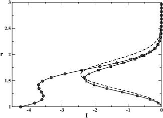
Figure 4: Sample plot of $I_{1}$ (circles) and $I_{2}$ (squares) at a Reynolds number of $5000$ and a curvature of $S_{0}=0.8$. The $U^{\prime\prime}$ of the Blasius profile is shown by the dotted line.

3.2 Numerical method and validation

Equations 12 to 15 form an eigenvalue problem, which is solved by a Chebyshev spectral collocation method. The transformation

$$y(i)=1+{\Big{(}1+y_{C}(i)\Big{)}\kappa\over 1+{2\kappa\over L}-y_{C}(i)},$$ (22)

where

$$y_{C}(i)=\cos({\pi i\over N}),\;\;\;\;\;\;i=0,1...,N.$$ (23)

are the collocation points, is used to obtain a computational domain extending from $r=1$ to $r=L+1$ and to cluster a larger number of grid points close to the wall, by a suitable choice of $\kappa$. We ensure that $L$ is at least $5$ times the boundary layer thickness, so that the far-field boundary conditions are applicable. Eigenvalues obtained using $81$ and $161$ grid points are identical up to the sixth decimal place.

	Tutty et. al. tutty				Present
$n$	$x_{c}$	$R_{c}$	$\alpha_{c}$	$c_{r}$	$x_{c}$	$R_{c}$	$\alpha_{c}$	$c_{r}$
0	47.0	12439	2.730	0.317	47.0	12463	2.730	0.318
1	543.0	1060	0.125	0.552	581.0	1013	0.115	0.552
2	91.1	6070	0.775	0.442	91.0	6093	0.775	0.421
3	43.4	10102	1.600	0.403	43.0	10110	1.580	0.410
4	26.8	13735	2.540	0.398	27.0	13742	2.520	0.401

Table 1: Critical Reynolds number and other parameters for different modes, in comparison with tutty . The streamwise location where instability first occurs is denoted as $x_{c}$. $\alpha_{c}$ and $c_{r}$ are the streamwise wavenumber and phase speed corresponding to the critical Reynolds number $R_{c}$.

We compare our critical values with those of Tutty et. al. tutty in table 1, and find them to be in reasonable agreement. The helical mode ($n=1$) is destabilised first at a Reynolds number of $1013$, and $x=581$. The axisymmetric ($n=0$) mode is unstable only above a Reynolds number of $12463$.

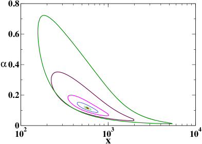
Figure 5: Neutral stability loops for the non-axisymmetric mode $n=1$ along the axial coordinate. The Reynolds number for the innermost curve is 1014 and that of the outermost curve is 5000. The Reynolds numbers for the other curves from inside to outside are 1015,1020,1060,1200 and 2000 respectively.

It is only the helical ($n=1$) mode which is unstable over a significant axial extent of the cylinder. Even this mode is never unstable for curvatures above $S_{0}=1$, as may be seen in figure 6. At curvature levels below this, as well as at low Reynolds numbers, the helical mode is expected to decide dynamics, since the ranges of instability of other modes are subsets of the range of the $n=1$ mode.

Figure 6: Critical Reynolds number as a function of curvature for the mode $n=1$.

Figure 7(a) shows the downstream variation of the critical layer location $y_{cr}$, where $U(y_{cr})=c_{r}$. It is seen that as one moves downstream, i.e., as the curvature increases for a given Reynolds number, the critical layer moves closer to the wall. Since the production layer scales as $2\pi(y_{cr}+1)r_{0}$, as the cylinder becomes thinner and thinner, the cross-sectional area over which production is possible is much smaller, explaining the stabilization at large curvature. The energy budget shows that the production layers of several unstable modes overlap, and this could give rise to interactions between them, so the nonlinear stability could be very different from that in a planar boundary layer.

Figure 7: Height of the critical layer as a function of the streamwise distance, $n=1$, $\alpha=0.125$. Dashed line: $Re=2000$; solid line $Re=10,000$.

4 Secondary instabilities

A laminar flow containing linear disturbances of a significant amplitude is unstable to secondary modes. The $\Lambda$-structures seen in kleb and Kachanov kach94 , considered to be the precursors of turbulent spots, are a signature of these modes. As a rule of thumb, nonlinearity in boundary layers becomes detectable when the amplitude of the linear (primary) disturbance is $1\%$ of the mean flow.

The approach we follow is standard, as in 88herb . The periodic basic flow is expressed as,

$$\vec{v_{basic}}=\vec{U(r)}+A_{p}\vec{v_{p}}$$ (24)

where we have introduced a subscript $p$ for the primary (linear) disturbance. $A_{p}$ is the ratio of the amplitude of disturbance velocity to the freestream velocity. $v_{p}$ is the disturbance velocity of primary modes, obtained from linear stability analysis. The secondary disturbance, in normal mode form, is

$${\vec{{v_{s}}}}=\frac{1}{2}\Big{(}\vec{v}_{+}(r)\exp[i(k_{+}x+m_{+}\theta-\omega_{+}t)]+\vec{v}_{-}(r)\exp[i(k_{-}x+m_{-}\theta-\omega_{-}t)]+{\rm c.c}\Big{)},$$ (25)

where $k_{+}$ and $+k_{-}$ are the streamwise wavenumbers of the secondary waves. The azimuthal wavenumbers of secondary waves are $m_{+}$ and $m_{-}$.

Equations for the secondary instability are obtained by substituting 24 and 25 into the Navier-Stokes equations, retaining linear terms in the secondary disturbances, and deducting the primary stability equations. The streamwise component of the velocity $u_{+}$ and $u_{-}$ are eliminated using the continuity equation. The final equations contain $v$, $w$ and $p$. On averaging over $x$, $\theta$ and $t$, only the resonant modes survive, which are related as follows:

$$k_{+}+k_{-}=\alpha,\qquad m_{+}+m_{-}=n\qquad{\rm and}\qquad(\omega_{+}+\omega_{-})_{r}=\omega.$$ (26)

The final secondary instability equations are

$$\Big{\{}(U-c)(S+D)-U^{\prime}-\frac{i}{k_{+}R}\Big{[}S\Big{(}k_{+}^{2}+(m_{+}^{2}-1)S^{2}\Big{)}+\Big{(}k_{+}^{2}+({m_{+}^{2}+1})S^{2}\Big{)}D-2SD^{2}-D^{3}\Big{]}\Big{\}}v_{+}$$

$$+\Big{\{}(U-c)im_{+}S+\frac{m_{+}S}{k_{+}R}\Big{(}k_{+}^{2}+(m_{+}^{2}-1)S^{2}+SD-D^{2}\Big{)}\Big{\}}w_{+}-ik_{+}p_{+}$$

$$+\frac{1}{2k_{-}}\Big{[}k_{+}Su_{p}+iS^{2}v_{p}-m_{-}S^{2}w_{p}+k_{-}u_{p}^{\prime}+(k_{+}u_{p}-iSv_{p}-m_{-}Sw_{p})D-iv_{p}D^{2}\Big{]}v_{-}^{*}$$

$$+\Big{[}\frac{iS}{2}\Big{(}n-\frac{k_{+}}{k_{-}}m_{-}\Big{)}u_{p}+\frac{m_{-}S^{2}}{2k_{-}}v_{p}+\frac{im_{-}^{2}S^{2}}{2k_{-}}w_{p}-\frac{m_{-}S}{2k_{-}}v_{p}D\Big{]}w_{-}^{*}=0$$ (27)

$$-\frac{2im_{+}S^{2}}{R}v_{+}+\Big{[}ik_{+}(U-c)+\frac{1}{R}\Big{(}k_{+}^{2}+(m_{+}^{2}+1)S^{2}-SD-D^{2}\Big{)}\Big{]}w_{+}+im_{+}Sp_{+}$$

$$+\Big{[}\frac{S}{2}\Big{(}\frac{\alpha}{k_{-}}-1\Big{)}w_{p}+\frac{1}{2}w_{p}^{\prime}+\frac{\alpha}{2k_{-}}w_{p}D\Big{]}v_{-}^{*}+\Big{[}-\frac{ik_{-}}{2}u_{p}+\frac{S}{2}v_{p}+\frac{iS}{2}\Big{(}m_{+}-\frac{m_{-}\alpha}{k_{-}}\Big{)}w_{p}\Big{]}w_{-}^{*}=0$$ (28)

$$\Big{[}ik_{+}(U-c)+\frac{1}{R}\Big{(}k_{+}^{2}+(m_{+}^{2}+1){S^{2}}-SD-D^{2}\Big{)}\Big{]}v_{+}+\frac{2im_{+}S^{2}}{R}w_{+}+p_{+}^{\prime}+\Big{[}-\frac{ik_{-}}{2}u_{p}$$

$$-\frac{im_{-}S}{2}w_{p}+\frac{\alpha S}{2k_{-}}v_{p}+\frac{v_{p}^{\prime}}{2}+\frac{1}{2}\Big{(}1+\frac{\alpha}{k_{-}}\Big{)}v_{p}D\Big{]}v_{-}^{*}+\Big{[}\frac{iS}{2}\Big{(}n-\frac{\alpha m_{-}}{k_{-}}\Big{)}v_{p}-\frac{Sw_{p}}{2}\Big{]}w_{-}^{*}=0$$ (29)

with three corresponding equations in $v_{-}^{*}$, $w_{-}^{*}$ and $p_{-}^{*}$. The operator $D$ stands for differentiation with respect to the radial coordinate.

The boundary conditions are

$$\vec{v_{s}}=0\quad{\rm at}\quad r=1,\qquad\vec{v_{s}}\rightarrow 0\quad{\rm as}\quad r\rightarrow\infty,\qquad{\rm and}\quad p\rightarrow 0\quad{\rm as}\quad r\rightarrow\infty.$$ (30)

For the flow under consideration, the growth/decay rates of primary modes are small, hence $d(A_{p})/dt$ can be neglected during one period of time. As mentioned above, Squires theorem does not apply and therefore the primary modes must be taken to be three-dimensional. Equations 27 to 29 reduce to the secondary instability equations of a flat plate boundary layer by letting $S=0$, $m_{+}S\to\beta$, $m_{-}S\to-\beta$ and $n_{S}=0$. The system is solved as before. Disturbance growth rates for a zero pressure gradient boundary layer agree well with those of 88herb .

4.1 Results

The main finding is that for high levels of curvature the flow is stable to secondary modes (as well as the linear modes), but secondary modes can extend the curvature range over which disturbance growth is possible. As in the case of a two-dimensional boundary layer subharmonic modes are dominant here too. The axial wavenumber of the least stable secondary mode is $k_{+}=k_{-}=\alpha/2$. At other values $k_{+}$ or $k_{-}$, the growth is smaller. This is similar to the behaviour in flat plate boundary layers. The most unstable secondary modes are of opposite obliqueness, with azimuthal wavenumber $m_{+}=2n$ and $m_{-}=-n$.

is presented in figure 8a. The amplitude $A_{p}$ of the primary wave is taken to be $2\%$ of $U_{\infty}$, but the answers do not depend qualitatively on this choice. The flow is seen to be unstable to secondary modes under conditions where all primary disturbances decay. For comparison the growth rate of the least stable primary disturbance ($\alpha=0.125$ and $n=1$) is shown as a dotted line. At small primary wave numbers the growth rate is found to be small but for a wider band of streamwise locations. As the wavenumber increases the growth rate also increases and instability is restricted to a narrow streamwise region. The maximum growth occurs when $\alpha=0.30$, and $k_{+}=k_{-}=0.15$. As discussed earlier $m_{+}=2$ and $m_{-}=-1$ in this case. It is found that the secondary modes also decay at higher curvature, but the extent of curvatures for which the instability is sustained is much larger.

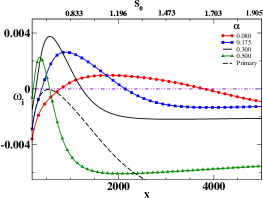
Figure 8: Growth rate of secondary disturbance waves along the cylinder axis for the non-axisymmetric mode $n=1$, $m_{-}=-1$ with $A_{p}=0.02$ at $R=1000$. The most unstable primary mode is shown by the dashed line.

In figure 9 the growth of secondary waves at higher Reynolds numbers are plotted. The flow conditions are same as in figure 8 except the Reynolds numbers. In 9a Reynolds number is 2000 while 9b is for Reynolds number 5000. The primary modes amplify substantially in these cases. The behaviour at a higher Reynolds number, as seen in figure 9, is as expected.

Incidentally a small growth is found at small curvatures (figure 9b) at this Reynolds number . However the this growth is very smaller compared to that at higher locations.

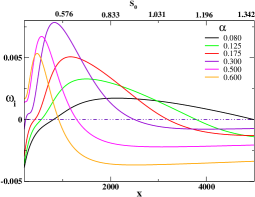
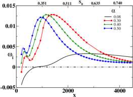
Figure 9: Growth rate of secondary disturbance along the cylinder axis for (a) $R=2000$ and (b) $R=5000$. The other parameters are the same as in figure 8.

The least stable secondary modes for other values of the azimuthal wavenumber $n$ are shown in figure 10. It is clear that in the range of Reynolds numbers of interest, these modes are not expected to dominate. The axisymmetric mode is not shown, but does not afford any surprise either.

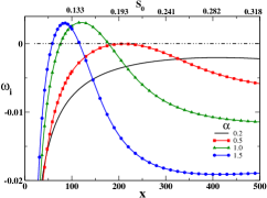
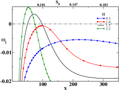
Figure 10: Growth rate of secondary disturbance modes with $A_{p}=0.02$. (a) $n=2$, $m_{+}=4$ and $m_{-}=-2$ at $R=3000$. (b) $n=3$, $m_{+}=6$ and $m_{-}=-3$ at $R=5000$.

We have computed growth rates for different modes ranging $n=1$ to $n=4$, but have shown only the results for $n=1$ and $n=2$. There is no qualitative difference in other two modes, where the relationship of $m_{+}$ to $n$ holds good.

5 Conclusions

The boundary layer in the flow past a cylinder is stable to (linear and) secondary disturbances at curvatures higher than $S_{0}\sim O(1)$, i.e. when the radius of the body is of the order of or less than the local boundary layer thickness (shown here in terms of momentum thickness). This indicates that a turbulent axisymmetric boundary layer, especially over a thin body, could have a tendency to relaminarise downstream. The flow is inviscidly stable at any curvature. Transverse curvature thus has an overall stabilising effect, acting via the mean flow and directly through the stability equations.

The production layers of the disturbance kinetic energy of these modes have a significant overlap, which gives rise to the possibility of earlier development of nonlinearities. Thus, while transverse curvature delays the first instability, it can contribute once instability sets in to a quicker and different route to turbulence.

Secondary disturbances remain unstable at larger curvatures than linear modes. However there is again a maximum curvature ($S_{0}\approx 2$ for $A_{p}=0.02$) above which all disturbances decay. The most unstable secondary modes are always those whose azimuthal wavenumbers are related to that of the primary mode by $m_{+}=2n$ and $m_{-}=-n$. For a helical primary mode (which is the most unstable) this means that one of the secondary perturbations is helical as well, but of opposite sense, while the other has the same sense but two waves straddle the body. We contrast this to a Blasius boundary layer, where the most unstable secondary mode is three-dimensional while the most unstable primary is two-dimensional. There, the spanwise wavenumber $\beta$ is of the same order as the streamwise wavenumber, and two sets of identical looking waves travel in the positive and negative spanwise directions. We do not yet have an explanation for our observation, except to say that in a coordinate moving with the primary wave, the observed most unstable secondary is the simplest combination containing one forward propagating (in the azimuthal direction) and one backward propagating wave relative to the primary. As for the axial wavenumber, the subharmonic modes are least stable, as in two-dimensional boundary layers.

Our studies indicate that experimental and numerical studies of this problem could uncover new physics about the transition to turbulence. We hazard a prediction that this process will be significantly different from two-dimensional flow.

References

- (1) Benmalek, A., Saric, W.S.: Effects of curvature variations on the nonlinear evolution of Görtler vortices. Phys Fluids 6(10), 3353–3367 (1994)
- (2) Duck, P.W.: The inviscid axisymmetric stability of the supersonic flow along a circular cylinder. J. Fluid Mech. 214, 611–637 (1990)
- (3) Herbert, T.: Secondary instability of boundary layers. Annu. Rev. Fluid Mech. 20, 487–526 (1988)
- (4) Itoh, N.: Simple cases of the streamline-curvature instability in three-dimensional boundary layers. J. Fluid Mech. 317, 129–154 (1996)
- (5) Kachanov, Y.S.: Physical mechanisms of laminar-boundary layer transition. Annu. Rev. Fluid Mech. 26, 411–482 (1994)
- (6) Klebanoff, P.S., Tidstorm, K.D., Sargent, L.M.: The three-dimensional nature of boundary layer instability. J. Fluid. Mech. 12, 1–34 (1962)
- (7) Rao, G.N.V.: Effects of convex transverse surface curvature on transition and other properties of the incompressible boundary layer. Ph.D. thesis, Dept. of Aerospace Engg., Indian Institute of Science (1967)
- (8) Rayleigh: On the stability of certain fluid motions. Proc. Math. Soc. Lond. 11, 57–70 (1880)
- (9) Schmid, P.J., Henningson, D.S.: Stability and transition in shear flows. Springer-Verlag, New York (2001)
- (10) Tutty, O.R.: Flow along a long thin cylinder. J. Fluid Mech. 602, 1–37 (2008)
- (11) Tutty, O.R., Price, W.G., Parsons, A.T.: Boundary layer flow on a long thin cylinder. Physics of Fluids 14(2), 628–637 (2002)