Taxis Equations for Amoeboid Cells

Abstract The classical macroscopic chemotaxis equations have previously been derived from an individual-based description of the tactic response of cells that use a “run-and-tumble” strategy in response to environmental cues Erban:2004:ICB ; Erban:2005:STS . Here we derive macroscopic equations for the more complex type of behavioral response characteristic of crawling cells, which detect a signal, extract directional information from a scalar concentration field, and change their motile behavior accordingly. We present several models of increasing complexity for which the derivation of population-level equations is possible, and we show how experimentally-measured statistics can be obtained from the transport equation formalism. We also show that amoeboid cells that do not adapt to constant signals can still aggregate in steady gradients, but not in response to periodic waves. This is in contrast to the case of cells that use a “run-and-tumble” strategy, where adaptation is essential.

1 Introduction

Motile organisms sense their environment and can respond to it by (i) directed movement toward or away from a signal, which is called taxis, (ii) by changing their speed of movement and/or frequency of turning, which is called kinesis, or (iii) by a combination of these. Usually these responses are both called taxes, and we adopt this convention here. Taxis involves three major components: (i) an external signal, (ii) signal transduction machinery for transducing the external signal into an internal signal, and (iii) internal components that respond to the transduced signal and lead to changes in the pattern of motility. In order to move away from noxious substances (repellents) or toward food sources (attractants) organisms must extract directional information from an extracellular scalar field, and there are two distinct strategies that are used to do this. A simple paradigm will illustrate these.

Suppose that one is close enough to a bakery to detect the odors, but cannot see the bakery. To find it, one strategy is to use sensors at the end of each arm that measure the difference in the signal at the current location and use the difference to decide on a direction. Clearly humans do not use this strategy, but instead, execute the “bakery walk”, which is to take a sniff and judge the signal intensity at the present location, take a step and another sniff, compare the signals, and from the comparison decide on the next step.

The first strategy is used by amoeboid cells (cells which move by crawling through their environment), which have receptors on the cell membrane and are large enough to detect typical differences in the signal over their body length. Small cells such as bacteria cannot effectively make a “two-point in space” measurement over their body length, and therefore they adopt the second strategy and measure the temporal variation in the signal as they move through the external field. In either case, an important consideration in understanding population-level behavior is whether or not the individual merely detects the signal and responds to it, or whether the individual alters it as well, for example by consuming it or by amplifying it so as to relay the signal. In the former case there is no feedback from the local density of individuals to the external field, but when the individual produces or degrades the signal, there is coupling between the local density of individuals and the intensity of the signal. The latter occurs, for example, when individuals move toward a signal from neighboring cells and relay the signal as well, as in the aggregation of the cellular slime mold Dictyostelium discoideum (Dd).

One of the best-characterized systems that adopts the “bakery walk” strategy is the flagellated bacterium E. coli, for which the signal transduction machinery is well characterized Bourret:2002:MIP . E. coli alternates between a more or less linear motion called a run and a highly erratic motion called tumbling, which produces little translocation but reorients the cell. Run times are typically much longer than the tumbling time, and when bacteria move in a favorable direction (i.e., either in the direction of foodstuffs or away from noxious substances), the run times are increased further. Since these bacteria are too small to detect spatial differences in the concentration of an attractant on the scale of a cell length, they choose a new direction essentially at random at the end of a tumble, although it has some bias in the direction of the preceding run Berg:1972:CEC . The effect of alternating these two modes of behavior and, in particular, of increasing the run length when moving in a favorable direction, is that a bacterium executes a three-dimensional random walk with drift in the favorable direction, when observed on a sufficiently long time scale Berg:1975:HBS ; Koshland:1980:BCM . In addition, these bacteria adapt to constant signal levels and in effect only alter the run length in response to changes in extracellular signals. Models for signal transduction and adaptation in this system has been developed Spiro:1997:MEA ; Barkai:1997:RSB , and a simplified version of the first model has been incorporated into a population-level description of behavior Erban:2004:ICB ; Erban:2005:STS . The latter analysis shows how parameters that characterize signal transduction and response in individual cells are embedded in the macroscopic sensitivity $\chi$ in the macroscopic chemotaxis equation described later. Having the bacterial example in mind, we will call the “bakery walk” strategy as a “run-and-tumble” strategy in what follows.

The directed motion of amoeboid cells (e.g. Dd or leukocytes), which is crucial in embryonic development, wound repair, the immune response to bacterial invasion, and tumor formation and metastasis, is much more complicated than bacterial motion. Cells detect extracellular chemical and mechanical signals via membrane receptors, and these trigger signal transduction cascades that produce intracellular signals. Small differences in the extracellular signal over the cell are amplified into large end-to-end intracellular differences that control the motile machinery of the cell and thereby determine the spatial localization of contact sites with the substrate and the sites of force-generation needed to produce directed motion Parent:1999:CSD ; Chung:2001:SPC . Movement of Dd and other amoeboid cells involves at least four different stages Mitchison:1996:ABC ; Sheetz:1999:CMF . (1) Cells first extend localized protrusions at the leading edge, which take the form of lamellipodia, filopodia or pseudopodia. (2) Not all protrusions are persistent, in that they must anchor to the substrate or to another cell in order for the remainder of the cell to follow Soll:1995:UCU . Protrusions are stabilized by formation of adhesive complexes, which serve as sites for molecular signaling and also transmit mechanical force to the substrate. (3) Next, in fibroblasts actomyosin filaments contract at the front of the cell and pull the cell body toward the protrusion, whereas in Dd, contraction is at the rear and the cytoplasm is squeezed forward. (4) Finally cells detach the adhesive contacts at the rear, allowing the tail of the cell to follow the main cell body. In Dd the adhesive contacts are relatively weak and the cells move rapidly ($\sim 20\mu$m/min), whereas in fibroblasts they are very strong and cells move slowly. The coordination and control of this complex process of direction sensing, amplification of spatial differences in the signal, assembly of the motile machinery, and control of the attachment to the substratum involves numerous molecules whose spatial distribution serves to distinguish the front from the rear of the cell, and whose temporal expression is tightly controlled. In addition, Dd cells adapt to the mean extracellular signal level Parent:1999:CSD .

Dd is a widely-used model system for studying signal transduction, chemotaxis, and cell motility. Dd uses cAMP as a messenger for signaling initiated by pacemaker cells to control cell movement in various stages of development (reviewed in Othmer:1998:OCS ). In the absence of cAMP stimuli Dd cells extend pseudopods in more-or-less random directions, although not strictly so since formation of a pseudopod inhibits formation of another one nearby for some time. Aggregation-competent cells respond to cAMP stimuli by suppressing existing pseudopods and rounding up (the “cringe response”), which occurs within about 20 secs and lasts about 30 secs Condeelis:1990:MAC . Under uniform elevation of the ambient cAMP this is followed by extension of pseudopods in various directions and an increase in the motility Wessels:1992:BDA ; Wessels:2000:IPR . However, one pseudopod usually dominates, even under uniform stimulation. A localized application of cAMP elicits the “cringe response” followed by a localized extension of a pseudopod near the point of application of the stimulus Swanson:1982:LSC . How the cell determines the direction in which the signal is largest, and how it organizes the motile machinery to polarize and move in that direction, are major questions from both the experimental and theoretical viewpoint. Since cAMP receptors remain uniformly distributed around the cell membrane during a tactic response, receptor localization or aggregation is not part of the response Jin:2000:LGP . Well-polarized cells are able to detect and respond to chemoattractant gradients with as little as a 2% concentration difference between the anterior and posterior of the cell Mato:1975:SIC . Directional changes of a shallow gradient induce polarized cells to turn on a time scale of 2-3 seconds Gerisch:1975:CCC , whereas large changes lead to large-scale disassembly of motile components and creation of a new “leading edge” directed toward the stimulus Gerisch:1982:CD . Polarity is labile in cells starved for short periods in that cells can rapidly change their leading edge when the stimulus is moved Swanson:1982:LSC .

There are a number of models for how cells extract directional information from the cAMP field. Fisher et  al. Fisher:1989:QAC suggest that directional information is obtained by the extension of pseudopods bearing cAMP receptors and that sensing the temporal change experienced by a receptor is equivalent to sensing the spatial gradient. However, Dd cells contain a cAMP-degrading enzyme on their surface, and it has been shown that as a result, the cAMP concentration increases in all directions normal to the cell surface Dallon:1998:CAC . Furthermore, more recent experiments show that cells in a steady gradient can polarize in the direction of the gradient without extending pseudopods Parent:1999:CSD . Thus cells must rely entirely on differences in the signal across the cell body for orientation. Moreover, the timing between different components of the response is critical, because a cell must decide how to move before it begins to relay the signal. Analysis of a model for the cAMP relay pathway shows that a cell experiences a significant difference in the front-to-back ratio of cAMP when a neighboring cell begins to signal Dallon:1998:CAC , which demonstrates that sufficient end-to-end differences for reliable orientation can be generated for typical extracellular signals. An activator-inhibitor model for an amplification step in chemotactically sensitive cells was also postulated Meinhardt:1999:OCC . Amplification of small external differences involves a Turing instability in the activator-inhibitor system, coupled to a slower inactivator that suppresses the primary activation. While this model reproduces some of the observed behavior, there is no biochemical basis for it; it is purely hypothetical and omits some of the major known processes. A model that takes into account some of the known biochemical steps has been proposed more recently Krishnan:2005:MFD .

The objective of this paper is to derive equations for the population-level behavior of amoeboid cells such as Dd or leukocytes that incorporate details about the individual-based response to signals. We present several models with the increased complexity for which the derivation of population-level equations is possible. We show how experimentally-measured statistics can be obtained from the transport equation formalism. The paper is organized as follows. We discuss the classical chemotaxis description and summarize the state of the art of the derivation of macroscopic equations and population-level statistics from individual-based models in the remainder of this section. In Section 2, we establish the general setup for models of amoeboid cells and we present individual-based models which capture the essential behavioral responses of eukaryotic cells. In Section 3 we derive the macroscopic moment equations from the microscopic model and the dependence of the mean speed on the signal strength is studied. Finally, we provide conclusions and the discussion of the presented approaches in Section 4.

1.1 Macroscopic descriptions of chemotaxis

The simplest description of cell movement in the presence of both diffusive and tactic components results by postulating that the flux of cells $\mathbf{j}$ is given by

$$\mathbf{j}=-D\nabla n+n\mathbf{u}_{c},$$ (1)

where $n$ is the density of cells, $\mathbf{u}_{c}$ is the macroscopic chemotactic velocity and $D$ is the difusion constant. The taxis is positive or negative according as $\mathbf{u}_{c}$ is parallel or anti-parallel to the direction of increase of the chemotactic substance $S$. Keller and Segel Keller:1970:ISM postulated that the chemotactic velocity is given by $\mathbf{u}_{c}=\chi(S)\nabla S$ and then (1) can be written as

$$\mathbf{j} = -D\nabla n+n\chi(S)\nabla S$$ (2)

where $\chi(S)$ is called the chemotactic sensitivity. In the absence of cell division or death the resulting conservation equation for the cell density $n(\mathbf{x},t)$ is

$$\dfrac{\partial n}{\partial t}=\nabla\cdot(D\nabla n-n\chi(S)\nabla S)$$ (3)

and this is called a classical chemotaxis equation. Unless the distribution of the chemotactic substance is fixed, (3) is coupled to an evolution equation for this substance, and perhaps other governing variables.

Other phenomenological approaches to the derivation of the chemotactic velocity have been taken. For example, by approaching taxis from a mechanical point of view, Pate and Othmer Pate:1986:DCS derived the velocity in terms of forces exerted by an amoeboid cell. Starting from Newton’s law, neglecting inertial effects, and assuming that the motive force exerted by a cell is a function of the attractant concentration, they showed how the chemotactic sensitivity is related to the rate of change of the force with attractant concentration. In this formulation the dependence of the flux on the gradient of the attractant arises from the difference in the force exerted in different directions due to different attractant concentrations. Experimental support for this comes from work of Varnum:1987:FOP , who show that as many pseudopods are produced down-gradient as up, but those up-gradient are more successful in generating cell movement. We shall use a version of the mechanical approach to taxis in a model described in the following section.

The first derivation that directly relates the chemotactic velocity to properties of individual cells is due to Patlak Patlak:1953:RWP , who used kinetic theory arguments to express ${\bf u}_{c}$ in terms of averages of the velocities and run times of individual cells. This approach was extended by Alt Alt:1980:BRW , who showed that for a class of receptor-based models the flux is approximately given by (2). These approaches are based on velocity-jump processes, which lead to transport equations of the form

$$\dfrac{\partial}{\partial t}p(\mathbf{x},\mathbf{v},t)+\mathbf{v}\cdot\nabla p(\mathbf{x},\mathbf{v},t)=-\lambda p(\mathbf{x},\mathbf{v},t)+\lambda\int_{V}T(\mathbf{v},\mathbf{v}^{\prime})p(\mathbf{x},\mathbf{v}^{\prime}\!,t)\mbox{d}\mathbf{v}^{\prime}.\;$$ (4)

where $p(\mathbf{x},\mathbf{v},t)$ is the density of cells at position $\mathbf{x}\in\Omega\subset\mathbb{R}^{n}$, moving with velocity $\mathbf{v}\in V\subset\mathbb{R}^{n}$ at time $t\geq 0$, $\lambda$ is the turning rate and kernel $T(\mathbf{v},\mathbf{v}^{\prime})$ gives the probability of a change in velocity from $\mathbf{v}^{\prime}$ to $\mathbf{v}$, given that a reorientation occurs Othmer:1988:MDB . External signals enter either through a direct effect on the turning rate $\lambda$ and the turning kernel $T$, or indirectly via internal variables that reflect the external signal and in turn influence $\lambda$ and/or $T$. The first case arises when experimental results are used to directly estimate parameters in the equation Ford:1992:SEQ , but the latter approach is more fundamental. The reduction of (4) to the macroscopic chemotaxis equations for the first case is done in Hillen:2000:DLT ; Othmer:2002:DLT and Chalub:2004:KMC .

Some statistics of the density distribution in the first case, wherein the external field modifies the turning kernel or turning rate directly, can easily be derived and used to interpret experimental data. To outline the procedure, we consider two-dimensional motion of amoeboid cells in a constant chemotactic gradient directed along the positive $x_{1}$ axis of the plane, i.e.

$$\nabla S=\,\parallel\!\!\nabla S\!\!\parallel\mathbf{e}_{1},\qquad\mbox{where we denoted}\qquad\mathbf{e}_{1}=[1,0].$$ (5)

Moreover, we assume that the gradient only influences the turn angle distribution $T$; details of the procedure are given in Othmer:1988:MDB . We assume for simplicity that the individuals move with a constant speed $s$. i.e. a velocity of an individual can be expressed as $\mathbf{v}(\phi)\equiv s[\cos(\phi),\sin(\phi)]$ where $\phi\in[0,2\pi).$ We assume that $T(\mathbf{v},\mathbf{v}^{\prime})\equiv T(\phi,\phi^{\prime})$ is the sum of a symmetric probability distribution $h(\phi)$ and a bias term $k(\phi)$ that results from the gradient of the chemotactic substance. Since the gradient is directed along the positive $x_{1}$ axis, we assume that the bias is symmetric about $\phi=0$ and takes its maximum there. Thus we write $T(\phi,\phi^{\prime})=h(\phi-\phi^{\prime})+k(\phi)$ where $h$ and $k$ are normalized as follows.

$$\int_{0}^{2\pi}h(\phi)\mbox{d}\phi=1\qquad\qquad\int_{0}^{2\pi}k(\phi)\mbox{d}\phi=0$$ (6)

Let $p(\mathbf{x},\phi,t)$ be the density of cells at position $\mathbf{x}\in\mathbb{R}^{2}$, moving with velocity $\mathbf{v}(\phi)\equiv s[\cos(\phi),\sin(\phi)]$, $\phi\in[0,2\pi)$, at time $t\geq 0$. The statistics of interest are the mean location of cells ${\mathbf{X}}(t)$, their mean squared displacement ${\cal D}^{2}(t)$, and their mean velocity ${\mathbf{V}}(t)$, which are defined as follows.

$${\mathbf{X}}(t)=\frac{1}{N_{0}}\int_{\mathbb{R}^{2}}\int_{0}^{2\pi}\mathbf{x}p(\mathbf{x},\phi,t)\,\,\mbox{d}\phi\,\mbox{d}\mathbf{x},$$

$${\cal D}^{2}(t)=\frac{1}{N_{0}}\int_{\mathbb{R}^{2}}\int_{0}^{2\pi}\parallel\!\!\mathbf{x}\!\!\parallel^{2}p(\mathbf{x},\phi,t)\,\,\mbox{d}\phi\,\mbox{d}\mathbf{x},$$

$${\mathbf{V}}(t)=\frac{1}{N_{0}}\int_{\mathbb{R}^{2}}\int_{0}^{2\pi}\mathbf{v}(\phi)p(\mathbf{x},\phi,t)\,\,\mbox{d}\phi\,\mbox{d}\mathbf{x},$$

$${\cal B}(t)=\frac{1}{N_{0}}\int_{\mathbb{R}^{2}}\int_{0}^{2\pi}(\mathbf{x}\cdot\mathbf{v}(\phi))p(\mathbf{x},\phi,t)\,\,\mbox{d}\phi\,\mbox{d}\mathbf{x},$$

where $N_{0}$ is the total number of individuals present and ${\cal{B}}(t)$ is an auxiliary variable that is needed in the analysis. Two further quantities that arise naturally are the taxis coefficient $\chi$, which is analogous to the chemotactic sensitivity defined earlier because it measures the response to a directional signal, and the persistence index $\psi_{d}$. These are defined as

$$\chi\equiv\int_{0}^{2\pi}k(\phi)\cos\phi\,\mbox{d}\phi\qquad\mbox{and }\qquad\psi_{d}=2\int_{0}^{\pi}h(\phi)\cos\phi\,\mbox{d}\phi.$$ (7)

The persistence index measures the tendency of a cell to continue in the current direction. Since we have assumed that the speed is constant, we must also assume that $\chi$ and $\psi_{d}$ satisfy the relation $\chi<1-\psi_{d}$, for otherwise the former assumption is violated (cf. (10)).

One can now show, by taking moments of (4), using (6) and symmetries of $h$ and $k$, that the moments satisfy the following evolution equations Othmer:1988:MDB .

$$\dfrac{\mbox{d}{\mathbf{X}}}{\mbox{d}t}={\mathbf{V}}\qquad \qquad\dfrac{\mbox{d}{\mathbf{V}}}{\mbox{d}t}=-\lambda_{0}{\mathbf{V}}+\lambda\chi s\mathbf{e}_{1}$$ (8)

$$\dfrac{\mbox{d}{\cal{D}}^{2}}{\mbox{d}t}=2{\cal{B}}\qquad \qquad\dfrac{\mbox{d}{\cal{B}}}{\mbox{d}t}=s^{2}-\lambda_{0}{\cal{B}}+\lambda\chi sX_{1}$$ (9)

where $\lambda_{0}\equiv\lambda(1-\psi_{d})$. The solution of (8) subject to zero initial data is

$${\mathbf{X}}(t)=sC_{I}\left(t-\dfrac{1}{\lambda_{0}}(1-e^{-\lambda_{0}t})\right)\mathbf{e}_{1},\qquad{\mathbf{V}}(t)=sC_{I}(1-e^{-\lambda_{0}t})\,\mathbf{e}_{1}$$ (10)

where $C_{I}\equiv\chi/(1-\psi_{d})$ is sometimes called the chemotropism index. Thus the mean velocity of cell movement is parallel to the direction of the chemotactic gradient and approaches ${\mathbf{V}}_{\infty}=s\,C_{I}\mathbf{e}_{1}$ as $t\rightarrow\infty$. Thus the asymptotic mean speed is the cell speed decreased by the factor $C_{I}$.

A measure of the fluctuations of the cell path around the expected value is provided by the mean square deviation, which is defined as

$$\sigma^{2}(t)=\frac{1}{N_{0}}\int_{\mathbb{R}^{2}}\int_{0}^{2\pi}\parallel\!\!\mathbf{x}-{\mathbf{X}}(t)\!\!\parallel^{2}p(\mathbf{x},\phi,t)\,\mbox{d}\phi\mbox{d}\mathbf{x}={\cal{D}}^{2}(t)-\parallel\!\!{\mathbf{X}}(t)\!\!\parallel^{2}.$$ (11)

Using (8) – (9), one also finds a differential equation for $\sigma^{2}$. Solving this equation, we find

$$\sigma^{2}\sim\displaystyle{\frac{2s^{2}}{\lambda_{0}}}\left\{(1-C_{I}^{2})t+\frac{1}{\lambda_{0}}\left(\frac{5}{2}C_{I}^{2}-1\right)\right\}\qquad\mbox{as}\qquad t\to\infty$$

and from this one can extract the diffusion coefficient as

$$D=\dfrac{2s^{2}}{\lambda_{0}}(1-C_{I}^{2}).$$

Therefore if the effect of an external gradient can be quantified experimentally and represented as the distribution $k$, the macroscopic diffusion coefficient, the persistence index, and the chemotactic sensitivity can be computed from measurements of the mean displacement, the asymptotic speed and the mean-squared displacement.

However, it is not as straightforward to derive directly the macroscopic evolution equations based on detailed models of signal transduction and response. Suppose that the internal dynamics that describe signal detection, transduction, processing and response are described by the system

$$\dfrac{\mbox{d}\mathbf{y}}{\mbox{d}t}=\mathbf{f}(\mathbf{y},S)$$ (12)

where $\mathbf{y}\in\mathbb{R}^{m}$ is the vector of internal variables and $S$ is the chemotactic substance ($S$ is extracellular cAMP for Dd aggregation). Models that describe the cAMP transduction pathway exist Martiel:1987:MBR ; Tang:1994:GPB ; Tang:1995:EOW , but for describing chemotaxis one would have to formulate a more detailed model. The form of this system can be very general but it should always have the “adaptive” property that the steady-state value (corresponding to the constant stimulus) of the appropriate internal variable (the “response regulator”) is independent of the absolute value of the stimulus, and that the steady state is globally attracting with respect to the positive cone of $\mathbb{R}^{m}$.

We showed earlier that for non-interacting walkers the internal dynamics can be incorporated in the transport equation as follows Erban:2004:ICB . Let $p(\mathbf{x},\mathbf{v},\mathbf{y},t)$ be the density of individuals in a $(2N+m)-$dimensional phase space with coordinates $[\mathbf{x},\mathbf{v},\mathbf{y}]$, where $\mathbf{x}\in\mathbb{R}^{N}$ is the position of a cell, $\mathbf{v}\in V\subset\mathbb{R}^{N}$ is its velocity and $\mathbf{y}\in Y\subset\mathbb{R}^{m}$ is its internal state, which evolves according to (12). The evolution of $p$ is governed by the transport equation

$$\frac{\partial p}{\partial t}+\nabla_{\mathbf{x}}\cdot\mathbf{v}p+\nabla_{\mathbf{y}}\cdot\mathbf{f}p=-\lambda(\mathbf{y})p+\int_{V}\lambda(\mathbf{y})T(\mathbf{v},\mathbf{v}^{\prime}\!,\mathbf{y})p(\mathbf{x},\mathbf{v}^{\prime},\mathbf{y},t)\mbox{d}\mathbf{v}^{\prime}$$ (13)

where, as before, we assume that the random velocity changes are the result of a Poisson process of intensity $\lambda(y)$. The kernel $T(\mathbf{v},\mathbf{v}^{\prime}\!,y)$ gives the probability of a change in velocity from $\mathbf{v}^{\prime}$ to $\mathbf{v},$ given that a reorientation occurs. The kernel $T$ is non-negative and satisfies the normalization condition $\int_{V}T(\mathbf{v},\mathbf{v}^{\prime},y)\mbox{d}\mathbf{v}=1.$ To connect this with the chemotaxis equation (3), we have to derive an evolution equation for the macroscopic density of individuals

$$n(\mathbf{x},t)=\int_{Y}\int_{V}p(\mathbf{x},\mathbf{v},\mathbf{y},t)\mbox{d}\mathbf{v}\mbox{d}\mathbf{y}.$$ (14)

The problem turns out to be tractable for systems that execute “run-and-tumble” motion, such as E. coli. To illustrate this, assume for simplicity that the motion is restricted to 1D, the signal is time-independent, the speed $s$ is constant, and the turning phase is neglected; the general cases are treated elsewhere Erban:2004:ICB ; Erban:2005:STS . Let $p^{+}$ (resp. $p^{-}$) be the density of individuals moving to the right (resp. left). Then (13) leads to a telegraph process described by the hyperbolic system

$$\frac{\partial p^{+}}{\partial t}+s\frac{\partial p^{+}}{\partial x}+\sum_{i=1}^{m}\frac{\partial}{\partial y_{i}}\left[f_{i}(\mathbf{y},S)p^{+}\right]=\lambda(\mathbf{y})\left[-p^{+}+p^{-}\right],$$ (15)

$$\frac{\partial p^{-}}{\partial t}-s\frac{\partial p^{-}}{\partial x}+\sum_{i=1}^{m}\frac{\partial}{\partial y_{i}}\left[f_{i}(\mathbf{y},S)p^{-}\right]=\lambda(\mathbf{y})\left[p^{+}-p^{-}\right].$$ (16)

The essential components of the internal dynamics in the bacterial context are fast excitation, followed by slower adaptation and return to the basal turning rate, and these aspects are captured in the system Othmer:1998:OCS

$$\frac{dy_{1}}{dt}=\frac{g(S(x))-(y_{1}+y_{2})}{\tau_{e}}\qquad\mbox{and}\qquad\frac{dy_{2}}{dt}=\frac{g(S(x))-y_{2}}{\tau_{a}}.$$ (17)

Here $g$ encodes the first step of signal transduction, $S$ is the chemoattractant, and $\tau_{e}$ and $\tau_{a}$ are time constants for excitation and adaptation, respectively. The component $y_{1}$ adapts perfectly to constant stimuli, i.e., the steady state response is independent of the magnitude of the stimulus $S$. To obtain a macroscopic limit equation for the total density $n(x,t)$ we incorporate the variables $y_{i}$ into the state and derive a system of four moment equations for various densities and fluxes Erban:2004:ICB . Assuming that the turning rate has the form $\lambda(y)=\lambda_{0}-by_{1}$, for $\lambda_{0}>0$, $b>0$, we show that this system reduces to the classical chemotaxis equation for large times

$$\frac{\partial n}{\partial t}=\frac{\partial}{\partial x}\left(\frac{s^{2}}{2\lambda_{0}}\frac{\partial n}{\partial x}-\left[\frac{bs^{2}\tau_{a}g^{\prime}(S(x))}{\lambda_{0}(1+2\lambda_{0}\tau_{a})(1+2\lambda_{0}\tau_{e})}\right]S^{\prime}(x)n\right)$$ (18)

where the chemotactic sensitivity is given explicitly in terms of parameters that characterize signal transduction and response. We have only used the simplified dynamics (17) to obtain the macroscopic chemotactic sensitivity, but this model captures the essential aspects for bacterial taxis Spiro:1997:MEA ; Erban:2004:ICB . An open problem is how one extracts the elementary processes of excitation and adaptation from a complex network of the type used for signal transduction in E. coli. Finally, let us note that the global existence results for (13) which is coupled with the evolution equation for the extracellular signal were recently given in Erban:2006:GER .

Equation (18) was derived for cells such as bacteria, that use the “run-and-tumble” strategy, and our objective in this paper is to attempt a similar reduction of the transport equation to a chemotaxis equation for more complex amoeboid eukaryotic cells. In the following section we introduce the general setup for studying amoeboid taxis. Then we study several “caricature” or “cartoon” models for amoeboid chemotaxis with the objective of deriving macroscopic population-level equations in each case. We start with a model which can capture interesting features of eukaryotic motility without introducing additional internal state variables, and then add internal state variables to the model.

2 Amoeboid taxis with internal variables

A fundamental assumption in the use of velocity-jump processes Othmer:1988:MDB to describe cell motion is that the jumps are instantaneous, and therefore the forces are Dirac distributions. This approximates the case in which very large forces act over very short time intervals, and even if one incorporates a resting or tumbling phase, as was done in Othmer:2002:DLT , the macroscopic description of motion is unchanged. This is appropriate for the analysis of bacterial motion (and other systems that use a “run-and-tumble” strategy), as summarized above, since the effect of the external signal is to change the rotational behavior of the flagella, and not, so far as it is understood, to affect the force generation mechanism itself. However, the situation is very different when analyzing the movement of crawling cells, for here the control of the force-generation machinery is an essential component of the response. While amoeboid cells such as Dd extend pseudopods “randomly” in the absence of signals, the direction of extension is tightly controlled in the presence of a directed external signal, and the direction in which forces are exerted on the substrate is controlled via the location of contacts with the substrate. Therefore it is appropriate to incorporate the force-generation machinery as part of the internal state, and as a first step we condense this all into a description of how the force exerted by a cell on its surroundings (and vice-versa) depends on the external signal. In reality amoeboid cells are also highly deformable, and a complete theoretical treatment of taxis at the single cell level has to take this into account. This is currently under investigation but will not be pursued here; instead we only describe the motion of the centroid of the cell. However, the following framework is sufficiently general to allow distributed internal variables within a cell.

Hereafter we use $\mathbf{y}$ as it appears in (19) to denote the chemical variables involved in signal transduction, control of actin polymerization, etc, and we denote the force per unit mass on the centroid of a cell by ${\cal F}(\mathbf{x},\mathbf{v},\mathbf{y})$. Therefore the internal state equations are given by

$$\dfrac{\mbox{d}\mathbf{y}}{\mbox{d}t}={\cal G}(\mathbf{y},S)$$ (19)

and the velocity evolves according to

$$\dfrac{\mbox{d}\mathbf{v}}{\mbox{d}t}={\cal F}(\mathbf{x},\mathbf{v},\mathbf{y}).$$ (20)

Here ${\cal G}:\mathbb{Y}\times\mathbb{S}\rightarrow\mathbb{Y}$ is in general a mapping between suitable Banach spaces and ${\cal F}:\mathbb{R}^{N}\times\mathbb{R}^{N}\times\mathbb{Y}\to\mathbb{R}^{N}$ where $N=1,2,$ or $3$ is the dimension of the physical space. This generality is needed because the variable $\mathbf{y}$ can include quantities that depend on the location in the cell or on the membrane, and which may, for example, satisfy a reaction-diffusion equation or another evolution equation.

The cell is therefore described by the position and velocity of its centroid, and the internal state $\mathbf{y}\in\mathbb{Y}.$ In some important cases described later there is a projection ${\cal P}:\mathbb{Y}\to\mathbb{Z}\subset\mathbb{Y}$ from $\mathbb{Y}$ onto a suitable finite-dimensional subspace $\mathbb{Z}$, obtained for example by considering the first few modes in a suitable basis for $\mathbb{Y}$, such that

$${\cal P}({\cal G}(\mathbf{y},S))=\mathbf{G}(\mathbf{z},S)\quad\mbox{and}\quad{\cal F}(\mathbf{x},\mathbf{v},\mathbf{y})=\mathbf{F}(\mathbf{x},\mathbf{v},\mathbf{z}),\quad\mbox{~{} where~{}}\quad\mathbf{z}\equiv{\cal P}\mathbf{y}.$$ (21)

Here $\mathbf{G}(\cdot,S):\mathbb{Z}\to\mathbb{Z}$ and $\mathbf{F}(\cdot,\cdot,\cdot):\mathbb{R}^{N}\times\mathbb{R}^{N}\times\mathbb{Z}\to\mathbb{R}^{N}$ are mappings between finite-dimensional spaces. The first equality defines the function $\mathbf{G}$, though it may of course be difficult to find when ${\cal G}$ is nonlinear. The function $\mathbf{F}$ is explicitly given by the second equality when the reduction is possible.

Given a suitable choice of the projection ${\cal P}$, we can reduce the infinite-dimensional system (19) – (20) to the following set of ordinary differential equations in finite dimensions for the description of individual cells.

$$\dfrac{\mbox{d}\mathbf{z}}{dt} = \mathbf{G}(\mathbf{z},S)$$ (22)

$$\dfrac{\mbox{d}\mathbf{v}}{\mbox{d}t} = \mathbf{F}(\mathbf{x},\mathbf{v},\mathbf{z})$$ (23)

Next, let $p(\mathbf{x},\mathbf{v},\mathbf{z},t)$ be the density of individuals which are at point $\mathbf{x}$, with velocity $\mathbf{v}$ and with the vector of reduced internal variables $\mathbf{z}$; then the transport equation (13) can be written in the form

$$\frac{\partial p}{\partial t}+\nabla_{\mathbf{x}}\cdot\mathbf{v}p+\nabla_{v}\cdot\mathbf{F}p+\nabla_{z}\cdot\mathbf{G}p=-\lambda(\mathbf{z})p+\int_{V}\lambda(\mathbf{z})T(\mathbf{v},\mathbf{v}^{\prime}\!,\mathbf{z})p(\mathbf{x},\mathbf{v}^{\prime}\!,\mathbf{z},t)\mbox{d}\mathbf{v}^{\prime}.$$ (24)

A crucial assumption for using the transport equation formalism is that the projection ${\cal P}$ exists; at present we do not know how to extend this framework to an infinite-dimensional manifold. Examples of models for which the projection ${\cal P}$ can be found will be given in the following sections, and in these cases we can use (24) as the starting point for obtaining macroscopic equations. As described earlier, the right-hand side models the instantaneous changes of direction of motion, and in the present context we use this to describe the small fluctuations due to random “errors” in the sensing of the signal and possibly to an intrinsic mechanism for random exploration of the local environment. Tranquillo and Lauffenburger Tranquillo:1987:SML developed a model of amoeboid movement that focuses specifically on the stochastic component.

A natural question is what can be done if a suitable projection ${\cal P}$ is not easily computed, or if the explicit form of $\mathbf{G}$ is impossible to obtain because of the complexity of the mapping $\cal G$. In some cases it may still be possible to describe the macroscopic-level dynamics by the evolution of a few slow variables, and by using computational equation-free methods which are currently being developed, to obtain populational level quantities without explicitly deriving the macroscopic equations (see Kevrekidis:2003:EFM ; Erban:2006:EFC ; Erban:2006:GRN and references there), using either the full model of the amoeboid cell or the best available reduction of it.

In the remainder of the paper we give examples of the reduction of (19) – (20) to the form (22) – (23) and the derivation of macroscopic equations via the transport equation (24), in order to understand how the population-level dynamics depends on the characteristics of the individual behavior. We start with a motivating example in which we further reduce the system (22) – (23) by assuming that $\dim\mathbb{Z}=1$ and that the function $\mathbf{G}$ transduces the signal directly, i.e., $\mathbf{z}\equiv S$.

2.1 A motivating example

To illustrate how the effect of acceleration of the cell can enter into the macroscopic equations, we consider the example of motion of a cell in the plane in response to a wave of a chemotactic substance. The typical response of Dd or leukocytes to a pulse-like wave of the chemoattractant can be divided into several phases depending on the position of the cell relative to the wave Geiger:2003:HPL . In Figure 1 we distinguish five different phases - denoted (A) – (E).

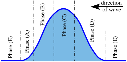
Figure 1: The notation for the different phases of the wave of chemoattractant seen by a cell at a fixed spatial position, as a function of time. The horizontal axis is the time and the vertical axis is the amplitude of the signal.

Before the wave arrives at the cell, there are no directional cues in the environment and the cell extends pseudopods in all directions – Phase (E). When the wave arrives the cell experiences an increasing temporal gradient at all points of its surface and can detect a front-to-back spatial gradient over its length (where front denotes the direction of the oncoming wave), which causes it to polarize in the direction of the oncoming wave. This is Phase (A) in Figure 1. In Phase (B) lateral pseudopod formation is suppressed and the cell moves more-or-less directly towards the aggregation center at a speed of 10-20 $\mu$m/min. In natural cAMP waves the cAMP concentration at the peak of the wave is high enough that in Phase (C) the cells stop translocating and depolarize. In Phase (D) the temporal gradient is negative, although the spatial gradient is positive in the outgoing direction, and the cell begins to form pseudopods in all directions. This is presumably due to slow adaptation to the decreasing cAMP signal, and as we shall see, if it is too fast the cells may reverse direction and follow the outgoing wave. In Phase (E), there is no extracellular signal present and there is not net movement of cells. This last phase is not described in Geiger:2003:HPL but it is of interest to include this to describe the motion in the absence of a stimulus. Formal rules used in the context of an individual-based model of Dd aggregation show that population-level aspects of chemotaxis such as stream formation can be reproduced if the foregoing phases are properly incorporated Dallon:1997:DCM . How to incorporate these characteristics into a continuum description is the question addressed here.

The following example is not meant to provide a realistic description of taxis, but rather to motivate the analysis done later. In a coarse or high-level description of movement in response to signals, information carried by the external signal detected by a cell is transduced through the intracellular signaling network, and during deterministic turns the velocity of the cell follows the external gradient with some delay. We write Newton’s law for the motion of the centroid as

$$\dfrac{\mbox{d}\mathbf{v}}{\mbox{d}t}=\dfrac{\mathbf{g}(\nabla S)-\mathbf{v}}{\tau_{v}(S)}$$ (25)

where we assume that the relaxation (or adaptation) time $\tau_{v}(S)$ is a functional of $S.$ Term $\mathbf{g}(\nabla S)$ can be interpreted in terms of the force generated from the extracellular signal. Typically $\mathbf{g}(\nabla S)$ vanishes at zero, is monotone increasing, and saturates for large $\nabla S$. The dependence of $\tau_{v}(S)$ on $S$ could arise, for instance, from different responses of the intracellular dynamics to increasing and decreasing signals; or from alterations in the adhesion sites between cell and substrate. In earlier work the turning behavior was incorporated via rules Dallon:1997:DCM , rather than via an equation of motion such as (25).

To demonstrate that this model can capture some of the salient features of Dd aggregation in response to cAMP waves from a pacemaker center, we present the results of cell-based numerical simulations that use (25) for the velocity, given a suitable choice of $\tau_{v}(S)$. We consider a two-dimensional disk (corresponding to a Petri dish) of radius $5$ mm, and we specify a periodic source of cAMP waves at the center of the domain. The period of the waves is seven minutes, their speed is $400\mu{}\mbox{m/min}$, and the maximal speed of a cell is about 20 $\mu$m per minute, all of which are chosen to approximate natural waves in a Dd aggregation field. More precisely, we choose $\mathbf{g}(\nabla S)=s_{0}\nabla S/(c_{s}+\parallel\!\!\nabla S\!\!\parallel)$ where $s_{0}=[20\mu\mbox{m/min}]$, and $c_{s}$ measures the sensitivity of the signal transduction mechanism. In the numerical examples we choose a wave with maximum $\parallel\!\!\!\nabla S\!\!\!\parallel$ equal to $1$ mm^-1 and $c_{s}=10^{-4}\mbox{mm}^{-1}$. Initially the cells are distributed uniformly and we investigate under what conditions the cells aggregate at the source of the waves of chemoattractant $S$. We consider the following two choices for the dependence of $\tau_{v}(S)$ on the external field.

(1) $\tau_{v}(S)$ is a constant independent of the signal (cf. Figure 2). In this case there is no aggregation, and in fact, cells move to the boundary of the Petri dish. This is not surprising, because cells move in the direction of the increasing gradient of the attractant, and cells first move toward the source and then turn around. Although the wave is symmetric, the cell movement creates a cellular “Doppler effect” in that there is an asymmetry in the time the cell detects the inward-directed gradient at the front of the wave versus the time it sees the receding wave. Thus in every cycle it moves away from the source longer than it moves toward it, and cells eventually accumulate at the boundary.

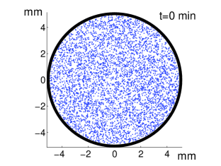
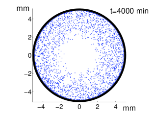
Figure 2: Simulation of $5000$ cells that move according to $(\ref{velin1})$ when the relaxation time $\tau_{v}(S)$ is constant. We plot the positions of cells at $t=0$ (left) and at $t=4000$ min (right).

(2) In this case the relaxation time is specified as a function of the time derivative of $S$ at the position of the cell, i. e., $\tau_{v}(S)\equiv\tau_{v}(S_{t})$. $\tau_{v}$ is chosen so that cells turn rapidly when the temporal derivative is positive and slowly when it is negative. In our numerical example, we simply put $\tau_{v}=0.5$ min for $S_{t}>0$, and $\tau_{v}=10$ min for $S_{t}\leq 0$. The results are shown in Figure 3; here one sees that the cells aggregate at the source of the waves.

These cases show that reorientation that is adaptive with respect to the temporal gradient of the signal suffices to produce aggregation, as was found earlier in formal cell-based rules Dallon:1997:DCM and used previously in macroscopic descriptions based on the classical chemotaxis equation Sperb:1979:MMD ; Hofer:1997:SIS .

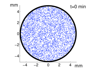
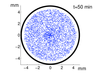
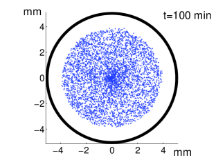
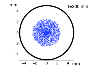
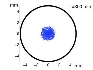
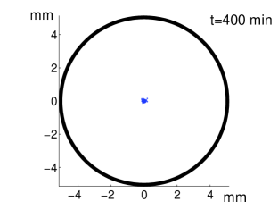
Figure 3: Simulation of cells which move according to $(\ref{velin1})$ when the relaxation time $\tau_{v}(S)\equiv\tau_{v}(S_{t})$ is chosen so that $\tau_{v}$ is small (0.5 min) when $S_{t}$ is positive and large (5 min) when $S_{t}$ is not positive. The positions of $5000$ cells at different times are plotted.

Next we address the derivation of a macroscopic description from the transport equation, using the direct effect of the signal on the turning given by (25). We denote by $p(\mathbf{x},\mathbf{v},t)$ the density of individuals which are at point $\mathbf{x}\in\mathbb{R}^{2}$ and have velocity $\mathbf{v}\in V\subset\mathbb{R}^{2}$ at time $t$. Here, $V$ is a bounded, symmetric set which is determined by the external signal and by system (25). We also assume that there is a signal-independent component to the turning for which the kernel $T$ is given by $T(\mathbf{v},\mathbf{v}^{\prime})=(2\pi v_{0})^{-1}\delta(|\mathbf{v}-\mathbf{v}^{\prime}|-v_{0})$, where $v_{0}>0$ represents the magnitude of the random component of $\mathbf{v}$. The cells add a small random component to their velocity at a rate $\lambda$. Now $p(\mathbf{x},\mathbf{v},t)$ satisfies the transport equation

$$\dfrac{\partial p}{\partial t}+\nabla_{\mathbf{x}}\cdot\mathbf{v}p+\nabla_{\mathbf{v}}\cdot\left[\left(\dfrac{\mathbf{g}(\nabla S)-\mathbf{v}}{\tau_{v}(S)}\right)p\right]=$$ (26)

$$-\lambda p(\mathbf{x},\mathbf{v},t)+\frac{\lambda}{2\pi v_{0}} \int_{V}\delta(|\mathbf{v}-\mathbf{v}^{\prime}|-v_{0})p(\mathbf{x},\mathbf{v}^{\prime}\!,t)\mbox{d}\mathbf{v}^{\prime}.$$

We define the macroscopic density $n$ and macroscopic flux $\mathbf{j}$ via

$$n=\int_{V}p(\mathbf{x},\mathbf{v},t)\mbox{d}\mathbf{v},\qquad\qquad\mathbf{j}=\int_{V}\mathbf{v}p(\mathbf{x},\mathbf{v},t)\mbox{d}\mathbf{v},$$ (27)

and by integrating (26) over $\mathbf{v},$ and multiplying (26) by $\mathbf{v}$ and integrating over $\mathbf{v},$ we obtain the following evolution equations for $n$ and $\mathbf{j}$:

$$\dfrac{\partial n}{\partial t}+\nabla_{\mathbf{x}}\cdot\mathbf{j}=0$$ (28)

$$\dfrac{\partial\mathbf{j}}{\partial t}+\nabla_{\mathbf{x}}\cdot\hat{\mathbf{j}}-\dfrac{1}{\tau_{v}(S)}\,n\,\mathbf{g}(\nabla S)=-\dfrac{\mathbf{j}}{\tau_{v}(S)}.$$ (29)

The convective flux $\hat{j}_{ik}=\int_{V}v_{i}v_{k}p(\mathbf{x},\mathbf{v},t)\mbox{d}\mathbf{v}$ that appears in (29) introduces a higher-order moment, and in earlier work on bacterial chemotaxis we could justify the closure hypothesis $j_{ik}=s^{2}n\delta_{ik}/2$, where $s$ is the speed of a bacterium (cf. Erban:2005:STS ). Since the speed is not constant during “runs” in the amoeboid case, we must use a different approach here. By constructing the evolution equation for $\hat{j}_{ik}$ and assuming that it relaxes rapidly in time, i. e., neglecting its time derivatives, and neglecting the third order velocity moments, we find that the $2\times 2$ tensor $\hat{j}$ has components

$$\hat{j}_{ik}(\mathbf{x},t)=\dfrac{\tau_{v}(S)\lambda v_{0}^{2}}{4}n\delta_{ik}+\dfrac{1}{2}\left(g_{i}j_{k}+g_{k}j_{i}\right),\qquad\mbox{for}\;i,k=1,2.$$ (30)

This leads to two possible closures, (i) by keeping only the zero-order moment (the term involving n), or (ii) by keeping both the zero-order and first-order contributions. We use the first of these here and find that the system (28) – (29) becomes

$$\dfrac{\partial n}{\partial t}+\nabla_{\mathbf{x}}\cdot\mathbf{j}=0$$ (31)

$$\dfrac{\partial\mathbf{j}}{\partial t}+\nabla\left(\dfrac{\tau_{v}(S)\lambda v_{0}^{2}}{4}n(\mathbf{x},t)\right)-\dfrac{1}{\tau_{v}(S)}\,n\,\mathbf{g}(\nabla S)=-\dfrac{\mathbf{j}}{\tau_{v}(S)}.$$ (32)

In this form we identify the chemotactic velocity and the chemotactic sensitivity as

$$\mathbf{u}_{c}=\dfrac{1}{\tau_{v}(S)}\mathbf{g}(\nabla S)\qquad\chi=\dfrac{1}{\tau_{v}(S)}\dfrac{\mathbf{g}(\nabla S)}{\nabla S}.$$

where the latter only makes sense if we assume that $\mathbf{g}(\nabla S)=g(\nabla S)\nabla S$. If in addition $g$ saturates for large arguments, the velocity saturates and the sensitivity goes to zero in the presence of large gradients, as one should expect.

One sees that at this level of closure, the relaxation rate of the flux on the right hand side of (32) is signal dependent, but if we were to suppose that $\tau_{v}(S)\equiv\tau_{0}$ is independent of $S$ then the system (31) – (32) can be written as the second order equation

$$\dfrac{\partial^{2}n}{\partial t^{2}}+\dfrac{1}{\tau_{0}}\dfrac{\partial n}{\partial t}=\dfrac{\tau_{0}\lambda v_{0}^{2}}{4}\triangle n-\nabla_{\mathbf{x}}\cdot\left(\dfrac{1}{\tau_{0}}\,n\,\mathbf{g}(\nabla S)\right),$$ (33)

which is the hyperbolic form of the classic chemotaxis equation. However, if $\tau(S)$ is signal dependent the system (31)–(32) does not reduce to (33), and this suggests that one cannot expect to obtain the classical form of the chemotaxis equation when internal states are taken into account explicitly. On the other hand, as we saw in the simulations above, one cannot avoid the “back-of-the wave paradox” without a signal-dependent $\tau_{v}$ Dallon:1997:DCM ; Dolak:2005:KMC . Let us note that we can treat similarly a modification of (25) where we allow the force to depend directly on the time derivative of the signal. This can be done by replacing $\mathbf{g}(\nabla S)$ with $\mathbf{g}(\nabla S,S_{t})$.

To illustrate the validity of the macroscopic equation (33), let us consider the cell-based numerical simulations of $N_{0}$ individuals whose velocity is governed by (25). We denote the positions of individuals as $\mathbf{x}_{i}(t)$, $i=1,\dots,N_{0}$. Then the quantities of interest are the mean position of individuals and the mean square deviation, and for the discrete-cell analysis these are defined as

$$\mathbf{X}(t)=\frac{1}{N_{0}}\sum_{i=1}^{N_{0}}\mathbf{x}_{i}(t)\qquad\mbox{and}\qquad\sigma^{2}(t)=\frac{1}{N_{0}}\sum_{i=1}^{N_{0}}\parallel\!\!\mathbf{x}_{i}(t)-{\mathbf{X}}(t)\!\!\parallel^{2}.$$ (34)

By multiplying (33) by $\mathbf{x}$ and integrating over $\mathbf{x}$, then computing the variance, much as in Section 1.1, we find that for long times the macroscopic description predicts that

$$\mathbf{X}(t)\approx\mathbf{g}(\nabla S)\,t\qquad\mbox{and}\qquad\sigma^{2}(t)\approx\tau_{0}^{2}\lambda v_{0}^{2}\,\!t.$$ (35)

To compare the theoretically-derived results (35) with the cell-based computations, we choose $\tau_{0}=1$ min, $\lambda=1\;\mbox{min}^{-1}$, $v_{0}=1\;\mu\mbox{m}/\mbox{min}$, $N_{0}=10^{4}$ cells, $\mathbf{g}=\omega{\mathbf{I}\mathbf{d}}$, where $\omega=20\;\mu\mbox{m}^{2}/$min, and $\nabla S$ is given by (5) with $\parallel\!\!\nabla S\!\!\parallel=1\;\mu\mbox{m}^{-1}$. We place all cells at $[0,0]$ and set their velocities to 0 initially, compute their subsequent motion, and plot the first component of $\mathbf{X}(t)$ and $\sigma^{2}(t)$ (as given by (34)) in Figure 4.

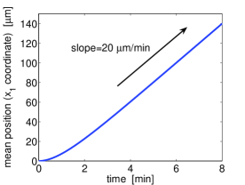
(a)   (b)

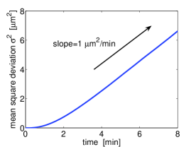
Figure 4: Time evolution of statistics $(\ref{datameanmsd})$ obtained from the cell-based simulation. (a) First component of $\mathbf{X}(t)$ as a function of time. (b) Mean square displacement $\sigma^{2}(t)$ as a function of time.

We see that after an initial transient period both quantities grow linearly with time, and the slopes are asymptotically equal to the slopes predicted theoretically using (35).

2.2 The infinite-dimensional model and its finite-dimensional reduction

As discussed earlier, analysis of E.coli chemotaxis shows that the microscopic behavior can be translated into the macroscopic parameters, and it is desirable to do the same for amoeboid chemotaxis. However, as noted earlier the internal state may now live in a Banach space, and a reduction to finite dimensions is necessary. We start with the description of excitation-adaptation dynamics on the cellular membrane to model directional sensing and reduce the resulting system. For simplicity we suppose that a cell is a disk of radius $d.$ The state of a cell will be described by the position $\mathbf{x}$ and velocity $\mathbf{v}$ of its centroid, and several internal variables on the membrane. The membrane of the cell can be described as the set

$$M=\big{\{}d\,[\cos(\theta),\sin(\theta)]\,\,|\,\,\theta\in[0,2\pi)\big{\}}.$$ (36)

The local state at each point of the membrane will be specified by the (infinite-dimensional) internal state variable $~{}~{}\mathbf{y}(\theta,t)\equiv[y_{1}(\theta,t),y_{2}(\theta,t)]^{T}$, $\theta\in[0,2\pi)$, whose evolution is governed by the “excitation-adaptation” cartoon model (17). In the formalism of equations (19) – (20) this means that the internal state $\mathbf{y}(t):[0,2\pi)\to\mathbb{R}^{2}$ can be viewed as an element of the Banach space of $2\pi$-periodic vector functions $\mathbb{Y}$ and evolves according to

$$\dfrac{\partial\mathbf{y}}{\partial t}(\theta,t)={\tilde{S}}(\theta,t){\boldsymbol{\tau}}-{\cal T}\mathbf{y}(\theta,t)$$ (37)

for $\theta\in[0,2\pi)$ and $t>0$. Here

$${\tilde{S}}(\theta,t)=S\big{(}\mathbf{x}+d~{}{\bf e}(\theta),t),\quad\quad{\bf e}(\theta)=[\cos\theta,\sin\theta]^{T},\quad\quad{\boldsymbol{\tau}}=\left[\tau_{e}^{-1},\tau_{a}^{-1}\right]^{T},$$

and

$${\cal T}\equiv\left[\begin{array}[]{cc}\tau_{e}^{-1}&\tau_{e}^{-1}\\ 0&\tau_{a}^{-1}\end{array}\right].$$

The $\mathbf{y}$-variables correspond to those in (19), and we project these to finite dimensions by considering the first Fourier mode of $y_{1}$ and the first two Fourier modes of $y_{2}$. Thus we define the average internal variables as

$$\mathbf{z}(t)=\left(z_{1}(t),z_{2}(t)\right)^{T} = \dfrac{1}{2\pi}\int_{0}^{2\pi}\mathbf{y}(\theta,t)d\theta,$$ (38)

$$\mathbf{q}(t)=\left(q_{1}(t),q_{2}(t)\right)^{T} = \dfrac{1}{d\pi}\int_{0}^{2\pi}{\bf e}(\theta)y_{2}(\theta,t)d\theta.$$ (39)

To derive equations for the reduced finite-dimensional set of internal variables $\mathbf{z}(t)$ and $\mathbf{q}(t)$, we use the approximation

$${\tilde{S}}(\theta,t)\sim S(\mathbf{x},t)+d~{}{\bf e}(\theta)\cdot\nabla S,$$ (40)

and consequently, we can write

$$\dfrac{\partial y_{2}}{\partial t}(\theta,t)=\dfrac{S(\mathbf{x},t)+d~{}{\bf e}(\theta)\cdot\nabla S-y_{2}(\theta,t)}{\tau_{a}}.$$ (41)

for $\theta\in[0,2\pi)$ , $t>0$. Multiplying (41) by 1, $\cos(\theta)$ or $\sin(\theta)$ and integrating the resulting equations with respect to $\theta,$ we obtain

$$\dfrac{\mbox{d}z_{2}}{\mbox{d}t} = \dfrac{S(\mathbf{x},t)-z_{2}}{\tau_{a}}$$ (42)

$$\dfrac{\mbox{d}\mathbf{q}}{\mbox{d}t} = \dfrac{\nabla S(\mathbf{x},t)-\mathbf{q}}{\tau_{a}},$$ (43)

Thus $z_{2}$ relaxes to the signal $S(\mathbf{x},t)$ and $\mathbf{q}$ relaxes to the directional information of $S$, both with the decay rate $\tau_{a}$. To interpret $z_{1}$, we assume fast excitation (i. e., $\tau_{e}=0).$ Then using the fact that $y_{1}={\tilde{S}}-y_{2}$ and integrating (41) with respect to $\theta$, one finds that

$$\dfrac{\mbox{d}z_{1}}{\mbox{d}t}=\dfrac{\partial S}{\partial t}(\mathbf{x},t)+\mathbf{v}\cdot\nabla S(\mathbf{x},t)-\dfrac{z_{1}}{\tau_{a}},$$ (44)

By integrating this one sees that $z_{1}$ tracks the Lagrangian derivative of $S$ taken along the cell’s trajectory, with a memory determined by $\tau_{a}$: the smaller $\tau_{a}$ the faster the cell forgets the history of this derivative. Taken together, the four variables $(z_{1},z_{2},q_{1},q_{2})$ contain information about the rate of change of the signal along the trajectory ($z_{1}$), the local value of the signal ($z_{2}$), and the gradient of the signal ($\mathbf{q}$). To this set we will add the polarization axis $\mathbf{u}=(u_{1},u_{2})$ in the next section, and the result will be the smallest set of variables that is able to capture the phenomena described earlier. Consequently, the simplest hypothesis is that cellular motility depends only on these six variables, i. e., the $\mathbf{z}$ used in (22) has six components.

2.3 The motility model

The next step is to build this model for the internal dynamics into a description of cellular movement in order to reproduce some of the experimental behaviors observed for eukaryotic chemotaxis. As we saw in Section 2.1, Dd or leukocytes respond to the waves of chemoattractant by moving toward the source of waves, and the five different stages of the wave with different behavioral responses of the cell are schematically shown in Figure 1. These and various other cell types also polarize after sufficient exposure to a directional signal Iijima:2002:TSR . In order to build directional sensing, polarization and response to waves into the model, we distinguish three distinct states of cells: (1) polarized cells which are motile (MPC), (2) polarized cells which are resting (i. e., non-motile, denoted RPC), and (3) non-polarized cells which are resting (RUC). The signal transduction machinery for all types is described by the membrane-based model (36) – (37); the difference between the types is in their motility behavior.

We describe a motile polarized cell (an MPC) by its position $\mathbf{x}$, its velocity $\mathbf{v}$ and its internal state $\mathbf{y}$, as before. However, instead of defining the force directly in terms of the signal, as was done in (25), we assume that the force is proportional to the projected internal variable $\mathbf{q}$ (defined by (39)), which tracks the gradient of the signal (cf. (43)). Thus we write the equations of motion for a cell as

$$\dfrac{\mbox{d}\mathbf{x}}{\mbox{d}t}=\mathbf{v},\qquad\dfrac{\mbox{d}\mathbf{v}}{\mbox{d}t}=\dfrac{\gamma\mathbf{q}-\mathbf{v}}{\tau_{d}}.$$ (45)

In a steady gradient of the signal $\mathbf{q}$ relaxes to $\nabla S$ on the time-scale $\tau_{a}$, and $\mathbf{v}$ relaxes to $\gamma\mathbf{q}$ on the time-scale $\tau_{d}$; thus the models predicts steady motion in a constant gradient. One expects that in general $\tau_{a}<\tau_{d}$. However, as we saw earlier, to explain the back-of-the-wave behavior Geiger:2003:HPL the response to the wave must be biased toward moving when the signal is increasing in time, as in the front of the wave. It is known that Dd cells and leukocytes stop translocating and lose their polarity in Phase (C) of a wave (cf. Figure 1), which introduces an asymmetry into the response, and to capture this we introduce a resting state. A resting cell (either an RPC or an RUC) is described by its position $\mathbf{x}$ and its internal state $\mathbf{y}\in\mathbb{Y}$, and these cells may also have a polarization axis $\mathbf{u}=(u_{1},u_{2})$. We assume that the position of a resting cell is fixed and that the internal state evolves according to (37).

Finally, we must postulate how transitions between the three states depend on the signal (cf. Figure 5). We assume that the motile cells retain their polarity upon stopping, and that the transition rate from the motile to the resting polarized state depends on $z_{1}$ as shown in Figure 5. A moving cell “computes” the directional vector $\mathbf{q}$ and the average around the perimeter of the internal variable $y_{1}$, which is $z_{1}$, according to (43) and (44).

Figure 5: The allowed transitions between cell states. The transition rates depend on the internal state $z_{1}$ as follows: $k_{21}=\lambda_{1}-b_{1}z_{1}$, $k_{12}=\lambda_{2}+b_{2}z_{1}$, $k_{13}=\lambda_{3}+b_{3}z_{1}$, $k_{32}=\lambda_{0}$.

The interpretation of Figure 5 and the justification for the postulated dependence of the transition rates between states on $z_{1}$ are as follows.

(i) If the Lagrangian derivative of the signal along a cell’s trajectory is negative, then $z_{1}$ decreases and $k_{21}$, the transition rate from the motile state to the resting polarized state, increases. The resting polarized cell adopts a polarization equal to the velocity vector before it stops, i. e., $\mathbf{u}=\mathbf{v}$ after the transition.

(ii) If a cell is resting and there is an increase in the signal, then $z_{1}$ increases and it is more likely to move. It the cell is unpolarized, than its initial velocity (polarization) is zero and the time $\tau_{d}$ reflects the time delay needed for polarization of the cell. If the cell was already polarized than its initial velocity is equal to the polarization vector, i. e.,. we set $\mathbf{v}=\mathbf{u}$, and the time delay $\tau_{d}$ reflects the relaxation time for turning, if it is necessary.

(iii) A resting polarized cell looses its polarity at a rate $\lambda_{0},$ and thus polarized cells which do not receive a stimulus for a long time lose their polarity.

Next we demonstrate that the model can successfully solve the back-of-the-wave problem Dolak:2005:KMC ; Geiger:2003:HPL , i. e., cells will aggregate at the source of the attractant waves.

2.4 Aggregation when resting states are incorporated

The internal dynamics model $\mathbf{y}$ written in terms of (19) is given by (36) – (37), and every cell is described by its position $\mathbf{x}\in\mathbb{R}^{2}$, its velocity $\mathbf{v}\in\mathbb{R}^{2}$, its polarization axis $\mathbf{u}\in\mathbb{R}^{2}$ and its internal state function $\mathbf{y}\in\mathbb{Y}$. To compute $z_{1}$ and $\mathbf{q}$, the radius of a cell is set to $d=7.5\;\mu$m, and we discretize the cell boundary (36) using $m$ meshpoints,

$$\theta_{j}=\frac{2\pi j}{m},\qquad\mbox{for}\quad j=1,2,\dots,m-1,m.$$

Then the state of each cell is described by an $(m+4)$-dimensional vector

$$(\mathbf{x},\mathbf{v},y(\theta_{1}),y(\theta_{2}),\dots,y(\theta_{m})).$$ (46)

Here, $\mathbf{v}$ denotes the velocity for an MPC and the polarization axis for an RPC. We can simply set this equal to 0 for RUCs, which are in fact described by $m+2$ variables. The internal state variables $y(\theta_{j})$ evolve according to $m$ equations of the form (37), which are uncoupled because there is no transport along the membrane. The evolution of $\mathbf{x}$ and $\mathbf{v}$ is described in Section 2.3. At each time step we use the $y(\theta_{j})$ to numerically approximate integrals (38) – (39) and thereby compute $z_{1}$, which is needed for the computation of the transition rates between different states as shown in Figure 5, and $\mathbf{q}$, which is necessary for the integration of (45). Throughout we use $m=50$, and therefore every cell is described by a $54-$dimensional state vector (46).

As was done for Figures 2 and 3, we consider a two-dimensional disk of radius $5$ mm, and we specify a periodic source of cAMP waves at the center of the domain. The period of the waves is seven minutes, their speed is $400\;\mu{}\mbox{m/min}$, and the waves are scaled so that the maximum $\parallel\!\!\nabla S\!\!\parallel$ is 1 mm^-1. Initially the cells are distributed uniformly. We use the following base transition rates and sensitivities in the transition rates $k_{ij}$ given in Figure 5:

$$\lambda_{1}=\lambda_{2}=\lambda_{3}=1\;\mbox{min}^{-1},\quad\lambda_{0}=0.2\;\mbox{min}^{-1}\quad\mbox{and}\quad b_{1}=b_{2}=b_{3}\equiv b$$ (47)

Later the parameter $b$ will be varied (cf. Figures 6 and 7). The time constants are chosen as

$$\tau_{e}=0\quad\mbox{(fast excitation)},\qquad\tau_{a}=0.5\;\mbox{min},\qquad\tau_{d}=2\;\mbox{min}.$$ (48)

The two parameters which have yet to be specified are $\gamma$ in equation (45) and $b$. The parameter $\gamma$ simply rescales the speed of cells. We know from experiments that the maximal speed of a cell is about 20 $\mu$m per minute, which can be used to fit the value of the parameter $\gamma$. We found that for $\gamma=0.08$ mm²/min, the average speed of cells on the steepest part of the wave front is between 10 $\mu$m per minute and 20 $\mu$m per minute in all simulations. Hence, we used $\gamma=0.08$ mm²/min to compute the plots shown in Figures 6 and 7.

The parameter $b$ specifies how strongly the turning rates depend on $z_{1}$ and we tested three possibilities $b=0$, $b=1\;\mbox{min}^{-1}$ and $b=2\;\mbox{min}^{-1}.$ If $b=0$ the transition rates $k_{ij}$ are independent of $z_{1}$, and the time evolution of the cell positions is shown in Figure 6. We see that in this case there is no aggregation, which is similar to what was shown earlier in Figure 2 where we considered the model without the internal dynamics and with a constant relaxation time.

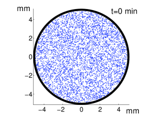
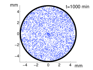
Figure 6: The cell distribution as a function of time for $b=0$. Positions of $5000$ cells at times $0$ min and $1000$ min for periodic waves of chemoattractant.

The computational results for $b=2\;\mbox{min}^{-1}$ are shown in Figure 7, where the aggregation time is comparable to the eight hours observed experimentally. The results for $b=1\;\mbox{min}^{-1}$ are similar - the only difference is that the aggregation is slower (results not shown). Using (47), we see that the transition rates (which depend on $z_{1}$) can be expressed in units of min^-1 as $k_{12}=k_{13}=1+bz_{1}$ and $k_{21}=1-bz_{1}.$ Since $bz_{1}$ is approximately in range $[-0.35,0.35]$ min^-1 for $b=1$ min^-1 and in the interval $[-0.7,0.7]$ min^-1 for $b=2$ min^-1, it implies that the turning rates are in the interval $[1-0.35,1+0.35]$ min^-1 for $b=1$ min^-1 and in the interval $[1-0.7,1+0.7]$ min^-1 for $b=2$ min^-1. As will be seen in Section 3, the moment approach used there is justified when $bz_{1}$ is small, i. e., for small bias of the turning rates. The error may increase significantly for large $b$ because the higher order moments may not be negligible.

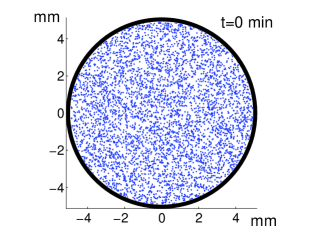
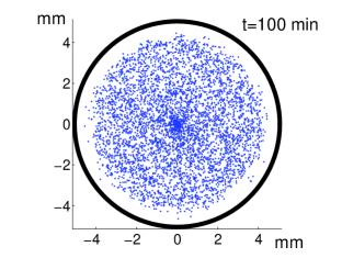
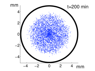
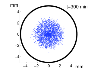
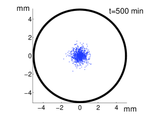
Figure 7: The cell distribution as a function of time for $b=2\;\mbox{min}^{-1}$. Positions of $5000$ cells at times $0$ min, $100$ min, $200$ min, $300$ min, $500$ min and $1000$ min for periodic waves of chemoattractant.

In these figures, as in the preceding ones related to aggregation, there is no stream formation such as is observed during aggregation of Dd. Here cells always move radially inward toward the source because the waves are imposed and are axisymmetric. In the presence of signal relay, as in Dd, it was shown earlier Lilly:2000:PFC that signal relay combined with a random initial distribution of cells plays an essential part in stream formation.

3 Transport equations

Next we show that the microscopic model for signal detection, transduction and movement can be embedded in a system of transport equations and thence into a system of moment equations for macroscopic quantities. To that end, note that every cell with the same $\mathbf{x},\mathbf{v},z_{1},\mathbf{q}$ and same polarization state will follow the same rules for movement, so it is natural to introduce density functions $p^{1},p^{2},p^{3}$ as follows:

• $p^{1}(\mathbf{x},\mathbf{v},z_{1},\mathbf{q})$ is the density of moving cells at position $\mathbf{x}$ with velocity $\mathbf{v}$ and internal moments $z_{1}$, $\mathbf{q}$;

• $p^{2}(\mathbf{x},\mathbf{u},z_{1},\mathbf{q})$ is the density of resting polarized cells at position $\mathbf{x}$ with polarization axis $\mathbf{u}$ and internal moments $z_{1}$, $\mathbf{q}$. To simplify the form of resulting transport equations, we denote the polarization axis as $\mathbf{u}\equiv\mathbf{v}$ in what follows;

• $p^{3}(\mathbf{x},z_{1},\mathbf{q})$ is the density of resting unpolarized cells at position $\mathbf{x}$ and with internal moments $z_{1}$, $\mathbf{q}$.

Hereafter we assume excitation is fast, i. e., $\tau_{e}=0,$ and we use the approximation given at (40) for the signal. The evolution of internal variables $\mathbf{q}$, $z_{1}$ is therefore given by (43) – (44). In order to simplify the following equations for $p^{1},$ $p^{2}$ and $p^{3}$, we define an operator ${\cal L}$ by

$${\cal L}r=\dfrac{\partial r}{\partial t}+\nabla_{\mathbf{q}}\cdot\left[\dfrac{1}{\tau_{a}}\left(\nabla S-\mathbf{q}\right)r\right]+\dfrac{\partial}{\partial z_{1}}\left[\left(\dfrac{\partial S}{\partial t}-\dfrac{z_{1}}{\tau_{a}}\right)r\right],$$ (49)

then the transport equations for $p^{1},$ $p^{2}$ and $p^{3}$ are

$${\cal L}p^{1} = -\nabla_{\mathbf{x}}\cdot vp^{1}-\nabla_{\mathbf{v}}\cdot\left[\dfrac{1}{\tau_{d}}\left(\gamma\mathbf{q}-\mathbf{v}\right)p^{1}\right]-\dfrac{\partial}{\partial z_{1}}\left[\left(\mathbf{v}\cdot\nabla S\right)p^{1}\right]$$ (50)

$$-(\lambda_{1}-b_{1}z_{1})p^{1}+(\lambda_{2}+b_{2}z_{1})p^{2}+\delta_{\mathbf{v}}(\lambda_{3}+b_{3}z_{1})p^{3},$$

$${\cal L}p^{2} = (\lambda_{1}-b_{1}z_{1})p^{1}-(\lambda_{2}+b_{2}z_{1})p^{2}-\lambda_{0}p^{2},$$ (51)

$${\cal L}p^{3} = \lambda_{0}\int_{V}p^{2}\mbox{d}\mathbf{v}-(\lambda_{3}+b_{3}z_{1})p^{3}.$$ (52)

where $\delta_{\mathbf{v}}$ is the Dirac function. Next we define the macroscopic densities of particles in different states as follows:

$$n^{1}(\mathbf{x},t) =\displaystyle\int_{V}\displaystyle\int_{\mathbb{R}^{3}}p^{1}(\mathbf{x},\mathbf{v},z_{1},\mathbf{q})\,\mbox{d}\mathbf{v}\mbox{d}z_{1}\mbox{d}\mathbf{q},$$ (53)

$$n^{2}(\mathbf{x},t) =\displaystyle\int_{V}\displaystyle\int_{\mathbb{R}^{3}}p^{2}(\mathbf{x},\mathbf{v},z_{1},\mathbf{q})\,\mbox{d}\mathbf{v}\mbox{d}z_{1}\mbox{d}\mathbf{q},$$ (54)

$$n^{3}(\mathbf{x},t) =\displaystyle\int_{\mathbb{R}^{3}}p^{3}(\mathbf{x},z_{1},\mathbf{q})\,\mbox{d}z_{1}\mbox{d}\mathbf{q},$$ (55)

$$n(\mathbf{x},t) =n^{1}(\mathbf{x},t)+n^{2}(\mathbf{x},t)+n^{3}(\mathbf{x},t),$$ (56)

where $n(\mathbf{x},t)$ is the total density of cells. Here and hereafter the superscript $i$ denotes a quantity associated with the $i^{th}$ species, for $i=1,2,3$. If an evolution equation in $n(\mathbf{x},t)$ alone could be found the problem would be reduced to the classical case. However we will see that this is not possible in general. First, we define some additional moments that arise in the usual manner from (50)-(52) during derivation of moment equations. More precisely, we derive the evolution equations for (53) – (56) and for the following moments

$$j^{i}_{v_{k}}(\mathbf{x},t) =\int_{V}\int_{\mathbb{R}^{3}}v_{k}p^{i}(\mathbf{x},\mathbf{v},z_{1},\mathbf{q})\mbox{d}\mathbf{v}\mbox{d}z_{1}\mbox{d}\mathbf{q},\qquad i=1,2;\;k=1,2;$$ (57)

$$n^{i}_{q_{k}}(\mathbf{x},t) =\int_{V}\int_{\mathbb{R}^{3}}q_{k}p^{i}(\mathbf{x},\mathbf{v},z_{1},\mathbf{q})\mbox{d}\mathbf{v}\mbox{d}z_{1}\mbox{d}\mathbf{q}\qquad i=1,2;\;k=1,2;$$ (58)

$$n^{i}_{z}(\mathbf{x},t) =\int_{V}\int_{\mathbb{R}^{3}}z_{1}p^{i}(\mathbf{x},\mathbf{v},z_{1},\mathbf{q})\mbox{d}\mathbf{v}\mbox{d}z_{1}\mbox{d}\mathbf{q}\qquad\qquad i=1,2;$$ (59)

$$n^{3}_{q_{k}}(\mathbf{x},t) =\int_{\mathbb{R}^{3}}q_{k}p^{3}(\mathbf{x},z_{1},\mathbf{q})\mbox{d}z_{1}\mbox{d}\mathbf{q},$$ (60)

$$n^{3}_{z}(\mathbf{x},t) =\int_{\mathbb{R}^{3}}z_{1}p^{3}(\mathbf{x},z_{1},\mathbf{q})\mbox{d}z_{1}\mbox{d}\mathbf{q}.$$ (61)

Multiplying (50)-(52) by $1$, $v_{1}$, $v_{2}$, $q_{1}$, $q_{2}$ or $z$ and integrating with respect to $\mathbf{v}$, $\mathbf{q}$ and $z_{1}$, we obtain the evolution equations for moments (53) – (61). This system of partial differential equations is not closed - it contains some higher order moments of the following form

$$m^{i}_{k_{1},k_{2},k_{3},k_{4},k_{5}}(\mathbf{x},t) = \int_{V}\int_{\mathbb{R}^{3}}v_{1}^{k_{1}}v_{2}^{k_{2}}q_{1}^{k_{3}}q_{2}^{k_{4}}z_{1}^{k_{5}}p^{i}(\mathbf{x},\mathbf{v},z_{1},\mathbf{q})\mbox{d}\mathbf{v}\mbox{d}\mathbf{q}\mbox{d}z_{1},$$

$$m^{3}_{k_{1},k_{2},k_{3}}(\mathbf{x},t) = \int_{\mathbb{R}^{3}}q_{1}^{k_{1}}q_{2}^{k_{2}}z_{1}^{k_{3}}p^{i}(\mathbf{x},\mathbf{v},z_{1},\mathbf{q})\mbox{d}\mathbf{q}\mbox{d}z_{1},$$

where $i=1,2$, $k_{\alpha}$, $\alpha=1,2,3,4,5$, are nonnegative integer, and the superscript $k_{\alpha}$ on terms in the integral denotes the $k_{\alpha}$-th power of the corresponding variable. The simplest way to close the moment equations is by setting to zero all higher-order moments which do not appear in (53) – (61). More precisely, we use the following closure assumption: $0=m^{1}_{1,1,0,0,0}=m^{1}_{2,0,0,0,0}=m^{1}_{0,2,0,0,0}=m^{1}_{1,0,1,0,0}=m^{1}_{0,1,1,0,0}=m^{1}_{1,0,0,1,0}=m^{1}_{0,1,0,1,0}=m^{1}_{1,0,0,0,1}=m^{1}_{0,1,0,0,1}=m^{1}_{0,0,1,0,1}=m^{1}_{0,0,0,1,1}=m^{1}_{0,0,0,0,2}=m^{2}_{1,0,0,0,1}=m^{2}_{0,1,0,0,1}=m^{2}_{0,0,1,0,1}=m^{2}_{0,0,0,1,1}=m^{2}_{0,0,0,0,2}=m^{3}_{1,0,1}=m^{3}_{0,1,1}=m^{3}_{0,0,2}=0.$ This closure assumption can be justified for shallow gradients of the signal Erban:2004:ICB .

Under this assumption, we multiply (50)-(52) by $1$, $v_{1}$, $v_{2}$, $q_{1}$, $q_{2}$ or $z$, we integrate with respect to $\mathbf{v}$, $\mathbf{q}$ and $z_{1}$, and we discard the higher-order moments; the result is the following closed system of 16 macroscopic equations.

$$\dfrac{\partial n^{1}}{\partial t}+\dfrac{\partial j^{1}_{v_{1}}}{\partial x_{1}}+\dfrac{\partial j^{1}_{v_{2}}}{\partial x_{2}} = -\lambda_{1}n^{1}+\lambda_{2}n^{2}+\lambda_{3}n^{3}+b_{1}n^{1}_{z}+b_{2}n^{2}_{z}+b_{3}n^{3}_{z},$$ (62)

$$\dfrac{\partial n^{2}}{\partial t}\;\phantom{+\dfrac{\partial j^{1}_{v_{1}}}{\partial x_{1}}+\dfrac{\partial j^{1}_{v_{2}}}{\partial x_{2}}} = \phantom{-}\lambda_{1}n^{1}-(\lambda_{2}+\lambda_{0})n^{2}-b_{1}n^{1}_{z}-b_{2}n^{2}_{z},$$ (63)

$$\dfrac{\partial n^{3}}{\partial t}\;\phantom{+\dfrac{\partial j^{1}_{v_{1}}}{\partial x_{1}}+\dfrac{\partial j^{1}_{v_{2}}}{\partial x_{2}}} = \phantom{-}\lambda_{0}n^{2}-\lambda_{3}n^{3}-b_{3}n^{3}_{z},$$ (64)

$$\dfrac{\partial j^{1}_{v_{k}}}{\partial t}-\dfrac{1}{\tau_{d}}\left[\gamma n^{1}_{q_{k}}-j^{1}_{v_{k}}\right] = -\lambda_{1}j^{1}_{v_{k}}+\lambda_{2}j^{2}_{v_{k}},\qquad k=1,2,$$ (65)

$$\dfrac{\partial j^{2}_{v_{k}}}{\partial t}\phantom{-\dfrac{1}{\tau_{d}}\left[\Gamma n^{1}_{q_{k}}-j^{1}_{v_{k}}\right]} = \phantom{-}\lambda_{1}j^{1}_{v_{k}}-(\lambda_{2}+\lambda_{0})j^{2}_{v_{k}},\qquad k=1,2,$$ (66)

$$\dfrac{\partial n^{1}_{q_{k}}}{\partial t}-\dfrac{1}{\tau_{a}}\dfrac{\partial S}{\partial x_{k}}n^{1}+\dfrac{1}{\tau_{a}}n^{1}_{q_{k}} = -\lambda_{1}n^{1}_{q_{k}}+\lambda_{2}n^{2}_{q_{k}}+\lambda_{3}n^{3}_{q_{k}},\qquad k=1,2,$$ (67)

$$\dfrac{\partial n^{2}_{q_{k}}}{\partial t}-\dfrac{1}{\tau_{a}}\dfrac{\partial S}{\partial x_{k}}n^{2}+\dfrac{1}{\tau_{a}}n^{2}_{q_{k}} = \phantom{-}\lambda_{1}n^{1}_{q_{k}}-(\lambda_{2}+\lambda_{0})n^{2}_{q_{k}},\qquad k=1,2,$$ (68)

$$\dfrac{\partial n^{3}_{q_{k}}}{\partial t}-\dfrac{1}{\tau_{a}}\dfrac{\partial S}{\partial x_{k}}n^{3}+\dfrac{1}{\tau_{a}}n^{3}_{q_{k}} = \phantom{-}\lambda_{0}n^{2}_{q_{k}}-\lambda_{3}n^{3}_{q_{k}},\qquad k=1,2,$$ (69)

$$\dfrac{\partial n^{1}_{z}}{\partial t}-\dfrac{\partial S}{\partial t}n^{1}+\dfrac{1}{\tau_{a}}n^{1}_{z}-\sum_{i=1}^{2}\dfrac{\partial S}{\partial x_{i}}j^{1}_{v_{i}} = -\lambda_{1}n^{1}_{z}+\lambda_{2}n^{2}_{z}+\lambda_{3}n^{3}_{z},$$ (70)

$$\dfrac{\partial n^{2}_{z}}{\partial t}-\dfrac{\partial S}{\partial t}n^{2}+\dfrac{1}{\tau_{a}}n^{2}_{z}\phantom{-\sum_{i=1}^{2}\dfrac{\partial S}{\partial x_{i}}j^{1}_{i}} = \phantom{-}\lambda_{1}n^{1}_{z}-(\lambda_{2}+\lambda_{0})n^{2}_{z},$$ (71)

$$\dfrac{\partial n^{3}_{z}}{\partial t}-\dfrac{\partial S}{\partial t}n^{3}+\dfrac{1}{\tau_{a}}n^{3}_{z}\phantom{-\sum_{i=1}^{2}\dfrac{\partial S}{\partial x_{i}}j^{1}_{i}} = \phantom{-}\lambda_{0}n^{2}_{z}-\lambda_{3}n^{3}_{z}$$ (72)

Note that the sum of equations (62) – (64) is the standard continuity equation for $n$, i. e.,

$$\dfrac{\partial n}{\partial t}+\dfrac{\partial j^{1}_{v_{1}}}{\partial x_{1}}+\dfrac{\partial j^{1}_{v_{2}}}{\partial x_{2}}=0.$$ (73)

The system (62) – (72) can be written more compactly by defining the following vectors and matrices.

$$\mathbf{n}= (n^{1},n^{2},n^{3})^{T}\qquad\quad\mathbf{n}_{z}=(n^{1}_{z},n^{2}_{z},n^{3}_{z})^{T}$$

$$\mathbf{n}_{\mathbf{q}} =(\mathbf{n}_{q_{1}},\mathbf{n}_{q_{2}})=(n_{q_{1}}^{1},n_{q_{1}}^{2}n_{q_{1}}^{3},n_{q_{2}}^{1},n_{q_{2}}^{2},n_{q_{2}}^{3})^{T}$$

$$\mathbf{j}=(\mathbf{j}_{v_{1}},\mathbf{j}_{v_{2}})^{T}=(j_{v_{1}}^{1},j_{v_{1}}^{2},j_{v_{2}}^{1},j_{v_{2}}^{2})^{T}\qquad\qquad\nabla=\left(\frac{\partial}{\partial x_{1}},\frac{\partial}{\partial x_{2}}\right)^{T}$$

$$\boldsymbol{\Lambda}=\left[\begin{array}[]{ccc}-\lambda_{1}&\lambda_{2}&\lambda_{3}\\ \lambda_{1}&-(\lambda_{2}+\lambda_{0})&0\\ 0&\lambda_{0}&-\lambda_{3}\end{array}\right]\qquad\qquad\boldsymbol{\Lambda_{1}}=\left[\begin{array}[]{cc}-\lambda_{1}&\lambda_{2}\\ \lambda_{1}&-(\lambda_{2}+\lambda_{0})\end{array}\right]$$ (74)

$${\bf B}=\left[\begin{array}[]{ccc}b_{1}&b_{2}&b_{3}\\ -b_{1}&-b_{2}&0\\ 0&0&-b_{3}\end{array}\right]\qquad\qquad{\bf J}=\left[\begin{array}[]{cc}1&0\\ 0&0\\ 0&0\end{array}\right]\qquad\qquad{\bf J}_{1}=\left[\begin{array}[]{cc}1&0\\ 0&0\end{array}\right]$$ (75)

We further define the tensor product of an $s_{1}\times s_{2}$ matrix $\mathbf{X}=\{x_{ik}\}_{i,k=1}^{s_{1},s_{2}}$ with an $s_{3}\times s_{4}$ matrix $\mathbf{Y}=\{y_{ik}\}_{i,k=1}^{s_{3},s_{4}}$ to be the $(s_{1}s_{3})\times(s_{2}s_{4})$ matrix

$$\mathbf{X}\otimes\mathbf{Y}=\left[\begin{array}[]{cccc}x_{1,1}\mathbf{Y}&x_{1,2}\mathbf{Y}&\dots&x_{1,s_{2}}\mathbf{Y}\\ \dots&\dots&\dots&\dots\\ x_{s_{1},1}\mathbf{Y}&x_{s_{1},2}\mathbf{Y}&\dots&x_{s_{1},s_{2}}\mathbf{Y}\end{array}\right].$$

Then (62) – (72) can be rewritten in the form

$$\dfrac{\partial\mathbf{n}}{\partial t}+\left(\nabla^{T}\otimes{\bf J}\right)\mathbf{j} = \boldsymbol{\Lambda}\mathbf{n}+{\bf B}\mathbf{n}_{z},$$ (76)

$$\dfrac{\partial\mathbf{n}_{z}}{\partial t} = \dfrac{\partial S}{\partial t}\mathbf{n}+\left(\boldsymbol{\Lambda}-\dfrac{1}{\tau_{a}}\mathbf{I}_{3}\right)\mathbf{n}_{z}+\left(\nabla^{T}S\otimes{\bf J}\right)\mathbf{j},$$ (77)

$$\dfrac{\partial\mathbf{n}_{q_{k}}}{\partial t} = \dfrac{(\nabla S)_{k}}{\tau_{a}}\mathbf{n}+\left(\boldsymbol{\Lambda}-\dfrac{1}{\tau_{a}}\mathbf{I}_{3}\right)\mathbf{n}_{q_{k}}\qquad\mbox{ for~{}~{} }k=1,2,\quad$$ (78)

$$\dfrac{\partial\mathbf{j}_{v_{k}}}{\partial t} = \dfrac{\gamma}{\tau_{d}}{\bf J}^{T}\mathbf{n}_{q_{k}}+\left(\boldsymbol{\Lambda_{1}}-\dfrac{1}{\tau_{d}}{\bf J}_{1}\right)\mathbf{j}_{v_{k}}\qquad\mbox{ for~{}~{} }k=1,2.\quad$$ (79)

wherein ${\mathbf{I}}_{k}$ is $k\times k$ identity matrix. This system can in turn be written more compactly as the system

$$\dfrac{\partial{\bf U}}{\partial t}+{\bf D}{\bf U}=\mathbf{A}(\mathbf{x},t){\bf U}$$ (80)

wherein

$${\bf U}=\left(\begin{array}[]{c}\mathbf{n}\\ \mathbf{n}_{z}\\ \mathbf{n}_{\mathbf{q}}\\ \mathbf{j}\end{array}\right),\qquad\quad{\bf D}=\left[\begin{array}[]{cccc}{\mathbf{0}}&\;{\mathbf{0}}&\;{\mathbf{0}}&{\mathbf{\Omega}}\\[5.0pt] {\mathbf{0}}&\;{\mathbf{0}}&\;{\mathbf{0}}&{\mathbf{0}}\\[5.0pt] {\mathbf{0}}&\;{\mathbf{0}}&\;{\mathbf{0}}&{\mathbf{0}}\\[5.0pt] {\mathbf{0}}&\;{\mathbf{0}}&\;{\mathbf{0}}&{\mathbf{0}}\end{array}\right],\qquad\quad\mathbf{\Omega}\equiv\nabla^{T}\otimes{\bf J},$$ (81)

and

$$\mathbf{A}=\left[\begin{array}[]{cccc}\boldsymbol{\Lambda}&{\bf B}&{\mathbf{0}}&{\mathbf{0}}\\[5.0pt] \dfrac{\partial S}{\partial t}\mathbf{I}_{3}&\left(\boldsymbol{\Lambda}-\dfrac{1}{\tau_{a}}\mathbf{I}_{3}\right)&{\mathbf{0}}&(\nabla S)^{T}\otimes{\bf J}\\[5.0pt] \dfrac{\nabla S}{\tau_{a}}\otimes\mathbf{I}_{3}&{\mathbf{0}}&\mathbf{I}_{2}\otimes\left(\boldsymbol{\Lambda}-\dfrac{1}{\tau_{a}}\mathbf{I}_{3}\right)&{\mathbf{0}}\\[5.0pt] {\mathbf{0}}&{\mathbf{0}}&\dfrac{\gamma}{\tau_{d}}\mathbf{I}_{2}\otimes{\bf J}^{T}&\mathbf{I}_{2}\otimes\left(\boldsymbol{\Lambda_{1}}-\dfrac{1}{\tau_{d}}{\bf J}_{1}\right)\end{array}\right].\qquad$$ (82)

We should note that discarding higher-order moments can be justified for the small signal gradient case in which the second moments of internal variables are sufficiently small compared to lower- order moments Erban:2004:ICB . It is important to note that the second order velocity moments $m^{1}_{1,1,0,0,0},$ $m^{1}_{2,0,0,0,0}$ and $m^{1}_{0,2,0,0,0}$ were also set to zero because we do not have an obvious moment closure for them similar to what was used in the bacterial case Erban:2005:STS , where the Cattaneo approximations could be used.

To obtain a better approximation of these moments we can follow the reasoning that lead to the closure (30) earlier. To illustrate this, let us modify the taxis model by adding a random component to the cellular movement, namely we change the transport equation (50) to the following equation for $p^{1}$:

$${\cal L}p^{1} = -\nabla_{\mathbf{x}}\cdot vp^{1}-\nabla_{\mathbf{v}}\cdot\left[\dfrac{1}{\tau_{d}}\left(\gamma\mathbf{q}-\mathbf{v}\right)p^{1}\right]-\dfrac{\partial}{\partial z_{1}}\left[\left(\mathbf{v}\cdot\nabla S\right)p^{1}\right]$$

$$-\lambda p^{1}+\lambda\int_{V}T(\mathbf{v},\mathbf{v}^{\prime})p^{1}(\mathbf{x},\mathbf{v}^{\prime}\!,t)\mbox{d}\mathbf{v}^{\prime}-(\lambda_{1}-b_{1}z_{1})p^{1}$$

$$+(\lambda_{2}+b_{2}z_{1})p^{2}+\delta_{\mathbf{v}}(\lambda_{3}+b_{3}z_{1})p^{3}$$

where the turning kernel is given by $T(\mathbf{v},\mathbf{v}^{\prime})=(2\pi v_{0})^{-1}\delta(|\mathbf{v}-\mathbf{v}^{\prime}|-v_{0})$ similarly as before, and $v_{0}$ and $\lambda$ are positive constants. The rationale behind this kernel is to incorporate some noise into the system, and $v_{0}$ specifies the “strength” of this noise. If we follow the previous procedure, we would obtain the same system of equations (80), which are independent of $v_{0}.$ This is not suprising - we already saw in Section 2.1 that equation (33) contains the diffusion term if the apropriate closure assumption is derived from (30) and used for the second-order velocity moments. Similarly as in (30), we can multiply the transport equations (3) and (51) by $v_{k}v_{l}$, $k,l=1,2$, and neglect time derivatives of the convective fluxes, third-order velocity moments and mixed velocity-internal moments to obtain

$$m^{1}_{2,0,0,0,0}=m^{1}_{0,2,0,0,0} = \dfrac{\lambda\tau_{d}(\lambda_{0}+\lambda_{2})v_{0}^{2}}{4(\lambda_{0}+\lambda_{2})+2\tau_{d}\lambda_{0}\lambda_{1}}n^{1}(\mathbf{x},t),$$

$$m^{1}_{1,1,0,0,0} = 0.$$

Using the moment closure (LABEL:secmoms) for the convective momentum flux of $p^{1}$, we obtain the following system of moment equations (compare with (80)).

$$\dfrac{\partial{\bf U}}{\partial t}+\widetilde{{\bf D}}{\bf U}=\mathbf{A}(\mathbf{x},t){\bf U}$$ (85)

Here $\mathbf{A}(\mathbf{x},t)$ is given by (82) and ${\bf U}=(\mathbf{n},\mathbf{n}_{z},\mathbf{n}_{\mathbf{q}},\mathbf{j})^{T}$ is as in (81), but $\widetilde{{\bf D}}$ is now given by

$$\widetilde{{\bf D}}=\left[\begin{array}[]{cccc}{\mathbf{0}}&{\mathbf{0}}&\;{\mathbf{0}}&\;{\mathbf{\Omega}}\\[5.0pt] {\mathbf{0}}&{\mathbf{0}}&\;{\mathbf{0}}&\;{\mathbf{0}}\\[5.0pt] {\mathbf{0}}&{\mathbf{0}}&\;{\mathbf{0}}&\;{\mathbf{0}}\\[5.0pt] \alpha{\mathbf{\Omega}}^{T}&{\mathbf{0}}&\;{\mathbf{0}}&\;{\mathbf{0}}\end{array}\right]\qquad\mbox{where}\qquad\alpha=\dfrac{\lambda\tau_{d}(\lambda_{0}+\lambda_{2})v_{0}^{2}}{4(\lambda_{0}+\lambda_{2})+2\tau_{d}\lambda_{0}\lambda_{1}}.$$ (86)

3.1 Analysis of the statistics of motion

To illustrate the validity of reducing the transport equation to the system of hyperbolic equations, we compute the dependence of the mean speed of cells on the strength of the underlying signal.

Multiplying equation (73) by $\mathbf{x}$ and integrating with respect of $\mathbf{x}$, we obtain the equation for the mean speed $\mathbf{v}_{av}(t)$ of the cellular population in the following form

$$\mathbf{v}_{av}(t)\equiv\dfrac{\partial}{\partial t}\left[\dfrac{1}{n_{0}}\int_{\mathbb{R}^{2}}\mathbf{x}n(\mathbf{x},t)\mbox{d}\mathbf{x}\right]=\dfrac{\overline{\mathbf{j}^{1}}}{n_{0}}$$ (87)

where

$$n_{0}=\int_{\mathbb{R}^{2}}n(\mathbf{x},t)\mbox{d}\mathbf{x}\quad\mbox{and}\quad\overline{\mathbf{j}^{1}}=\int_{\mathbb{R}^{2}}\mathbf{j}^{1}(\mathbf{x},t)\mbox{d}\mathbf{x}.$$ (88)

Here, $n_{0}$ denotes the total number of cells in the system and $\overline{\mathbf{j}^{1}}$ is the spatial average of the flux $\mathbf{j}^{1}=[j^{1}_{v_{1}},j^{2}_{v_{2}}]$. Consequently, to estimate the average speed of cells at a given time we have to estimate $\overline{\mathbf{j}^{1}}/n_{0}.$

To do this we use a one-parameter family of time-independent linear distributions of extracellular signal $S$ defined by (5), parametrized by $\parallel\!\!\nabla S\!\!\parallel$. Then the matrix $\mathbf{A}(\mathbf{x},t)\equiv\mathbf{A}(\parallel\!\!\nabla S\!\!\parallel)$ is independent of $\mathbf{x}$ and $t$, and we can integrate equation (80) with respect to $\mathbf{x}$ to obtain

$$\dfrac{\partial\overline{{\bf U}}}{\partial t}=\mathbf{A}(\parallel\!\!\nabla S\!\!\parallel)\overline{{\bf U}}\qquad\mbox{where}\qquad\overline{{\bf U}}=\int_{\mathbb{R}^{2}}{\bf U}(\mathbf{x},t)\mbox{d}\mathbf{x}.$$ (89)

Solving system (89) for ${\bf U}$, we can estimate the value of mean speed of the cells as

$$\mathbf{v}_{av}(t)=\dfrac{\overline{\mathbf{j}^{1}}}{n_{0}}=\dfrac{\overline{U}_{13}}{\overline{U}_{1}+\overline{U}_{2}+\overline{U}_{3}},$$

and we see that $\mathbf{v}_{av}(t)$ will asymptotically approach the velocity $\mathbf{v}_{av}^{\infty}$ given by

$$\mathbf{v}_{av}^{\infty}=\dfrac{\psi_{13}}{\psi_{1}+\psi_{2}+\psi_{3}}$$ (90)

where $\boldsymbol{\psi}$ is a solution of

$$\mathbf{A}(\parallel\!\!\nabla S\!\!\parallel)\boldsymbol{\psi}={\mathbf{0}}.$$

Using parameter values (47) – (48) with $b=1\;\mbox{min}^{-1}$ and $\gamma=0.08\;\mbox{mm}^{2}$/min, we can compute the asymptotic average speed $\mathbf{v}_{av}^{\infty}$ by (90) for different values of $\parallel\!\!\nabla S\!\!\parallel$. The solid curve in Figure 8(a)

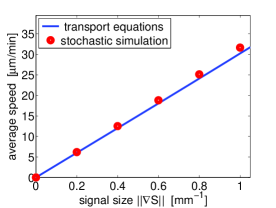
(a)   (b)

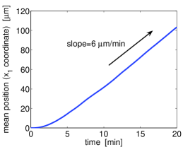
Figure 8: (a) Comparison of $\mathbf{v}_{av}^{\infty}$ computed by $(\ref{theoraverspeed})$ (solid curve) with results obtained by stochastic simulations (circles) for different values of $\parallel\!\!\nabla S\!\!\parallel$. (b) Average position of individuals (given by stochastic simulation) as a function of time for $\parallel\!\!\nabla S\!\!\parallel=0.2\;\mbox{\rm mm}^{-1}$.

shows $\mathbf{v}_{av}^{\infty}$ as a function of $\parallel\!\!\nabla S\!\!\parallel$.

The theoretical result (90) can be verified by stochastic simulations, and to that end we consider an ensemble of 500 cells. We discretize the boundary (36) of each cell using $m=50$ mesh points. Hence, the state of each cell is described by 54-dimensional vector (46) similarly as in Section 2.4. The internal dynamics model $\mathbf{y}$ written in terms of (19) is given by (36) – (37). The radius of a cell is set to $d=7.5\;\mu$m and we use parameter values (47) – (48) with $b=1\;\mbox{min}^{-1}$ and $\gamma=0.08\;\mbox{mm}^{2}$/min. The initial conditions are the same for all cells: namely all cells begin at position $\mathbf{x}={\mathbf{0}}$, their initial velocities satisfy $\mathbf{v}={\mathbf{0}}$, their internal variables are equal to $0$ around the entire membrane, and cells are initially unpolarized. The average position of cells as a function of time is given in Figure 8(b) for $\parallel\!\!\nabla S\!\!\parallel=0.2\;\mbox{\rm mm}^{-1}$. Since cells are initially unpolarized and resting, the initial cellular flux is zero. If we wait for a sufficiently long time, the average speed of the cells relaxes to a constant, and when we estimate this from long-time simulations, we obtain the values which are shown as circles in Figure 8(a). Comparing data in Figure 8(a), we see that the theoretical result (90) gives a very good approximation of the mean asymptotic speed estimated from simulations. This demonstrates the fact that one can extract population level information from the moment equations derived earlier.

Finally, we note that the previous analysis can be repeated for (85). The difference between (80) and (85) is the additional noise in the latter, which leads to the system (85). However, this noise will only influence the diffusion constant and the average speed of the population will be unchanged.

3.2 Further reduction of moment equations

One can further reduce the size of the system of moment equations (80) by supposing that the internal dynamics evolve much faster than changes in cytoskeleton and movement. Considering the excitation time $\tau_{e}=0$ and that the adaptation time $\tau_{a}\ll\tau_{d}$, we can assume the quasi-equilibrium in the equations for $\mathbf{n}_{\mathbf{q}}$ and $\mathbf{n}_{z}$ in (80), i. e.,

$$\mathbf{n}_{z}=\tau_{a}\left(\mathbf{I}_{3}-\tau_{a}\boldsymbol{\Lambda}\right)^{-1}\left[\dfrac{\partial S}{\partial t}\,\mathbf{n}+\left\{(\nabla S)^{T}\otimes{\bf J}\right\}\,\mathbf{j}\right]$$ (91)

and

$$\mathbf{n}_{\mathbf{q}}=\left[\mathbf{I}_{2}\otimes\left(\mathbf{I}_{3}-\tau_{a}\boldsymbol{\Lambda}\right)\right]^{-1}\left[\nabla S\otimes\mathbf{n}\right]$$ (92)

Substituting formulas (91) – (92) into (80), we can formally derive the reduced system of 7 moment equations for $\mathbf{n}$ and $\mathbf{j}$ only. These equations are derived under the assumption that $\tau_{a}$ is small. Passing formally to the limit $\tau_{a}\to 0$ in (91) – (92), we obtain $\mathbf{n}_{z}\to 0$ and $\mathbf{n}_{\mathbf{q}}\to\nabla S\otimes\mathbf{n}.$ As one would expect in light of the discussion following (45), the reduced equations predict movement up a steady gradient, but not in a periodic wave for $\tau_{a}=0$.

Another approach to eliminate the internal dynamics is to assume the quasi-equilibrium assumption directly in (43) – (44), i.e.

$$\mathbf{q}(\mathbf{x},t)\approx\nabla S(\mathbf{x},t)\qquad\mbox{and}\qquad z_{1}(\mathbf{x},t)\approx\tau_{a}\dfrac{\partial S}{\partial t}(\mathbf{x},t)+\tau_{a}\mathbf{v}\cdot\nabla S(\mathbf{x},t).$$

Denoting $p^{1}(\mathbf{x},\mathbf{v})$ the density of motile cells at position $\mathbf{x}\in\mathbb{R}^{2}$ with velocity $\mathbf{v}\in V\subset\mathbb{R}^{2}$, $p^{2}(\mathbf{x},\mathbf{v})$ the density of resting polarized cells at position $\mathbf{x}$ with polarization axis $\mathbf{v}$ and $n^{3}(\mathbf{x})$ the density of resting unpolarized cells, we can write transport equation for $p^{1},$ $p^{2}$ and $n^{3}$. Again 7 moment equations for $\mathbf{n}$ and $\mathbf{j}$ can be derived. Such equations were derived and analysed for one-dimensional case in Erban:2005:ICB . It was shown that in some parameter regimes, the reduced system approximates the simulation with a reasonable precision. See Erban:2005:ICB for details. The precision of the approximation depends on the parameter values chosen.

Finally one can ask whether the method developed in Erban:2004:ICB ; Erban:2005:STS , for reducing a hyperbolic system similar to (80) to the classical chemotaxis equations, can be applied here as well. In the context of chemotaxis based on a “run-and-tumble” strategy we were able to analytically compute the eigenvalues and eigenvectors of $\mathbf{A}(\mathbf{x},t)$, and it was shown that they are independent of the chemotactic signal. By exploiting the facts that the spectral gaps are signal-independent, and that reasonably simple formulas for eigenvectors are available, we reduced the hyperbolic system of moment equations to the classical chemotaxis description in the bacterial case Erban:2004:ICB ; Erban:2005:STS . In the case of system (80), the resulting slow eigenvalues are, for general values of parameters, very complicated functions of the parameters, and in particular they depend on the signal. To illustrate this, we consider the linear signal distribution (5) that leads to (89), we consider parameters from Section 3.1 and plot the real parts of the eigenvalues of $\mathbf{A}(\parallel\!\!\nabla S\!\!\parallel)$ as functions of $\parallel\!\!\nabla S\!\!\parallel$ in Figure 9. One sees there that the eigenvalues vary significantly with the signal strength.

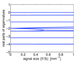
(a)   (b)

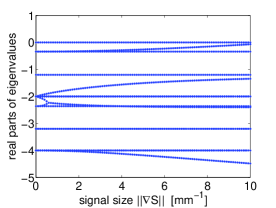
Figure 9: The real parts of the eigenvalues of $\mathbf{A}(\parallel\!\!\nabla S\!\!\parallel)$ for   (a) $\parallel\!\!\nabla S\!\!\parallel\in[0,1]\;\mbox{mm}^{-1};$ (b) $\parallel\!\!\nabla S\!\!\parallel\in[0,10]\;\mbox{mm}^{-1}.$

Further analysis is needed to better define the conditions under which the hyperbolic system can be reduced further. In that vein, we note that ignoring the term $\sum_{i=1}^{2}(\nabla S)_{i}j^{1}_{v_{i}}$ in equation (70) leads to the matrix $\mathbf{A}(\parallel\!\!\nabla S\!\!\parallel)$ which has signal-independent eigenvalues. Thus the possibility of further reduction clearly depends on the closure assumptions.

4 Discussion and conclusions

The goal in this paper was to derive macroscopic equations for the collective behavior of amoeboid cells based on models for individual-level behavior. In previous work we developed a moment closure approach to the transport equation for a velocity jump process that describes cell motion for cells that use a “run-and-tumble” strategy Erban:2004:ICB ; Erban:2005:STS . Here we demonstrated that this approach can also be applied to the more complex processes involved in the movement of crawling cells, and showed that one can predict important macroscopic characteristics from knowledge of the individual-level properties of these cells. We focused on chemotaxis in Dd as the model system because much is known about this system, but the general approach can be applied to any type of extracellular signal, including those that arise from all receptor-based interactions of a cell with its environment. Here we summarize the approach and discuss its advantages and limitations.

In Section 2 we introduced the general model (19) – (20) for the behavior of an individual eukaryotic cell. Since this model is often infinite-dimensional, we have to first reduce it to the finite-dimensional form (22) – (23). If such a reduction is possible, we can apply the transport equation framework (24) for the reduced set of variables. In this case we can derive the appropriate moment equations (80) and use them to study the macroscopic collective properties of cells, as we illustrated in Section 3.1 where we studied the dependence of the average speed of the cellular population on the strength of the extracellular signal.

Therefore the crucial assumption for a model which can be treated in the framework developed here is that the projection ${\cal P}$ from (21) exists and the equations (22) – (23) can be easily written. If this is not the case, it may be still possible to reduce the individual-level dynamics to a low-dimensional description of an individual cell. The behavior of these coarse (intracellular) observables (on the level of a cell) can be studied by computational equation-free methods which are currently being developed Kevrekidis:2003:EFM ; Erban:2006:GRN . The similar computational methods can be then used to study the population-level properties of the amoeboid cells using either the full model of an individual cell or the best available reduction of it Kevrekidis:2003:EFM ; Erban:2006:EFC .

The moment closure reduction of the transport equation used here can be justified for small signal gradients Erban:2004:ICB , but in the case of large signal gradients, the higher order moments may not be negligible and cannot be discarded. Similar moment methods can be used for any model assuming that the internal dynamics is close to its quasi-equilibrium. If the original internal dynamics model is nonlinear, it can be linearized around its equilibrium value for small signal gradients and the moment approach can be applied. Hence, the reader should view our linear model as an example of the linearization of more complex nonlinear problems. Of course, the linear model is clearly not valid for large signal gradients, but this is not the parameter regime studied in this paper. However, even some strongly-nonlinear models for internal dynamics produce simple input-output behavior that can be captured by a linear model with possibly signal-dependent parameters Erban:2005:STS , and thus the results presented here may have broader applicability than the deriviation would suggest if applied strictly.

In the case of a constant external signal gradient we were able to derive explicit expressions for various statistics of the motion from the hyperbolic system derived from the transport equation. We also discussed the predicted behavior of models for experimental conditions such as spatio-temporal waves of chemoattractant. It is known that eukaryotic cells such as Dd or leukocytes aggregate at the source of the waves, and the models studied here include the processes, such as adaptation, that are necessary to reproduce this behavior.

The models described here are all based on deterministic extracellular signals, although a small random component was added to the choice of direction. The effects of stochastic fluctuations in signal detection and processing on movement were introduced in Dickinson:1995:TEI , where stochastic differential equations are postulated to model cell movement on the time scale of the molecular processes that govern locomotion. Some concrete estimates of the probable role of noise in the signal seen be a Dd cell were made in Othmer:1998:OCS . However a much more detailed analysis of stochastic effects in all components of the movement response is needed.

- (1) W. Alt, Biased random walk models for chemotaxis and related diffusion approximations, Journal of Mathematical Biology 9 (1980), 147–177.
- (2) N. Barkai and S. Leibler, Robustness in simple biochemical networks, Nature 387 (1997), 913–917.
- (3) H. Berg, How bacteria swim, Scientific American 233 (1975), 36–44.
- (4) H. Berg and D. Brown, Chemotaxis in Esterichia coli analysed by three-dimensional tracking, Nature 239 (1972), 500–504.
- (5) R. Bourret and A. Stock, Molecular information processing: lessons from bacterial chemotaxis, Journal of Biological Chemistry 277 (2002), no. 12, 9625–9628.
- (6) F. Chalub, P. Markowich, B. Perthame, and C. Schmeiser, Kinetic models for chemotaxis and their drift-diffusion limits, Monatshefte für Mathematik 142 (2004), no. 1-2, 123–141.
- (7) C. Chung, S. Funamoto, and R. Firtel, Signaling pathways controlling cell polarity and chemotaxis, Trends in Biochemical Sciences 26 (2001), no. 9, 557–566.
- (8) J. Condeelis, A. Bresnick, M. Demma, S. Dharmawardhane, R. Eddy, A. Hall, R. Sauterer, and V. Warrenand, Mechanisms of ameboid chemotaxis: An evaluation of the cortical expansion model, Developmental Genetics 11 (1990), no. 5-6, 333–340.
- (9) J. Dallon and H. Othmer, A discrete cell model with adaptive signalling for aggregation of dictyostelium discoideum, Philosophical Transactions of the Royal Society B: Biological Sciences 352 (1997), no. 1351, 391–417.
- (10) , A continuum analysis of the chemotatic signal seen by dictyostelium discoideum, Journal of Theoretical Biology 194 (1998), no. 4, 461–483.
- (11) R. Dickinson and R. Tranquillo, Transport equations and indices for random and biased cell migration based on single cell properties, SIAM Journal on Applied Mathematics 55 (1995), 1419–1454.
- (12) Y. Dolak and C. Schmeiser, Kinetic models for chemotaxis: Hydrodynamic limits and spatio-temporal mechanisms, Journal of Mathematical Biology 51 (2005), no. 6, 595 – 615.
- (13) R. Erban, From individual to collective behaviour in biological systems, Ph.D. thesis, University of Minnesota, 2005.
- (14) R. Erban and H. Hwang, Global existence results for the complex hyperbolic models of bacterial chemotaxis, submitted to Discrete and Continuous Dynamical Systems Series B, available as Preprint 118/2005, www.mis.mpg.de/preprints, 2006.
- (15) R. Erban, I. Kevrekidis, D. Adalsteinsson, and T. Elston, Gene regulatory networks: A coarse-grained, equation-free approach to multiscale computation, to appear in Journal of Chemical Physics, 30 pages, 2006.
- (16) R. Erban, I. Kevrekidis, and H. Othmer, An equation-free computational approach for extracting population-level behavior from individual-based models of biological dispersal, to appear in Physica D, 30 pages, available as http://arxiv.org/physics/0505179, 2006.
- (17) R. Erban and H. Othmer, From individual to collective behaviour in bacterial chemotaxis, SIAM Journal on Applied Mathematics 65 (2004), no. 2, 361–391.
- (18) , From signal transduction to spatial pattern formation in E. coli: A paradigm for multi-scale modeling in biology, Multiscale Modeling and Simulation 3 (2005), no. 2, 362–394.
- (19) P. Fisher, R. Merkl, and G. Gerisch, Quantitative analysis of cell motility and chemotaxis in Dictyostelium discoideum by using an image processing system and a novel chemotaxis chamber providing stationary chemical gradients, Journal of Cell Biology 108 (1989), 973–984.
- (20) R. Ford and D. Lauffenburger, A simple expression for quantifying bacterial chemotaxis using capillary assay data: Application to the analysis of enhanced chemotactic responses from growth-limited cultures, Mathematical Biosciences 109 (1992), no. 2, 127–150.
- (21) J. Geiger, D. Wessels, and D. Soll, Human polymorphonuclear leukocytes respond to waves of chemoattractant, like dictyostelium, Cell Motility and the Cytoskeleton 56 (2003), 27–44.
- (22) G. Gerisch, Chemotaxis in Dictyostelium, Annual Review of Physiology 44 (1982), 535–552.
- (23) G. Gerisch, H. Fromm, A. Huesgen, and U. Wick, Control of cell-contact sites by cyclic AMP pulses in differentiating Dictyostelium cells, Nature 255 (1975), 547–549.
- (24) T. Hillen and H. Othmer, The diffusion limit of transport equation derived from velocity-jump processes, SIAM Journal on Applied Mathematics 61 (2000), 751–775.
- (25) T. Höfer and P. Maini, Streaming instability of slime mold amoebae: An analytical model, Physical Review E 56 (1997), no. 2, 1–7.
- (26) M. Iijima, Y.E. Huang, and P. Devreotes, Temporal and spatial regulation of chemotaxis, Developmental Cell 3 (2002), 469–478.
- (27) T. Jin, N. Zhang, Y. Long, C. Parent, and P. Devreotes, Localization of the G protein complex in living cells during chemotaxis, Science 287 (2000), 1034–1036.
- (28) E. Keller and L. Segel, Initiation of slime mold aggregation viewed as an instability, Journal of Theoretical Biology 26 (1970), 399–415.
- (29) I. Kevrekidis, C. Gear, J. Hyman, P. Kevrekidis, O. Runborg, and K. Theodoropoulos, Equation-free, coarse-grained multiscale computation: enabling microscopic simulators to perform system-level analysis, Communications in Mathematical Sciences 1 (2003), no. 4, 715–762.
- (30) D. Koshland, Bacterial chemotaxis as a model behavioral system, New York: Raven Press, 1980.
- (31) J. Krishnan and P. Iglesias, A modelling framework describing the enzyme regulation of membrane lipids underlying gradient perception in Dictyostelium cells II: input-output analysis, Journal of Theoretical Biology 235 (2005), 504–520.
- (32) B. Lilly, J. Dallon, and H. Othmer, Pattern formation in a cellular slime mold, Numerical methods for bifurcation problems and large-scale dynamical systems (E. Doedel and L. Tuckerman, eds.), Springer-Verlag, New York, 2000, IMA proceedings, vol. 119, pp. 359–383.
- (33) J. Martiel and A. Goldbeter, A model based on receptor desensitization for cyclic AMP signaling in Dictyostelium cells, Biophysical Journal 52 (1987), 807–828.
- (34) J. Mato, A. Losada, V. Nanjundiah, and T. Konijn, Signal input for a chemotactic response in the cellular slime mold Dictyostelium discoideum, Proceedings of the National Academy of Sciences USA 72 (1975), 4991–4993.
- (35) H. Meinhardt, Orientation of chemotactic cells and growth cones: models and mechanisms, Journal of Cell Science 112 (1999), 2867–2874.
- (36) T. Mitchison and L. Cramer, Actin-based cell motility and cell locomotion, Cell 3 (1996), 371–379.
- (37) H. Othmer, S. Dunbar, and W Alt, Models of dispersal in biological systems, Journal of Mathematical Biology 26 (1988), 263–298.
- (38) H. Othmer and T. Hillen, The diffusion limit of transport equations 2: Chemotaxis equations, SIAM Journal on Applied Mathematics 62 (2002), 1222–1250.
- (39) H. Othmer and P. Schaap, Oscillatory cAMP signaling in the development of Dictyostelium discoideum, Comments on Theoretical Biology 5 (1998), 175–282.
- (40) C. Parent and P. Devreotes, A cell’s sense of direction, Science 284 (1999), 765–770.
- (41) E. Pate and H. Othmer, Differentiation, cell sorting and proportion regulation in the slug stage of Dictyostelium discoideum, Journal of Theoretical Biology 118 (1986), 301–319.
- (42) C. Patlak, Random walk with persistence and external bias, Bulletin of Mathematical Biophysics 15 (1953), 311–338.
- (43) M. Sheetz, D. Felsenfeld, C. Galbraith, and D. Choquet, Cell migration as a five-step cycle, Biochemical Society Symposia 65 (1999), 233–243.
- (44) D. Soll, The use of computers in understanding how animal cells crawl, International Review of Cytology (K. Jeon and J. Jarvik, eds.), vol. 163, Academic Press, 1995, pp. 43–104.
- (45) P. Sperb, On a mathematical model describing the aggregation of amoebae, Bulletin of Mathematical Biology 41 (1979), 555–572.
- (46) P. Spiro, J Parkinson, and H. Othmer, A model of excitation and adaptation in bacterial chemotaxis, Proceedings of the National Academy of Sciences USA 94 (1997), 7263–7268.
- (47) J. Swanson and D. Taylor, Local and spatially coordinated movements in Dictyostelium discoideum amoebae during chemotaxis, Cell 28 (1982), 225–232.
- (48) Y. Tang and H. Othmer, A G protein-based model of adaptation in Dictyostelium discoideum, Mathematical Biosciences 120 (1994), no. 1, 25–76.
- (49) , Excitation, oscillations, and wave propagation in Dictyostelium discoideum, Philosophical Transactions of the Royal Society B: Biological Sciences (1995), 179–195.
- (50) R. Tranquillo and D. Lauffenburger, Stochastic model of leukocyte chemosensory movement, Journal of Mathematical Biology 25 (1987), no. 3, 229 – 262.
- (51) B. Varnum-Finney, E. Voss, and D. Soll, Frequency and orientation of pseudopod formation of Dictyostelium discoideum amoebae chemotaxing in a spatial gradient: Further evidence for a temporal mechanism, Cell Motility and the Cytoskeleton 8 (1987), no. 1, 18–26.
- (52) R. Weis and D. Koshland, Reversible receptor methylation is essential for normal chemotaxis of Escherichia coli in gradients of aspartic acid, Proceedings of the National Academy of Sciences USA 85 (1988), 83–87.
- (53) D. Wessels, J. Murray, and D. Soll, Behavior of Dictyostelium amoebae is regulated primarily by the temporal dynamic of the natural cAMP wave, Cell Motility and the Cytoskeleton 23 (1992), no. 2, 145–156.
- (54) D. Wessels, H. Zhang, J. Reynolds, K. Daniels, P. Heid, S. Lu, A. Kuspa, G. Shaulsky, W. Loomis, and D. Soll, The internal phosphodiesterase RegA is essential for the suppression of lateral pseudopods during Dictyostelium chemotaxis, Molecular Biology of the Cell 11 (2000), no. 8, 2803–2820.