Complex collective states in a one-dimensional two-atom system

Abstract

We consider a pair of identical two-level atoms interacting with a scalar field in one dimension, separated by a distance $x_{21}$. We restrict our attention to states where one atom is excited and the other is in the ground state, in symmetric or anti-symmetric combinations. We obtain exact collective decaying states, belonging to a complex spectral representation of the Hamiltonian. The imaginary parts of the eigenvalues give the decay rates, and the real parts give the average energy of the collective states. In one dimension there is strong interference between the fields emitted by the atoms, leading to long-range cooperative effects. The decay rates and the energy oscillate with the distance $x_{21}$. Depending on $x_{21}$, the decay rates will either decrease, vanish or increase as compared with the one-atom decay rate. We have sub- and super-radiance at periodic intervals. Our model may be used to study two-cavity electron wave-guides. The vanishing of the collective decay rates then suggests the possibility of obtaining stable configurations, where an electron is trapped inside the two cavities.

I Introduction

Systems of interacting atoms form collective states where the atoms behave differently from isolated ones Dicke ; Woger . For atoms in their ground states the collective effects are relatively small. They produce the van-der Waals or Casimir-Polder forces between atoms Compagno , associated with the cloud of virtual photons surrounding the atoms.

When the atoms are in excited states they can exchange real photons originated by spontaneous emission. Depending on the situation, the real photons can give strong collective effects, altering the forces between atoms and also their rate of spontaneous emission Dicke ; Stephen ; Milonni . For example for identical atoms in three dimensions separated by small distances, the decay rate will essentially double or vanish, depending on whether the initial state is symmetric or antisymmetric with respect to exchange of atoms Stephen ; Dung . We have “super-radiance” or “sub-radiance,” respectively. If the atoms are not identical Power , or if the distance between the atoms is larger than their characteristic wavelengths, the effects become much smaller Stephen .

Most studies on two-atoms (see, e.g., Refs. Dicke ; Woger ; Compagno ; Stephen ; Milonni ; Dung ; Power ; Dung2 ; Kweon ; Ficek ) focus on three-dimensional systems. In this paper we will consider a one-dimensional system. We will show that the exchange of real photons gives strong collective effects even for large separations between the atoms.

Our system is analogous to electron wave guides consisting of two cavities connected by a lead Suresh0 ; Suresh . Hence the effects we will discuss may be studied experimentally.

We will consider a simplified model where we have two identical two-level atoms, with basis states where one atom is excited, while the other is in the ground state. We will use the dipole and rotating-wave approximations for the interaction with the field.

We will describe the collective two-atom states through complex eigenstates of the Hamiltonian Nakanishi ; Sudarshan ; Bohm ; PPT . The complex eigenstates decay exponentially in time, breaking time-symmetry. The real and imaginary parts of the complex eigenvalues give the average energy of the collective states and the emission rates, respectively.

The Hamiltonian, being a Hermitian operator, can only have complex eigenvalues if the eigenstates do not belong to a Hilbert space. In one-atom systems the non-Hilbertian nature of the complex states is manifested in their field intensity, which includes a factor growing exponentially with the distance from the atom. This growth in space is related to the exponential decay of the atom in time POP2001 . The exponential field inside the light-cone of the atom represents the real emitted photons. As we will show, this field has physical effects, which can be seen adding a second atom.

Outside the light-cone, the field associated with the complex eigenstates grows exponentially without truncation. However, including the complete set of eigenstates in the complex representation of the Hamiltonian, the exponential field outside the light-cone is cancelled by renormalized field states POP2001 . This is consistent with causality, because the field further away from the atom is emitted earlier. Going further away, one reaches the point corresponding to the time where the atom was excited. At this point the field stops growing.

One can introduce complex states that are truncated outside the light-cone, using distributions dependent on the test functions or observables. These are considered in Ref. Sungyun .

In the two-atom system, the real photons emitted by each atom are absorbed by the other atom. In $d$ dimensions the emitted field includes a $1/r^{d-1}$ decrease factor with distance. Hence the field has a strong effect in $d=1$ dimensions, as compared with $d=2$ or $3$ dimensions.

We will show that in one dimension the decay rates of the collective states oscillate with the distance between the atoms. In contrast to Dicke’s states Dicke , both symmetric and antisymmetric states of the two atoms can become sub-radiant and super-radiant as the distance between the two atoms is varied. For distances that are integer multiples of the atom wavelength, the collective decay rates vanish, leading to stable collective states. These states can trap field energy between the atoms.

In Sec. II we briefly discuss the complex representation of the Hamiltonian for a one-atom system. In Sec. III we introduce our two-atom model and its complex collective eigenstates. In Secs. IV and V we discuss the emergence of the collective states and the bouncing of photons between the atoms. In Sec. VI we consider the decay rate and average energy of the collective states as a function of the distance between the atoms. We discuss super-radiance and sub-radiance, including stable collective states mentioned above. We also give a heuristic discussion on the force between the atoms. In Sec. VII we discuss the mapping of our model to a two-cavity electron wave guide, and show that this system allows an approximate stable collective state.

II One-atom system

In order to introduce the complex spectral representation of the Hamiltonian, we consider first a single two-level atom interacting with a field in one-dimensional space. This is the Friedrichs-Lee model in one dimension. We briefly review the main results. More details can be found in Ref. PPT .

The Hamiltonian is given by

$$H = {H}_{0}\ +\lambda V$$

$$= \omega_{1}|1\rangle\langle 1|+\sum\limits_{k}\omega_{k}|k\rangle\langle k|+\lambda\sum\limits_{k}V_{k}(|k\rangle\langle 1|+|1\rangle\langle k|).$$

where we put $c=\hbar=1$. The state $|1\rangle$ represents the bare atom in its excited level with no field present, while the state $|k\rangle$ represents a bare field mode (“photon”) of momentum $k$ together with the atom in its ground state (see Figure 1).

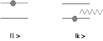
Figure 1: One-atom system

The energy of the ground state is chosen to be zero; $\omega_{1}$ is the bare energy of the excited level and $\omega_{k}\equiv|k|$ is the photon energy. The coupling constant $\lambda\ll 1$ is dimensionless. We assume periodic boundary conditions. We put the system in a “box” of size $L$ and take the limit $L\to\infty$. For $L$ finite the momenta $k$ are discrete. In the limit $L\to\infty$ they become continuous, i.e.,

$${2\pi\over L}\sum_{k}\to\int dk.$$ (2)

We have $\langle a|b\rangle=\delta_{a,b}=$ Kroenecker delta. In the limit $L\to\infty$,

$${L\over 2\pi}\delta_{k,k^{\prime}}\to\delta(k-k^{\prime}).$$ (3)

The interaction term is obtained through the dipole approximation as well as the rotating-wave approximation. The potential $V_{k}$ is of order $L^{-1/2}$. For convenience we write

$$V_{k}=(2\pi/L)^{1/2}v_{k},$$ (4)

where $v_{k}$ is of order $1$ in the continuous spectrum limit $L\to\infty$. As a specific example we will assume that Drude ; FP99

$$v_{k}=v(\omega_{k})={\omega_{k}^{1/2}\over[1+(\omega_{k}/\omega_{M})^{2}]^{n}}$$ (5)

with $n=1$. The constant $\omega_{M}^{-1}$ determines the range of the interaction. We shall assume that the interaction is of short range, i.e., $\omega_{M}\gg\omega_{1}$.

The state $|1\rangle$ is unstable if

$$\omega_{1}>\int_{-\infty}^{\infty}dk\,\frac{\lambda^{2}v_{k}^{2}}{\omega_{k}}$$ (6)

Otherwise, it is stable cohen . Hereafter we will consider the unstable case.

In the unstable case one can construct renormalized field eigenstates that diagonalize the Hamiltonian as

$$H=\sum_{k}|{\tilde{\phi}}_{k}^{\pm}\rangle\omega_{k}\langle{\tilde{\phi}}_{k}^{\pm}|$$ (7)

where

$$\lim_{\lambda\to 0}|{\tilde{\phi}}_{k}^{\pm}\rangle=|k\rangle$$ (8)

and hereafter we use the summation over field modes in the sense of Eq. (2). The index $\pm$ refers to either “in” or “out” scattering eigenstates.

The explicit form of the eigenstates is given by PPT

$$|{\tilde{\phi}}_{k}^{\pm}\rangle=|k\rangle+{\lambda V_{k}\over\eta^{\pm}(\omega_{k})}\left[|1\rangle+{\sum_{l}}{\lambda V_{l}\over\omega_{k}-\omega_{l}\pm i\epsilon}|l\rangle\right]$$ (9)

where $\epsilon$ is an infinitesimal positive number. The limit $\epsilon\to 0$ is taken after the limit $L\to\infty$. In Eq. (9),

$$\eta^{\pm}(\omega) \equiv \omega-\omega_{1}-\sum_{k^{\prime}}{\lambda^{2}V_{k^{\prime}}^{2}\over(\omega-\omega_{k^{\prime}})^{\pm}}$$ (10)

$$= \omega-\omega_{1}-2\int_{0}^{\infty}dk^{\prime}\,{\lambda^{2}v_{k^{\prime}}^{2}\over(\omega-k^{\prime})^{\pm}}$$

is the inverse of Green’s function. The $+$ (or $-$) superscript in Eq. (10) indicates analytic continuation from the upper (or lower) half-plane of $\omega$ PPT . Using the complex delta-function $\delta_{C}$ Nakanishi we can write

$$\frac{1}{(\omega-k^{\prime})^{\pm}}=\left\{\begin{array}[]{ll}(\omega-k^{\prime})^{-1},&\pm{\rm Im\,}\omega>0\\ (\omega-k^{\prime})^{-1}\mp 2\pi i\delta_{C}(k^{\prime}-\omega),&\pm{\rm Im\,}\omega<0\end{array}\right.$$ (13)

(14)

When $\omega$ is real, we have

$$\eta^{\pm}(\omega)\equiv\omega-\omega_{1}-2\int_{0}^{\infty}dk^{\prime}\frac{\lambda^{2}v_{k^{\prime}}^{2}}{\omega-k^{\prime}\pm i\epsilon}.$$ (15)

With our form factor and small $\lambda$, Green’s function has one pole $z_{1}$ in the lower half plane, i.e., $\eta^{+}(z_{1})=0$ for

$$z_{1}\equiv{\tilde{\omega}}_{1}-i\gamma_{1}$$ (16)

The negative imaginary part $-i\gamma_{1}$ describes decay for $t>0$. The real part ${\tilde{\omega}}_{1}$ gives the shifted average energy of the excited state. For the other branch we have $\eta^{-}(z_{1}^{*})=0$, with $z_{1}^{*}$ describing decay for $t<0$.

Note that in the representation (7) the decay rate and shifted energy of the excited state do not appear in the spectrum. One can incorporate $z_{1}$ (or $z_{1}^{*}$) into the spectrum by extracting the residue of Eq. (7) at the pole $\omega_{k}=z_{1}$ (or $z_{1}^{*}$). This gives the complex spectral decompositions PPT ; Nakanishi ; Sudarshan ; Bohm :

$$H = |\phi_{1}\rangle z_{1}\langle{\tilde{\phi}}_{1}|+\sum_{k}|\phi_{k}^{+}\rangle\omega_{k}\langle{\tilde{\phi}}_{k}^{+}|$$ (17)

$$= |{\tilde{\phi}}_{1}\rangle z_{1}^{*}\langle\phi_{1}|+\sum_{k}|\phi_{k}^{-}\rangle\omega_{k}\langle{\tilde{\phi}}_{k}^{-}|$$

The state $|\phi_{1}\rangle$ and its dual $\langle{\tilde{\phi}}_{1}|$ are complex eigenstates of $H$. Their explicit forms are PPT

$$|\phi_{1}\rangle=N_{1}^{1/2}\Big{[}|1\rangle+\sum_{k}|k\rangle{\lambda V_{k}\over(z_{1}-\omega_{k})^{+}}\Big{]},$$ (18)

$$|{\tilde{\phi}}_{1}\rangle=[N_{1}^{*}]^{1/2}\Big{[}|1\rangle+\sum_{k}|k\rangle{\lambda V_{k}\over(z_{1}^{*}-\omega_{k})^{-}}\Big{]}.$$

The state $|\phi_{k}^{+}\rangle$ has the same form as the state $|{\tilde{\phi}}_{k}^{+}\rangle$ with the replacement

$$\frac{1}{\eta^{+}(\omega_{k})}\Rightarrow\frac{1}{\eta^{+}(\omega_{k})}\frac{\omega_{k}-z_{1}}{(\omega_{k}-z_{1})^{+}}$$ (19)

and similarly, the state $|\phi_{k}^{-}\rangle$ has the same form as the state $|{\tilde{\phi}}_{k}^{-}\rangle$ with the complex conjugate replacement.

The states in Eq. (17) form a bi-orthormal set, with the relations

$$\langle{\tilde{\phi}}_{1}|\phi_{1}\rangle=1,\;\;\langle{\tilde{\phi}}_{k}^{+}|\phi_{1}\rangle=0$$

$$\langle{\tilde{\phi}}_{k}^{+}|\phi_{k^{\prime}}^{+}\rangle=\delta_{k,k^{\prime}}$$ (20)

and their complex-conjugate relations.

III Two-atom system

In this Section we discuss the complex spectral representation of a two-atom system with Hamiltonian

$$H = \omega_{1}|1\rangle\langle 1|+\omega_{2}|2\rangle\langle 2|+\sum_{k}\omega_{k}|k\rangle\langle k|$$ (21)

$$+ \sum_{k}\lambda_{1}V_{k}\left(e^{ikx_{1}}|1\rangle\langle k|+e^{-ikx_{1}}|k\rangle\langle 1|\right)$$

$$+ \sum_{k}\lambda_{2}V_{k}\left(e^{ikx_{2}}|2\rangle\langle k|+e^{-ikx_{2}}|k\rangle\langle 2|\right)$$

The state $|1\rangle$ represents atom 1 in its excited state, while atom 2 is in the ground state and no field is present. Conversely, the state $|2\rangle$ represents atom 2 in its excited state, while atom 1 is in the ground state and no field is present. The state $|k\rangle$ represents a field mode $k$ with both atom 1 and atom 2 are in their ground states (see Figure 2). The atoms 1 and 2 are located at the positions $x_{1}$ and $x_{2}$, respectively. We use the potential in Eq. (5).

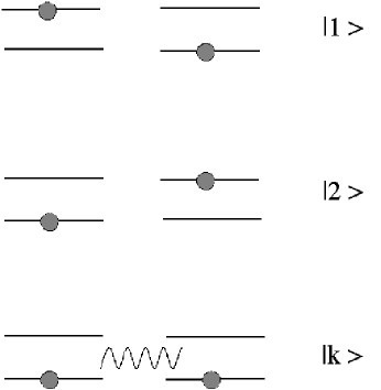
Figure 2: Two-atom system

We will first assume that the two atoms are at fixed positions, so that the distance between them

$$x_{21}=|x_{2}-x_{1}|$$ (22)

is fixed. This can happen if the atoms are heavy. A system of two fixed atoms is analogous to a two-cavity waveguide (see Sec. VII).

We will consider the case where the two atoms are identical,

$$\lambda_{1}=\lambda_{2}=\lambda$$

$$\omega_{1}=\omega_{2}$$ (23)

We introduce the symmetric and antisymmetric states

$$|s\rangle=\frac{|1\rangle+|2\rangle}{\sqrt{2}},\qquad|a\rangle=\frac{|1\rangle-|2\rangle}{\sqrt{2}}$$ (24)

which are eigenstates of the unperturbed Hamiltonian $H_{0}=H(\lambda=0)$ as

$$H_{0}|j\rangle=\omega_{j}|j\rangle,\quad j=s,a$$ (25)

$$\omega_{s}=\omega_{a}=\omega_{1}.$$ (26)

We will use the notation

$$\sigma_{j}\equiv\left\{\begin{array}[]{ll}1,&\mbox{for $j=s$}\\ -1,&\mbox{for $j=a$,}\end{array}\right.$$ (29)

With this notation we have $|j\rangle=(|1\rangle+\sigma_{j}|2\rangle)/\sqrt{2}$.

As for the one-atom system, we can diagonalize the Hamiltonian as

$$H=\sum_{k}|{\tilde{F}}_{k}^{\pm}\rangle\omega_{k}\langle{\tilde{F}}_{k}^{\pm}|$$ (30)

where

$$|{\tilde{F}}_{k}^{\pm}\rangle=|k\rangle+\beta^{\pm}_{sk}|s\rangle+\beta^{\pm}_{ak}|a\rangle+\sum_{k^{\prime}}\beta^{\pm}_{k^{\prime}k}|k^{\prime}\rangle$$ (31)

and

$$\beta^{\pm}_{jk}=\frac{1}{\sqrt{2}}\frac{\lambda V_{k}}{\eta_{j}^{\pm}(\omega_{k})}\left(e^{ikx_{1}}+\sigma_{j}e^{ikx_{2}}\right)$$ (32)

$$\beta^{\pm}_{k^{\prime}k}=\frac{1}{\sqrt{2}}\frac{\lambda V_{k}}{\omega_{k}-\omega_{k^{\prime}}\pm i\epsilon}\sum_{j=s,a}\beta^{\pm}_{jk}\left(e^{-ik^{\prime}x_{1}}+\sigma_{j}e^{-ik^{\prime}x_{2}}\right)$$ (33)

$$\eta^{\pm}_{j}(\omega)$$

$$=\omega-\omega_{1}-2\int_{0}^{\infty}dk^{\prime}\frac{\lambda^{2}v_{k^{\prime}}^{2}}{(\omega-k^{\prime})^{\pm}}\left(1+\sigma_{j}\cos(k^{\prime}x_{21})\right)$$

(34)

Following a procedure similar to one found in Ref. PPT , one can show that the new diagonalized states $|{\tilde{F}}_{k}^{\pm}\rangle$ satisfy the orthogonality and completeness relations

$$\sum_{k}|{\tilde{F}}_{k}^{\pm}\rangle\langle{\tilde{F}}_{k}^{\pm}|=|1\rangle\langle 1|+|2\rangle\langle 2|+\sum_{k}|k\rangle\langle k|$$ (35)

$$\langle{\tilde{F}}_{k}^{+}|{\tilde{F}}_{k^{\prime}}^{+}\rangle=\langle{\tilde{F}}_{k}^{-}|{\tilde{F}}_{k^{\prime}}^{-}\rangle=\delta_{k,k^{\prime}}$$ (36)

Green’s function $[\eta^{+}_{j}(\omega)]^{-1}$ has poles in the lower half-plane, and conversely, $[\eta^{-}_{j}(\omega)]^{-1}$ has poles in the upper half-plane. From now on we discuss only the $+$ branch with poles on the lower half-plane.

A new feature with respect to the one-atom system is that due to the cosine term in Eq. (34), there are many poles of Green’s function, as shown in Fig. 3. We label the poles as

$$z_{j,n}={\tilde{\omega}}_{j,n}-i\gamma_{j,n}$$ (37)

where $n$ is an integer.

The poles $z_{j,n}$ are solutions of the equation

$$\eta^{+}_{j}(z_{j,n})=0$$ (38)

In the following we discuss this equation and its solutions.

From Eqs. (14) and (34) we obtain

$$z_{j,n} = \omega_{1}+2\int_{0}^{\infty}dk^{\prime}\frac{\lambda^{2}v_{k^{\prime}}^{2}}{z_{j,n}-k^{\prime}}\left(1+\sigma_{j}\cos(k^{\prime}x_{21})\right)$$ (39)

$$- 4\pi i\lambda^{2}[v_{z_{j,n}}]^{2}\left(1+\sigma_{j}\cos(z_{j,n}x_{21})\right)$$

Note that cosine in the last term includes the factor $\exp(\gamma_{j,n}x_{21})$, which grows exponentially with the distance $x_{21}$ between the atoms. Assuming weak coupling and taking only the pole contribution in the $k^{\prime}$ integral we obtain the set of equations

$${\tilde{\omega}}_{j,n}\approx\omega_{1}+2\pi[\lambda v({\tilde{\omega}}_{j,n})]^{2}\sigma_{j}e^{\gamma_{j,n}x_{21}}\sin({\tilde{\omega}}_{j,n}x_{21})$$ (40)

$$\gamma_{j,n}\approx 2\pi[\lambda v({\tilde{\omega}}_{j,n})]^{2}\left[1+\sigma_{j}e^{\gamma_{j,n}x_{21}}\cos({\tilde{\omega}}_{j,n}x_{21})\right]$$ (41)

In Fig. 3, the pole of $[\eta^{+}_{s}(\omega)]^{-1}$ with real part closest to the unperturbed frequency $\omega_{1}$ is also closest to the real axis. We call this pole $z_{s,0}=z_{s}$. Similarly, for $[\eta^{+}_{a}(\omega)]^{-1}$ we denote the pole closest to $\omega_{1}$ as $z_{a,0}=z_{a}$. Both these poles are obtained by a perturbation expansion around $\lambda=0$. We have

$$z_{j,0}=z_{j}\to\omega_{1}\quad{\rm as\,\,}\lambda\to 0.$$ (42)

If $x_{21}$ is not too large ($x_{21}\sim\gamma_{1}^{-1}$ or smaller), one can show that the poles $z_{j,n}$ are given by

$$z_{j,n}\approx\left\{\begin{array}[]{ll}z_{j}+2n\pi/x_{21}+\delta z_{j,n},&\mbox{for $\sigma_{j}n>0$}\\ z_{j}+(2n+\sigma_{j})\pi/x_{21}+\delta z_{j,n},&\mbox{for $\sigma_{j}n<0$.}\end{array}\right.$$ (45)

(46)

where $\delta z_{j,n}$ is an $O(\lambda^{2}$) correction. The approximate value ${\rm Re}(z_{j,n}-z_{j})$ predicted by this equation agrees with Fig. 3 (for $j=s$) and a similar figure for $j=a$, which we omit.

We write the poles $z_{j}$ as

$$z_{j}={\tilde{\omega}}_{j}-i\gamma_{j}.$$ (47)

The poles $z_{j}$, having the smallest decay rates $\gamma_{j}$, will give a dominant contribution to the time evolution after a few bounces of the field between the atoms. In this way, the complex collective states defined in Eq. (48) emerge.

As in the one-atom system we can obtain complex eigenstates $|\phi_{j}\rangle$ of the total Hamiltonian, such that

$$H|\phi_{j}\rangle=z_{j}|\phi_{j}\rangle$$ (48)

Figure 3: Contour plot of $\log(1/|\eta_{s}^{+}(z)|)$. The $x$ and $y$ axes are ${\rm Re}(z)$ and ${\rm Im}(z)$, respectively. The contours concentrate around the poles $z_{s,n}$ of Green’s function. Parameters are $x_{21}=29.025$, $\omega_{1}=2$, $\lambda=0.05$, $\omega_{M}=5$.

Their explicit forms are given by

$$|\phi_{j}\rangle$$

$$=N_{j}^{1/2}\left[|j\rangle+\sum_{k}\frac{2^{-1/2}\lambda V_{k}}{(z_{j}-\omega_{k})^{+}}\left(e^{-ikx_{1}}+\sigma_{j}e^{-ikx_{2}}\right)|k\rangle\right]$$

(49)

where

$$N_{j}=\left[1+\sum_{k}\frac{\lambda^{2}V_{k}^{2}}{[(z_{j}-\omega_{k})^{+}]^{2}}(1+\sigma_{j}\cos kx_{21})\right]^{-1}.$$ (50)

For these states we have $|\phi_{j}\rangle\rightarrow|j\rangle$ as $\lambda\rightarrow 0$.

The dual states satisfying $\langle{\tilde{\phi}}_{j}|H=z_{j}\langle{\tilde{\phi}}_{j}|$ are given by

$$\langle{\tilde{\phi}}_{j}|=N_{j}^{1/2}\left[\langle j|+\sum_{k}\frac{2^{-1/2}\lambda V_{k}}{(z_{j}-\omega_{k})^{+}}\left(e^{ikx_{1}}+\sigma_{j}e^{ikx_{2}}\right)\langle k|\right]$$

(51)

Like in the one-atom case, we have the complex spectral representation

$$H=\sum_{j=s,a}|\phi_{j}\rangle z_{j}\langle{\tilde{\phi}}_{j}|+\sum_{k}|F_{k}^{+}\rangle\omega_{k}\langle{\tilde{F}}_{k}^{+}|$$ (52)

where $|F_{k}^{+}\rangle$ has the same form as the state $|{\tilde{F}}_{k}^{+}\rangle$ with the replacement

$$\frac{1}{\eta^{+}_{j}(\omega_{k})}\Rightarrow\frac{1}{\eta^{+}_{j}(\omega_{k})}\frac{\omega_{k}-z_{j}}{(\omega_{k}-z_{j})^{+}}$$ (53)

We have as well the complex-conjugate representation, taking the complex-conjugates of Eqs. (52), (53).

IV Emergence of the complex collective states

Time evolution of the two atom system can be solved by using Eq. (30) or Eq. (52). As an example we assume the atoms are initially in the symmetric state $|s\rangle$ and the initial field is zero (similar calculations can be done if the initial state is $|a\rangle$). We will calculate the survival probability of state $|1\rangle$,

$$P_{1}(t)=|\langle 1|e^{-iHt}|s\rangle|^{2}$$ (54)

Before we go into details, we can guess the behavior the system will show. Since the initial state is symmetric, the following discussion also applies with atoms 1 and 2 exchanged. Say atom 1 is to the left of atom 2. At the beginning, atom 1 decays and emits a field. Half of this field will be radiated away to the left, while the other half will reach and excite atom 2. Atom 2 will then decay and emit its own field, part of which will be radiated away to the right, the rest going to the left, back towards atom 1. Continuing this process, we see that energy will bounce back and forth between the two atoms. As time passes, this energy will decrease due to the outgoing radiation. Eventually both atoms will decay to the ground state. Noting that the time it takes for the field of one atom to reach the other atom is $t=x_{21}$ (with $c=1$) we conclude that, as it decreases, the survival probability should oscillate with period $x_{21}$.

This behavior is shown in Fig. 4. This was obtained through a numerical solution of Schrödinger’s equation. The field was discretized into $2501$ modes. The eigenvalues and eigenfunctions of the Hamiltonian matrix were obtained using tri-diagonalization and the “QL” method EIS . This allowed us to calculate explicitly the operator $\exp(-iHt)$. For this and the subsequent numerical plots we used the following parameters: $\omega_{1}=2$, $\lambda=0.05$, $\omega_{M}=5$. Other parameters are indicated in each figure.

Figure 4: Log plot of the survival probability $P_{1}(t)$ (solid line) and complex collective state component $P_{1,zs}(t)$ (dashed line). The crosses indicate the decay rate $2\gamma_{s1}$, $\gamma_{s1}=0.0233$, between $t=0$ and $t=1$ (see Sec. V). Time is in units of $x_{21}$. The distance between atoms is $x_{21}=29.025$. Other parameters are $\omega_{1}=2$, $\lambda=0.05$, $\omega_{M}=5$, and $L=500$.

In order to calculate the survival probability we start with Eq. (30) to obtain

$$P_{1}(t) = |\langle 1|e^{-iHt}\sum_{k}|{\tilde{F}}_{k}^{+}\rangle\langle{\tilde{F}}_{k}^{+}|s\rangle|^{2}$$ (55)

$$= \left|\sum_{k}e^{-i\omega_{k}t}\langle 1|{\tilde{F}}_{k}^{+}\rangle\langle{\tilde{F}}_{k}^{+}|s\rangle\right|^{2}$$

$$= \frac{1}{2}\left|\sum_{k}e^{-i\omega_{k}t}\frac{\lambda^{2}V_{k}^{2}}{|\eta_{s}^{+}(\omega_{k})|^{2}}(1+\cos kx_{21})\right|^{2}$$

where used the fact that odd functions of $k$ vanish under the summation. For later use we define the amplitude in Eq. (55) as

$$I(t)\equiv\sum_{k}e^{-i\omega_{k}t}\frac{\lambda^{2}V_{k}^{2}}{|\eta_{s}^{+}(\omega_{k})|^{2}}(1+\cos kx_{21})$$ (56)

The dominant contribution to $P_{1}(t)$ will come from the poles of Green’s function, shown in Fig. 3. The different pole contributions should add up to give the bounces seen in Fig. 4. But rather than computing all the pole contributions, we will follow an easier method in Sec. V.

Here we will focus on the pole $z_{s}$. As mentioned before, this will give the dominant contribution after some bounces, since it gives the slowest decay rate. It is this pole contribution that is extracted in the representation (52). Using this representation, and noting that $\langle{\tilde{\phi}}_{a}|s\rangle=0$ we have

$$P_{1}(t)=\left|\langle 1|\phi_{s}\rangle e^{-iz_{s}t}\langle{\tilde{\phi}}_{s}|s\rangle+\sum_{k}\langle 1|F_{k}^{+}\rangle e^{-i\omega_{k}t}\langle{\tilde{F}}_{k}^{+}|s\rangle\right|^{2}$$

(57)

The second term contains contributions from the poles other than $z_{s}$ of Green’s function $[\eta^{+}_{s}(\omega)]^{-1}$ as well as contributions coming from the branch cut of this function. Neglecting all these contributions we obtain

$$P_{1}(t)\approx P_{1,zs}(t)\equiv\left|\langle 1|\phi_{s}\rangle e^{-iz_{s}t}\langle{\tilde{\phi}}_{s}|s\rangle\right|^{2}$$ (58)

This is represented by the dashed line in Fig. 4. After a few bounces the initial state $|s\rangle$ reaches the collective state $|\phi_{s}\rangle$.

We turn to the time evolution of the field. Defining the state

$$|\psi(x)\rangle=\sum_{k}\frac{1}{(2\omega_{k}L)^{1/2}}e^{-ikx}|k\rangle,$$ (59)

the intensity of the field in space-time can be written as

$$P(x,t)=|\langle\psi(x)|e^{-iHt}|s\rangle|^{2}$$ (60)

Again we calculated this using the numerical solution of Schrödinger’s equation. The intensity of the field is plotted in Figs. 5-7 for different times. At the beginning, both atoms emit their fields spontaneously. Each field has an exponentially growing envelope (plus corrections due to the initial dressing processes POP2001 ), which stops at the light cone $|x-x_{i}|=t$ (Fig. 5).

After each emitted field reaches the neighbor atom, absorption and re-emission occur. The two atoms exchange energy and the field $P(x,t)$ around the atoms starts to approach the field intensity due to the collective state given by

$$P_{zs}(x,t)=|\langle\psi(x)|\phi_{s}\rangle\exp(-iz_{s}t)\langle\phi_{s}|s\rangle|^{2}$$ (61)

(see Fig. 6). The collective state decays exponentially (Fig. 7).

Figure 5: Field intensity $P(x,t)$ for $t=0.32\,x_{21}$. The atoms are located at $x_{1}=0$ and $x_{2}=1$. Space coordinate $x$ is in units of $x_{21}$ and $P(x,t)$ is dimensionless. The parameters are the same as in Fig. 4.

Figure 6: Field intensity $P(x,t)$ for $t=1.12\,x_{21}$ (solid line) and the complex collective state component $P_{zs}(x,t)$ (dashed line). Space coordinate $x$ is in units of $x_{21}$ and $P(x,t)$ is dimensionless. Parameters are the same as in Fig. 4.

Figure 7: Field intensity $P(x,t)$ for $t=4.02\,x_{21}$ (solid line) and the complex collective state component $P_{zs}(x,t)$ (dashed line). The outer smaller peaks of $P(x,t)$ come from the initial one-atom emission. The inner, larger peaks come from the emission after the first exchange of energy between the atoms. $P(x,t)$ asymptotically approaches $P_{zs}(x,t)$ as $x$ approaches the atoms. They coincide in the region between the atoms (between $x=0$ and $x=1$). Parameters are the same as in Fig. 4

In summary, the atoms emit a field growing exponentially with the distance from them, within their light-cones. After the field emitted from each atom reaches the other one, the collective state with complex energy $z_{j}$ emerges.

As we discuss now, the exponential field has a strong influence on $z_{j}$. The field amplitude associated with the collective states is given by $\langle k|\phi_{j}\rangle$. This amplitude in turn determines $z_{j}$ through its interaction with the atoms. We have

$$z_{j}=\omega_{1}+\frac{1}{\sqrt{2N_{j}}}\sum_{k}\lambda V_{k}\left[e^{ikx_{1}}+\sigma_{j}e^{ikx_{2}}\right]\langle k|\phi_{j}\rangle$$ (62)

where we used Eqs. (48), (49), and (34), with $\omega=z_{j}$. Since $\langle k|\phi_{j}\rangle$ are functions of $z_{j}$, this is a self-consistent relation. The exponential component of the field is seen in the approximate equations (40) and (41) for $z_{j,0}=z_{j}$, which include the factor $\exp(\gamma_{j}x_{21})$. Due to the exponential nature of this factor, the pole $z_{j}$ may deviate substantially from the one-atom pole $z_{1}$.

In spite of the exponential factor, for increasing $x_{21}$ the equations (40) and (40) can still have solutions if $\gamma_{j}$ decreases as

$$\gamma_{j}\sim x_{21}^{-1}$$ (63)

for large $x_{21}$. The decrease of $\gamma_{j}$ with increasing $x_{21}$ is seen in Fig. 8.

V Bounces

In this section we describe the energy bounces between the atoms, seen in the survival probability of each atom.

As shown in Fig. 4, the decay rate of $P_{1}(t)$ changes abruptly at $t=x_{21}$. For $t>x_{21}$ the decay rate quickly approaches the collective decay rate $\gamma_{s}$. The wiggling of the decay rate shows the absorption and re-emission of the fields, or in other words the energy bounces. For $0<t<x_{21}$ the decay rate should be close to the one-particle decay rate.

To analyze the energy bounces and the decay for $0<t<x_{21}$ we first note that

$$\eta_{s}^{+}(k)-\eta_{s}^{-}(k)=4\pi i\lambda^{2}v_{k}^{2}(1+\cos kx_{21}),$$ (64)

Hence in Eq. (56) we can write

$$I(t) = 2\int_{0}^{\infty}dke^{-i\omega_{k}t}\frac{\lambda^{2}v_{k}^{2}}{|\eta_{s}^{+}(k)|^{2}}(1+\cos kx_{21})$$ (65)

$$= \frac{1}{2\pi i}\int_{0}^{\infty}dk\left(\frac{1}{\eta_{s}^{-}(k)}-\frac{1}{\eta_{s}^{+}(k)}\right)e^{-ikt}$$

Since $e^{-ikt}$ vanishes in the lower infinite semi-circle of complex $k$ plane for $t>0$, we can take the pole contributions extending the $k$ integration from $-\infty$ to $\infty$ and closing the contour with this semi-circle. Only $[\eta_{s}^{+}(k)]^{-1}$ has poles in the lower half-plane. We write $\eta_{s}^{+}(k)$ as

$$\eta_{s}^{+}(k) = k-\omega_{1}-2\int_{0}^{\infty}dk^{\prime}\frac{\lambda^{2}v_{k^{\prime}}^{2}(1+\cos k^{\prime}x_{21})}{k-k^{\prime}+i\epsilon}$$ (66)

$$= \eta_{s1}^{+}(k)-\Delta(k)$$

where $\eta_{s1}^{+}(k)$ is defined by

$$\eta_{s1}^{+}(k)$$

$$=k-\omega_{1}-2\int_{0}^{\infty}dk^{\prime}\frac{\lambda^{2}v_{k^{\prime}}^{2}}{k-k^{\prime}+i\epsilon}(1+\frac{1}{2}e^{-ik^{\prime}x_{21}})$$

$$-\int_{0}^{\infty}dk^{\prime}\frac{\lambda^{2}v_{k^{\prime}}^{2}e^{ik^{\prime}x_{21}}}{k-k^{\prime}-i\epsilon}.$$ (67)

and

$$\Delta(k)=-2\pi i\lambda^{2}v_{k}^{2}e^{ikx_{21}}$$ (68)

Unlike $[\eta_{s}^{+}(k)]^{-1}$, $[\eta_{s1}^{+}(k)]^{-1}$ has only one pole in the lower half plane. Let this pole be

$$z_{s1}={\tilde{\omega}}_{s1}-i\gamma_{s1}$$ (69)

This is essentially the pole of one-atom Green’s function, modified by the overlap of the atomic clouds at the distance $x_{21}$. For $x_{21}\gg\omega_{1}^{-1}$ we have

$$z_{s1}\approx z_{1}.$$ (70)

We expand $1/\eta_{s}^{+}(k)$ as

$$\frac{1}{\eta_{s}^{+}(k)}=\frac{1}{\eta_{s1}^{+}(k)-\Delta(k)}$$

$$=\sum_{n=0}^{\infty}\frac{\Delta(k)^{n}}{(\eta_{s1}^{+}(k))^{n+1}}.$$ (71)

The expansion is possible since

$$\eta_{s1}^{+}(k)=k-\omega_{1}-2\int_{0}^{\infty}dk^{\prime}\,{\cal P}\left(\frac{\lambda^{2}v_{k^{\prime}}^{2}(1+\cos k^{\prime}x_{21})}{k-k^{\prime}}\right)$$

$$+2\pi\lambda^{2}v_{k}^{2}\sin kx_{21}+2\pi i\lambda^{2}v_{k}^{2},$$ (72)

$$|\Delta(k)|=|{\rm Im}(\eta_{s1}^{+}(k))|\leq|(\eta_{s1}^{+}(k))|.$$ (73)

Using Eq. (71), Eq. (65) is written as

$$I(t)=\frac{1}{2\pi i}\int_{0}^{\infty}dk\frac{e^{-ikt}}{\eta_{s}^{-}(k)}$$

$$-\frac{1}{2\pi i}\sum_{n=0}^{\infty}\int_{0}^{\infty}dk\,\frac{(-2\pi i\lambda^{2}v_{k}^{2})^{n}e^{-ik(t-nx_{21})}}{(\eta_{s1}^{+}(k))^{n+1}}.$$ (74)

In Eq. (74), the pole contributions come from $1/(\eta_{s1}^{+}(k))^{n+1}$. For $n=0$, $e^{-ikt}/\eta_{s1}^{+}(k)$ has a simple pole in the lower half plane at $k=z_{s1}$. Its effect appears for $t>0$, when we can close the integration contour in the lower half plane. For $n=1$, $e^{-ik(t-x_{21})}/(\eta_{s1}^{+}(k))^{2}$ has a double pole. Its effect appears for $t>x_{21}$. In general, for each $x_{21}$ time step there appears a new pole effect which is smaller by $\lambda^{2}$ order than the previous pole effect. In this way we can explain the wiggling decay rate (Figure 4).

As we discuss now, this description of the bounces is connected to emergence of the collective state. Approximating (for $\lambda\ll 1$)

$$\eta^{+}_{s1}(k)\approx k-z_{s1}$$ (75)

the pole contributions in Eq. (74) are given by

$$I_{0}(t) \approx \frac{-1}{2\pi i}\int_{-\infty}^{\infty}dk\,\frac{1}{k-z_{s1}-\Delta(k)}e^{-ikt}$$ (76)

$$= \frac{-1}{2\pi i}\sum_{n=0}^{\infty}\int_{-\infty}^{\infty}dk\,\frac{\Delta(k)^{n}}{(k-z_{s1})^{n+1}}e^{-ikt}$$

Taking the residues at the pole $k=z_{s1}$ we obtain an expression of the form

$$I_{0}(t)=\sum_{n=0}^{\infty}\theta(t-nx_{21})f_{n}(t)$$ (77)

where

$$f_{n}(t)=-\left[\frac{1}{n!}\frac{\partial^{n}}{\partial k^{n}}\Delta(k)^{n}e^{-ikt}\right]_{k=z_{s1}}.$$ (78)

We have $f_{n}\sim\lambda^{2n}$. Note that the sum stops at $n$ such that $t<nx_{21}$. Since for weak coupling the terms $f_{n}(t)$ become smaller as $n$ increases, after a few bounces we have

$$I_{0}(t)\approx{{\tilde{I}}}_{0}(t)$$ (79)

where

$${{\tilde{I}}}_{0}(t)=\sum_{n=0}^{\infty}f_{n}(t)$$ (80)

As shown in Appendix A we have

$${{\tilde{I}}}_{0}(t)=N_{s}e^{-iz_{s}t}$$ (81)

for all $t>0$, where

$$N_{s}=\frac{1}{1-\partial\Delta(k)/\partial k}\Big{|}_{k=z_{s}}$$ (82)

for weak coupling. Eq. (81) shows that the sum of all bounces gives the contribution from the collective state $|\phi_{s}\rangle$ with eigenvalue $z_{s}$.

Eq. (81) is consistent with $z_{s}$ giving the slowest exponential decay. To see this we use Eq. (66) to write the equation for $z_{s,n}$ as

$$\eta^{+}_{s1}(z_{s,n})-\Delta(z_{s,n})=0$$ (83)

or

$$z_{s,n}\approx z_{s1}+\Delta(z_{s,n})$$ (84)

[for $x_{21}\gg\omega_{1}^{-1}$ we have $z_{s1}\approx z_{1}$ and we recover Eqs. (40) and (41) for $j=s$].

The function $k-z_{s1}-\Delta(k)$ in Eq. (76) has zeroes at $k=z_{s,n}$. For $t\to\infty$ only the residue at the pole $k=z_{s,0}=z_{s}$ remains and we get

$$\lim_{t\to\infty}N_{s}^{-1}e^{iz_{s}t}I_{0}(t)=\lim_{t\to\infty}N_{s}^{-1}e^{iz_{s}t}{\tilde{I}}_{0}(t)=1$$ (85)

which is consistent with Eq. (81).

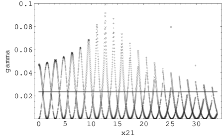
Figure 8: The decay rates $\gamma_{s}$ ($\times$) and $\gamma_{a}$ ($+$) oscillating as a function of $x_{21}$. The solid line is the one-atom decay rate $\gamma_{1}=0.0235$. $\gamma_{s}$ vanishes for distances close to $(2n-1)\pi/{\tilde{\omega}}_{1}$, and $\gamma_{a}$ for distances close to $2n\pi/{\tilde{\omega}}_{1}$ with $n$ integer. An example is $x_{21}=12.7\approx 8\pi/{\tilde{\omega}}_{1}$, where $\gamma_{a}$ vanishes, while $\gamma_{s}$ is large. For large $x_{21}$ the decay rates decrease.

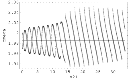
Figure 9: The energies ${\tilde{\omega}}_{s}$ ($\times$) and ${\tilde{\omega}}_{a}$ ($+$) as a function of $x_{21}$. They oscillate with $x_{21}$. The solid line is the one-atom energy ${\tilde{\omega}}_{1}=1.985$.

VI Decay rate and energy vs. distance

Figure 10: Survival probability $P_{1}(t)$ of atom 1 for symmetric (dashed) and antisymmetric (solid) initial conditions and $x_{21}=12.7$. The symmetric state gives rise to a super-radiant, stationary collective state. The antisymmetric state gives rise to a sub-radiant (stationary) collective state. Before $t=x_{21}$, $P_{1}(t)$ has the one-atom decay rate. Time $t$ is in units of $x_{21}$. $P_{1}(t)$ is dimensionless.

Figure 11: Field intensity $P(x,t)$ for the atoms in a stationary collective state. The field between the two atoms, located at $x=0$ and $x=1$ remains trapped. $x$ is in units of $x_{21}=12.7$ and $P(x,t)$ is dimensionless. The initial condition is $|a\rangle$. Time is $t=7.09\,x_{21}$. The wave packets on each side represent the field emitted before the atoms formed the collective state. After this, there is no emission (we have sub-radiance).

Figure 12: Field intensity $P(x,t)$ for initial condition $|s\rangle$ at time $t=7.09\,x_{21}$. $x$ is in units of $x_{21}=12.7$ and $P(x,t)$ is dimensionless. The collective state has decayed. The smaller peaks on the far sides are the field emitted individually by each atom before attaining the collective state. The larger peaks correspond to the two-atom collective emission (super-radiance).

Figure 13: The graph of ${\cal F}_{s}=-d{\tilde{\omega}}_{s}/dx_{21}$ (black line) and the decay rate $-\gamma_{s}$ (dotted line). We see that when $-\gamma_{s}$ is a local minimum ${\cal F}_{s}$ has also a local minimum value.

In this section we investigate the behavior of the complex eigenvalues of the Hamiltonian $z_{j}$ for different values of $x_{21}$.

The equation $\eta^{+}_{j}(z)=0$ can be solved numerically by iterations of $z=z-\eta^{+}_{j}(z)$. The imaginary and real parts of $z$ thus obtained are shown in Figs. 8 and 9 (we used the same parameters as in the previous figures). The numerical iteration was started around $z=\omega_{1}$ so, with the exception of two isolated points seen in Fig. 8, the solutions obtained are the collective eigenvalues $z=z_{j}$. Gaps in the graphs are points missed by the numerical solution.

As we see, $\gamma_{j}$ and ${\tilde{\omega}}_{j}$ oscillate with $x_{21}$. The oscillation period is approximately $2\pi/{\tilde{\omega}}_{1}$ where ${\tilde{\omega}}_{1}$ is the one-atom renormalized frequency (see Appendix B).

Due to the oscillations, the collective decay rate can become smaller or larger than the one-atom decay rate (solid line in Fig. 8). We have sub-radiance and super-radiance, respectively. In particular, it is noticeable that there are distances at which the decay rates $\gamma_{j}$ vanish (see Appendix B). This means that for these distances there is no outgoing radiation. The outgoing emitted fields of the atoms cancel by destructive interference and a standing field is trapped between two atoms, storing energy. Note that both symmetric and antisymmetric initial conditions can give rise to either sub-radiant or super-radiant states, since both $\gamma_{s}$ and $\gamma_{a}$ oscillate with $x_{21}$.

The oscillations of the decay rate and the energy shown in Figs. 8 and 9 are a unique feature of one-dimensional systems. For two or three dimensions, these quantities can change significantly only for short distances between atoms (see Appendix C).

As an example of sub-radiance and super-radiance we show numerical simulations with the same parameters used in the previous examples, except we choose $L=250$ (to have higher space resolution) and $x_{21}=12.7$. For this value of $x_{21}$, the decay rate of the antisymmetric state vanishes while the decay rate of the symmetric state is maximum, (see Fig. 8). In Fig. 10 we show the survival probability of atom 1 for the antisymmetric and symmetric initial conditions, showing the appearance of stationary sub-radiant collective state and a super-radiant collective state. In Figs. 11 and 12 we show the corresponding fields.

We turn to the force between the atoms. Here we will only give a heuristic discussion. A more detailed analysis requires including the Casimir-Polder or van der Waals forces between the atoms, as well as the inertia of the atoms, which we are not considering in this paper.

Since the atoms are unstable, the force between them should be time-dependent Passante . We expect the force will decay exponentially during the time scales where the collective-state components dominate. For the dependence on $x_{21}$ of the force, the quantity

$${\cal F}_{j}=-d{\tilde{\omega}}_{j}/dx_{21}$$ (86)

can give an indication because ${\tilde{\omega}}_{j}$ is the average energy of the collective state.

As we can see in Figure 13, ${\cal F}_{s}$ oscillates with $x_{21}$ (${\cal F}_{a}$ has a similar behavior). ${\cal F}_{s}>0$ corresponds to a repulsive force, and ${\cal F}_{s}<0$ to an attractive force. The attractive force between two atoms becomes locally maximum when the collective decay rate is locally maximum. The atoms tend to attract each other when they emit the field outwards, and tend to repel when the field remains trapped between them.

Also we see in Fig. 13 that there are points $x_{21}^{0}$ for which ${\cal F}_{s}$ vanishes. If $d{\cal F}_{s}/dx_{21}<0$ at these points, then any small displacement $\Delta x_{21}$ around $x_{21}^{0}$ creates a force in the opposite direction. Thus in this case $x_{21}^{0}$are stable points [if $d{\cal F}_{s}/dx_{21}>0$ the points are unstable]. The existence of stable points suggests the possibility of having a one-dimensional “molecule.” This molecule would have a lifetime of the order of $\gamma_{s}^{-1}$.

VII Two-cavity wave guides

Figure 14: A two-cavity waveguide

As shown in Refs. Suresh0 ; Suresh , a Hamiltonian of the form (21) can be used to describe a two-dimensional electron wave guide as seen in Fig. 14.

This wave guide can be constructed by superposing two closed identical cavities and a lead. This forms the unperturbed system. The interaction appears as the cavities and the lead are connected.

In suitable units the horizontal dimension of the cavities is $1$, and the vertical dimension is $D$. The lead has a horizontal dimension $L\to\infty$ and a vertical dimension $W$. We consider a non-relativistic electron, neglecting the spin.

If the electron is placed inside a closed cavity, its wave functions correspond to discrete cavity modes. The cavity modes can be labeled as $|m,n\rangle$, where $m$, $n$ are positive integers representing the horizontal and vertical wave numbers. The corresponding energies are

$$\xi^{m,n}=m^{2}+n^{2}/D^{2}$$ (87)

An electron placed inside the lead (with no cavities) has modes that can be labeled as $|k,l\rangle$ where $kL/\pi$ is the horizontal wave number and $l$ the vertical wave number. The energies are

$$E_{k,l}=k^{2}/\pi^{2}+l^{2}/W^{2}$$ (88)

As $L\to\infty$, $k$ becomes a continuous variable. On the other hand, $m$, $n$ and $l$ are always integers.

We consider an electron with low energy narrowly centered around

$$\xi^{0}=\xi^{m_{0},n_{0}}$$ (89)

We assume that

$$E_{0,1}<\xi^{0}<E_{k,l}$$ (90)

for $l>1$ and all $k$. The electron may propagate through the first mode of the lead, but not through the $l>1$ modes.

We also assume that there are no other cavity modes with energy between $E_{0,1}$ and $\xi_{0}$. Under these conditions, the cavity mode $\xi^{0}$ behaves essentially like the excited state in the Friedrichs-Lee model. It will decay with a finite lifetime. This means than an electron inside the cavity will escape through the lead.

The following approximate Hamiltonian is obtained Suresh .

$$H_{WG} = \xi^{0}[|1\rangle\langle 1|+|2\rangle\langle 2|]+\sum_{k,l}E_{k,l}|\psi_{k,l}\rangle\langle\psi_{k,l}|$$

$$+ \sum_{k,l}V^{0}_{k,l}\left(|1\rangle\langle\psi_{k,l}|e^{ikx_{1}}+|2\rangle\langle\psi_{k,l}|e^{ikx_{2}}\right)+\rm{h.c.}$$

Here, h.c. means Hermitian conjugate. The cavities are centered at $x=x_{1}$ and $x=x_{2}$, where $x$ is the horizontal coordinate. The states $|i\rangle$ represent the electron inside cavity $i=1$ or $2$, occupying the mode $\xi_{0}$. The states $|\psi_{k,l}\rangle$ are modified lead modes; they essentially represent the electron inside the part of the lead that does not overlap with the cavities. The terms $V^{0}_{k,l}$ represent the amplitude of a transition of the electron from this part of the lead to the cavities or vice versa. Their detailed expression is given in Ref. Suresh .

Except for the additional index $l$ and the dispersion relation (88), which is different from $\omega_{k}=|k|$, the Hamiltonian $H_{WG}$ is the same as our two-atom Hamiltonian (21). As the two cavities are identical, we have a system analogous to the two identical atoms. Since there is only one continuous variable $k$ describing the propagation along the lead, we can think of the wave guide system as a one-dimensional system, with internal degree of freedom $l$ (note that $l$ is discrete).

Using the results of the Sec. III we obtain the equation for the complex energy of the collective state

$$z^{0}_{j}=\xi^{0}+2\int_{0}^{\infty}dk\sum_{l=1}^{\infty}\frac{|v^{0}_{k,l}|^{2}}{(z^{0}_{j}-E_{k,l})^{+}}(1+\sigma_{j}\cos kx_{21})$$

(92)

where $v^{0}_{k,l}=(L/\pi)V^{0}_{k,l}$. We will show that there is a solution with vanishing decay rate, corresponding to a stable collective state. We follow the procedure shown in Appendix B. For a vanishing decay rate we write $z^{0}_{j}={\tilde{\xi}}^{0}_{j}-i\epsilon$, where $\epsilon>0$ is infinitesimal. This gives the following condition on $x_{21}$:

$$1+\sigma_{j}\cos k_{0}x_{21}=0$$ (93)

where $k_{0}$ is a wave vector that satisfies

$$E_{k_{0},l}={\tilde{\xi}}^{0}_{j},\quad l=1$$ (94)

Through these two equations, $x_{21}$ becomes a function of ${\tilde{\xi}}^{0}_{j}$,

$$x_{21}=g({\tilde{\xi}}^{0}_{j})\equiv\frac{n}{\sqrt{{\tilde{\xi}}^{0}_{j}-E_{0,1}}}$$ (95)

where $n=$ odd integer for $j=s$, and $n=$ even integer for $j=a$. The renormalized energy ${\tilde{\xi}}^{0}_{j}$ is then given by the solution of the integral equation

$${\tilde{\xi}}_{j}^{0} = \xi_{0}$$

$$+ 2\int_{0}^{\infty}dk\sum_{l=1}^{\infty}|v_{k,l}^{0}|^{2}\frac{{\cal P}}{{\tilde{\xi}}_{j}^{0}-E_{k,l}}\left[1+\sigma_{j}\cos[kg({\tilde{\xi}}^{0}_{j})]\right]$$

where ${\cal P}$ means principal part. Similar to Eq. (LABEL:G8), this equation has a solution if the condition

$$\xi^{0}-E_{0,1}>2\int_{0}^{\infty}dk\sum_{l=1}^{\infty}|v_{k,l}^{0}|^{2}\frac{{\cal P}}{E_{k,l}-E_{0,1}}$$ (97)

is satisfied. If the two cavities are not too close, we can replace the interaction $v_{k,l}^{0}$ by the interaction in a single-cavity system. Then, Eq. (97) is essentially the condition that the electron in an individual cavity has enough energy $\xi^{0}$ to escape through the lead. This condition is analogous to Eq. (6).

In summary, adjusting the distance between the cavities, so that Eq. (95) is satisfied, we obtain a collective stable state where the electron remains trapped inside the two cavities, in either a symmetric or antisymmetric state. The electron is trapped even though it would escape if there was only one cavity.

To obtain this result we neglected the influence of cavity modes other than $\xi^{0}$. The existence of stable configurations in the wave guide could be verified by other methods, including numerical simulations or experiments.

VIII Concluding remarks

We have analyzed a two-atom system using complex collective eigenstates of the Hamiltonian. Our main result is the description of long-range effects in one-dimensional space, such as the vanishing of the decay rate at regular intervals of distance $x_{21}$. Another result is the application of this model to two-dimensional electron wave guides, where a two-cavity configuration can be tuned to act as an electron trap.

In our two-atom model we neglected virtual transitions. This corresponds to a rotating wave approximation. Phenomena such as the existence of collective stable states in one-dimensional atoms deserve further study, with the inclusion of virtual transitions. Electron wave guides, on the other hand, are already well described by the type of Hamiltonian we considered, without virtual transitions. The description improves if we include more cavity modes Suresh .

Emitted photons are described by an exponentially growing field, truncated at the light cone of the atoms. This field plays an important role in the two-atom system, giving a strong influence on the lifetime or average energy of the collective states. This field is directly related to the exponential decay of unstable states, which can be regarded as one of the simplest dissipative phenomena on a microscopic scale. So, in a sense, the formation of collective states is a microscopic non-equilibrium process, driven by dissipation.

Appendix A Proof of Eq. (81)

We start with the expression (see Eq. (80))

$${{\tilde{I}}}_{0}(t)=\frac{1}{2\pi i}\sum_{n=0}^{\infty}\int_{C}dk\,\frac{\Delta(k)^{n}}{(k-z_{s1})^{n+1}}e^{-ikt}$$ (98)

where $C$ is a clockwise contour surrounding $k=z_{s1}$. Taking the residues at this point we get

$${{\tilde{I}}}_{0}(t)=\sum_{n=0}^{\infty}\frac{-1}{n!}\frac{\partial^{n}}{\partial k^{n}}[\Delta(k)^{n}e^{-ikt}]_{k=z_{s1}}$$ (99)

This is a perturbation expansion around $z_{s1}$, so it will correspond only the contribution from the pole $z_{s}$ and not the poles $z_{s,n}$.

We will show that

$$\frac{\partial}{\partial t}{{\tilde{I}}}_{0}(t)=-iz_{s}{{\tilde{I}}}_{0}(t).$$ (100)

Together with Eq. (85) this will prove Eq. (81). Starting with Eq. (99) and using

$$\frac{\partial^{n}}{\partial k^{n}}AB=\sum_{l=0}^{n}\frac{n!}{l!(n-l)!}\left[\frac{\partial^{n-l}}{\partial k^{n-l}}A\right]\left[\frac{\partial^{l}}{\partial k^{l}}B\right]$$ (101)

we obtain

$$\frac{\partial}{\partial t}{{\tilde{I}}}_{0}(t)=-iz_{s1}{{\tilde{I}}}_{0}(t)-i{\tilde{I}}_{1}(t)$$ (102)

where

$${{\tilde{I}}}_{m}(t)=\sum_{n=0}^{\infty}\frac{-1}{n!}\frac{\partial^{n}}{\partial k^{n}}[\Delta(k)^{n+m}e^{-ikt}]_{k=z_{s1}}$$ (103)

Using Eq. (101) again we get

$${{\tilde{I}}}_{m}(t)=\sum_{l=0}^{\infty}\frac{1}{l!}{\tilde{I}}_{l}(t)\frac{\partial^{l}}{\partial k^{l}}[\Delta(k)^{m}]_{k=z_{s1}}$$ (104)

With Eq. (84) for $z_{s,0}=z_{s}$ and the Taylor expansion of $\Delta(z_{s})^{l}$ around $z_{s1}$ we find that the solution of this system of equations is

$${{\tilde{I}}}_{l}(t)=\Delta(z_{s})^{l}{\tilde{I}}_{0}(t)$$ (105)

which combined with Eq. (102) proves Eq. (100).

Appendix B Oscillations of $\gamma_{j}$ and $\omega_{j}$ with $x_{21}$

In this Appendix we will show that the decay rates $\gamma_{j}$ and energies ${\tilde{\omega}}_{j}$ of the collective states $|\phi_{j}\rangle$ oscillate with the distance $x_{21}$ between the atoms. First we will show that $\gamma_{s}$ vanishes (comes infinitesimally close to zero) for distances

$$[x_{21}]_{\gamma_{s}=0}=\frac{(2n+1)\pi}{{\tilde{\omega}}_{s}^{o}}$$ (106)

where $n$ is an integer, and

$${\tilde{\omega}}_{s}^{o}=[{\tilde{\omega}}_{s}]_{\gamma_{s}=0}$$ (107)

Similarly we will show that decay rate $\gamma_{a}$ vanishes for

$$[x_{21}]_{\gamma_{a}=0}=\frac{2n\pi}{{\tilde{\omega}}_{a}^{o}}$$ (108)

where

$${\tilde{\omega}}_{a}^{o}=[{\tilde{\omega}}_{a}]_{\gamma_{a}=0}.$$ (109)

We start with the equation $\eta^{+}_{s}(z_{s})=0$ or

$$z_{s}=\omega_{1}+2\int_{0}^{\infty}dk\frac{\lambda^{2}v_{k}^{2}}{(z_{s}-k)^{+}}(1+\cos kx_{21})$$ (110)

Assuming $z_{s}={\tilde{\omega}}_{s}^{o}-i\epsilon$ with infinitesimal $\epsilon$ we have

$${\tilde{\omega}}_{s}^{o} = \omega_{1}+2\int_{0}^{\infty}dk\frac{\lambda^{2}v_{k}^{2}}{{\tilde{\omega}}_{s}^{o}-k+i\epsilon}(1+\cos kx_{21})$$ (111)

$$= \omega_{1}+2\int_{0}^{\infty}dk\lambda^{2}v_{k}^{2}\left[\frac{{\cal P}}{{\tilde{\omega}}_{s}^{o}-k}-\pi i\delta({\tilde{\omega}}_{s}^{o}-k)\right]$$

$$\times (1+\cos kx_{21})$$

where we used the relation

$$\frac{1}{\omega+i\epsilon}=\frac{{\cal P}}{\omega}-\pi i\delta(\omega)$$ (112)

together with Eq. (14). Comparing the left and right-hand sides of Eq. (111) we see that the imaginary part should vanish, so we get

$$1+\cos{\tilde{\omega}}_{s}^{o}x_{21}=0$$ (113)

which proves Eq. (106). In a similar way, starting from the equation for $z_{a}$,

$$z_{a}=\omega_{1}+2\int_{0}^{\infty}dk\frac{\lambda^{2}v_{k}^{2}}{(z_{a}-k)^{+}}(1-\cos kx_{21})$$ (114)

we get

$$1-\cos{\tilde{\omega}}_{a}^{o}x_{21}=0$$ (115)

which proves Eq. (108).

The ${\tilde{\omega}}_{j}^{o}$ satisfy the integral equations

$${\tilde{\omega}}_{s}^{o} = \omega_{1}+2\int_{0}^{\infty}dk\lambda^{2}v_{k}^{2}\frac{{\cal P}}{{\tilde{\omega}}_{s}^{o}-k}\left[1+\cos\frac{(2n+1)\pi k}{{\tilde{\omega}}_{s}^{o}}\right]$$

$${\tilde{\omega}}_{a}^{o} = \omega_{1}+2\int_{0}^{\infty}dk\lambda^{2}v_{k}^{2}\frac{{\cal P}}{{\tilde{\omega}}_{a}^{o}-k}\left[1-\cos\frac{2n\pi k}{{\tilde{\omega}}_{a}^{o}}\right]$$

Using graphical methods it can be shown the first equation has a unique solution for each integer $n$, provided that

$$\omega_{1}-2\lim_{{\tilde{\omega}}_{s}^{o}\to 0}\int_{0}^{\infty}dk\lambda^{2}v_{k}^{2}\frac{{\cal P}}{k}\left[1+\cos\frac{(2n+1)\pi k}{{\tilde{\omega}}_{s}^{o}}\right]>0$$

(117)

In the limit ${\tilde{\omega}}_{s}^{o}\to 0$ the cosine term gives a vanishing integration. Thus Eq. (117) is satisfied if Eq. (6) is satisfied. A similar argument applies to the second equation in (LABEL:G8).

Eqs. (106) and (108) explain the oscillatory behavior of $\gamma_{j}$ seen in Fig. 8.

To explain the oscillations of ${\tilde{\omega}}_{j}$ we note that the terms inside brackets in Eq. (LABEL:G8) are even in $k$ around ${\tilde{\omega}}_{j}^{o}$, regardless of $n$. On the other hand, the principal parts are odd. Hence the product is odd and the integration around ${\tilde{\omega}}_{j}^{o}$ vanishes. Thus the largest contributions to the integrals come from the tails of the principal parts. The “$1$” terms inside the brackets give a much larger contribution than the “$\cos$” terms, because the latter oscillate with $k$. Neglecting the “$\cos$” terms we get

$${\tilde{\omega}}_{s}^{o}\approx{\tilde{\omega}}_{a}^{o}\approx{\tilde{\omega}}_{1}$$ (118)

where ${\tilde{\omega}}_{1}$ is the one-atom shifted energy (see Eq. (16)). This shows that the ${\tilde{\omega}}_{j}$ have approximately the same values when their respective $\gamma_{j}$ vanish. From Eq. (118) we conclude that the period of the oscillations of $\gamma_{j}$ and ${\tilde{\omega}}_{j}$ is approximately $2\pi/{\tilde{\omega}}_{1}$.

Adding Eqs. (110) and (114) we see that for weak coupling the poles of the one and two-atom Green functions obey the relations

$$z_{1}\approx\frac{z_{a}+z_{s}}{2}$$ (119)

So both ${\tilde{\omega}}_{j}$ and $\gamma_{j}$ oscillate around the one-atom ${\tilde{\omega}}_{1}$ and $\gamma_{1}$, respectively.

Finally, we show that the “force” ${\cal F}_{s}$ between the atoms is a maximum when the decay rate is zero, as seen in Fig. 13. When $\gamma_{s}=0$, we have

$$\frac{d{\cal F}_{s}^{o}}{dx_{21}}=-\frac{d^{2}{\tilde{\omega}}_{s}^{o}}{dx_{21}^{2}}$$ (120)

$$\approx 2\int_{0}^{\infty}dk\lambda^{2}v_{k}^{2}\frac{{\cal P}}{{\tilde{\omega}}_{s}^{o}-k}k^{2}\cos\frac{(2n+1)\pi k}{{\tilde{\omega}}_{s}^{o}}$$

As argued above Eq. (118) the integral of the cosine is small. Hence we have

$$\frac{d{\cal F}_{s}^{o}}{dx_{21}}\approx 0$$ (121)

A similar argument may be applied to ${\cal F}_{a}$.

Appendix C Sub-radiance in $d>1$ dimensions

In one dimension, the vanishing of the collective decay rate occurs for distances given by the conditions

$$1+\sigma_{j}\cos{\tilde{\omega}}_{j}^{o}x_{21}=0$$ (122)

Assuming the potential $v_{k}$ is rotationally invariant, in $d>1$ dimensions, analogous conditions would be

$$\int_{0}^{\pi}\Omega(\theta)d\theta[1+\sigma_{j}\cos({\tilde{\omega}}_{j}^{o}x_{21}\cos\theta)]=0$$ (123)

where $\theta$ is the angle of the wave vector ${\bf k}$, with respect to the line joining the two atoms. The function $\Omega$ is $2$ for $d=1$ and $\sin\theta$ for $d=3$.

We see that Eq. (123) can only be satisfied for the antisymmetric state with $\sigma_{j}=-1$ and for short distances $x_{21}\ll{\tilde{\omega}}_{j}^{o}\approx{\tilde{\omega}}_{1}^{-1}$. This agrees with the results of Stephen Stephen anticipated by Dicke Dicke .

References

(1) R. H. Dicke, Phys. Rev. 93, 99 (1954).
(2) W. Woger, H. King, R. Glauber, and J. H. Haus, Phys. Rev. A 34, 4859 (1986).
(3) C. Compgano, G. M. Palma, R. Passante and F. Persico, J. Phys. B
28, 1105 (1995).
(4) M. J. Stephen, J. Chem. Phys. 50, 669 (1964).
(5) P.W. Milonni and P. L. Knight, Phys. Rev. A 10, 1096 (1974).
(6) H. T. Dung and K. Ujihara, Phys. Rev. A 59, 2524 (1999).
(7) E.A. Power and T. Thirunamachandran, Phys. Rev. A 51, 3660 (1995); Phys. Rev. A 47, 2539 (1993).
(8) H. T. Dung and K. Ujihara, Phys. Rev. Lett. 84, 254 (2000).
(9) G.I. Kweon and N. M. Lawandy, Phys. Rev. A 47, 4513 (1993);
Phys. Rev. A 49, 2205 (1994).
(10) Z. Ficek, Phys. Rev. A 44, 7759 (1991).
(11) N. Nakanishi, Prog. Theor. Phys. 19, 607 (1958).
(12) E.C.G. Sudarshan, C. B. Chiu and V. Gorini, Phys. Rev. D
18, 2914 (1978).
(13) A. Böhm and M. Gadella, Dirac Kets, Gamow Vectors and Gelfand
Triplets, (Springer Lecture Notes on Physics, Vol. 348, Springer, New
York, 1989).
(14) T. Petrosky, I. Prigogine and S. Tasaki, Physica A 173, 175
(1991).
(15) T. Petrosky, G. Ordonez and I. Prigogine,
Phys. Rev. A 64, 062101 (2001).
(16) S. Kim and G. Ordonez, arXiv:physics/0311048 (2003).
(17) T. Petrosky and S. Subbiah, Physica E 19, 230 (2003);
(18) S. Subbiah, Dissertation, The University of Texas at Austin (2000).
(19) U. Weiss, Quantum Dissipative Systems (World Scientific, Singapore, 1993).
(20)
P. Facchi and S. Pascazio, Physica A 271, 133 (1999).
(21) T. Petrosky, G. Ordonez and I. Prigogine,
Phys. Rev. A 62, 042106 (2000).
(22) C. Cohen-Tannouji, J. Dupont-Roc and G. Grynberg, Atom-photon
interactions. Basic processes and applications (Wiley, New York,
1992), p. 248.
(23) http://www.netlib.org/eispack/
(24) R. Passante and F. Persico,
arXiv:quant-ph/0212163 (2002).