Abstract

It has been almost one hundred years since Einstein formulated his special theory of relativity in 1905. He showed that the basic space-time symmetry is dictated by the Lorentz group. It is shown that this group of Lorentz transformations is not only applicable to special relativity, but also constitutes the scientific language for optical sciences. It is noted that coherent and squeezed states of light are representations of the Lorentz group. The Lorentz group is also the basic underlying language for classical ray optics, including polarization optics, interferometers, the Poincareé sphere, one-lens optics, multi-lens optics, laser cavities, as well multilayer optics.

1 Introduction

Since Einstein formulated special relativity in 1905, the basic space-time symmetry has been that of the Lorentz group. He established the energy-momentum relation which is valid for slow massive particles, high-speed massive particles, and massless particles. Einstein formulated this relation initially for particles without internal space-time structures, but it is widely accepted that it is valid for all particles including particles with spin and/or internal space-time extension.

In 1939, Wigner published his most fundamental paper dealing with internal space-time symmetries of relativistic particles [1]. In this paper, Wigner introduced the Lorentz group to physics. Furthermore, by introducing his “little groups,” Wigner provided the framework for studying the internal space-time symmetries of relativistic particles. The scientific contents of this paper have not yet been fully recognized by the physics community. We are writing this report as a continuation of the work Wigner initiated in this history-making paper.

While particle physicists are still struggling to understand internal space-time symmetries of elementary particles, Wigner’s Lorentz group is becoming useful to many other branches of physics. Among them are optical sciences, both quantum and classical. In quantum optics, the coherent and squeezed states are representations of the Lorentz group [2]. Recently, the Lorentz group is becoming the fundamental language for classical ray optics. It is gratifying to note that optical components, such as lenses, polarizers, interferometers, lasers, and multi-layers can all be formulated in terms of the Lorentz group which Wigner formulated in his 1939 paper. Classical ray optics is of course a very old subject, but we cannot do new physics without measurements using optical instruments. Indeed, classical ray optics constitutes Wigner’s frontier in physics.

The word ”group theory” sounds like abstract mathematics, but it is gratifying to note that Wigner’s little groups can be formulated in terms of two-by-two matrices, while classical ray optics is largely a physics of two-by-two matrices. The mathematical correspondence is straight-forward.

In order to see this point clearly, let us start with the following classic example. The second-order differential equation

$$A{d^{2}q(t)\over dt^{2}}+B{dq(t)\over dt}+Cq(t)=F\cos(\omega t).$$ (1)

is applicable to a driven harmonic oscillator with dissipation. This can also be used for studying an electronic circuits consisting of inductance, resistance, capacitance, and an alternator. Thus, it is possible to study the oscillator system using an electronic circuit. Likewise, an algebra of two-by-two matrices can serve as the scientific language for several different branches of physics, including special relativity, ray optics, and quantum optics.

Table 1: Further contents of Einstein’s $E=mc^{2}$. Massive and massless particles have different energy-momentum relations. Einstein’s special relativity gives one relation for both. Wigner’s little group unifies the internal space-time symmetries for massive and massless particles. The quark model and the parton model can also be combined into one covariant model.

	Massive, Slow	COVARIANCE	Massless, Fast
Energy-		Einstein’s
Momentum	$E=p^{2}/2m_{0}$	$E=\sqrt{p^{2}c^{2}+m_{0}^{2}c^{4}}$	$E=cp$
Internal	$S_{3}$		$S_{3}$
space-time		Wigner’s
symmetry	$S_{1},S_{2}$	Little Group	Gauge Trans.
Relativistic		Lorentz-squeezed
Extended	Quarks	Harmonic	Partons
Particles		Oscillators

There are many physical systems which can be formulated in terms of two-by-two matrices. If we restrict that their determinant be one, there is a well established mathematical discipline called the group theory of $SL(2,C)$. This aspect was noted in the study of Lorentz transformations. In group theoretical terminology, the group $SL(2,C)$ is the universal covering group of the group of the Lorentz group. In practical terms, to each two-by-two matrix, there corresponds one four-by-four matrix which performs a Lorentz transformation in the four-dimensional Minkowskian space. Thus, if a physical system can be explained in terms of two-by-two matrices, it can be explained with the language of Lorentz transformations. Furthermore, the physical system based on two-by-two matrices can serve as an analogue computer for Lorentz transformations.

Optical filters, polarizers, and interferometers deal with two independent optical rays. They superpose the beams, change the relative phase shift, and change relative amplitudes. The basic language here is called the Jones matrix formalism, consisting of the two-by-two matrix representation of the $SL(2,C)$ group [3, 4]. The four-by-four Mueller matrices are derivable from the two-by-two matrices of $SL(2,C)$.

For these two-beam systems, the Poincaré sphere serves as an effective language [5, 6]. Since the two-beam system is described by the Lorentz group, the Poincaré sphere is necessarily a representation of the Lorentz group. We shall use this sphere to study the degree of coherence between the beams.

Para-axial lens optics can also be formulated in terms of two-by-two matrices, applicable to the two-component vector space consisting of the distance from the optical axis and the slope with respect to the axis. The lens and translation matrices are triangular, but they are basically representations of the $Sp(2)$ group which is the real subgroup of the group $SL(2,C)$ [7, 8].

Laser optics is basically multi-lens lens optics. However, the problem here is how to get a simple mathematical expression for the system of a large number of the same lens separateled by equal distance. Here again, group theory simplifies calculations [9].

In multi-layer optics, we deal with two optical rays moving in opposite directions. The standard language in this case is the S-matrix formalism [10]. This is also a two-by-two matrix formalism. As in the case of laser cavities, the problem is the multiplication of a large number of matrix chains [11, 12].

It is shown in this report that the two-by-two representation of the six-parameter Lorentz group is the underlying common scientific language for all of the instruments mentioned above. While the abstract group theoretical ideas make two-by-two matrix calculations more systematic and transparent in optics, optical instruments can act as analogue computers for Lorentz transformations in special relativity. It is gratifying to note that special relativity and ray optics can be formulated as the physics of two-by-two matrices.

In Sec. 2, we explain how the Lorentz group can be formulated in terms of four-by-four matrices. It is shown that the group can have six independent parameters. In Sec. 3, we explain how it is possible to formulate the Lorentz group in terms of two-by-two matrices. It is shown that the four-by-four transformation matrices can be constructed from those those of the two-by-two matrices.

In Sec. 4, we discuss the historical significance of Wigner’s 1939 paper [1] on the Lorentz group and its application to the internal space-time symmetries of relativistic particles. In Sec. 5, we present the basic building blocks for the two-by-two representation of the Lorentz group in terms of the matrices commonly seen in ray optics.

In Secs. 5 and 6, we study the polarizations for the two-beam system. It is shown that both the Jones and Mueller matrices are representations of the Lorentz group. The role of the Stokes parameters is discussed in detail. It is shown in Sec. 9 that the Poincaré sphere is a graphical representation of the Poincaré group, and serves as a device to describe the degree of coherence.

In Secs. 10, 11, 12, and 13, we discuss one-lens system, multi-lens system, laser cavities, and multi-layer optics, respectively. In all of these sections, the central scientific language is the Lorentz group.

In Appendix A, we expand the content of the third row of Table 1. It is noted that the covariant harmonic oscillator formalism can unify the quark model for slow hadrons with the parton model for ultra-relativistic quarks. It is then shown that the same oscillator formalism serves as the basic scientific language for squeezed states of light.

In Appendix B, it is shown that the Lie-group method, in terms of the generators, is not the only method in constructing group representations. For the rotation group and the three-parameter subgroups of the Lorentz group, it is simpler to start with the minimum number of starter matrices. For instance, while there are three generators for the rotation group in the Lie approach, we can construct the most general form of the rotation matrix from rotations around two directions, as Goldstein constructed the Euler angles [13].

In Appendix C, it is noted that the four-by-four matrices are real, their two-by-two counterparts are complex. However, there is a three-parameter real subgroup called $Sp(2)$. It is shown that the complex subgroup $SU(1,1)$ is equivalent to $Sp(2)$ through conjugate transformation.

2 Lorentz Transformations

Let us consider the space-time coordinates $(ct,z,x,y)$. Then the rotation around the $z$ axis is performed by the four-by-four matrix

$$\pmatrix{1&0&0&0\cr 0&0&0&0\cr 0&0&\cos\theta&-\sin\theta\cr 0&0&\sin\theta&\cos\theta}.$$ (2)

This transformation is generated by

$$J_{3}=\pmatrix{0&0&0&0\cr 0&0&0&0\cr 0&0&0&-i\cr 0&0&i&0}.$$ (3)

Likewise, we can write down the generators of rotations $J_{1}$ and $J_{2}$ around the $x$ and $y$ axes respectively.

$$J_{1}=\pmatrix{0&0&0&0\cr 0&0&0&i\cr 0&0&0&0\cr 0&-i&0&0},\qquad J_{2}=\pmatrix{0&0&0&0\cr 0&0&-i&0\cr 0&i&0&0\cr 0&0&0&0}.$$ (4)

These three generators satisfy the closed set of commutations relations

$$\left[J_{i},J_{j}\right]=i\epsilon_{ijk}J_{k}.$$ (5)

This set of commutation relations is for the three-dimensional rotation group.

The Lorentz boost along the $z$ axis takes the form

$$B=\pmatrix{\cosh\eta&\sinh\eta&0&0\cr\sinh\eta&\cosh\eta&0&0\cr 0&0&1&0\cr 0&0&0&1},$$ (6)

which is generated by

$$K_{3}=\pmatrix{0&i&0&0\cr i&0&0&0\cr 0&0&0&0\cr 0&0&0&0}.$$ (7)

Likewise, we can write generators of boosts $K_{1}$ and $K_{2}$ along the $x$ and $y$ axes respectively, and they take the form

$$K_{1}=\pmatrix{0&0&i&0\cr 0&0&0&0\cr i&0&0&0\cr 0&0&0&0},\qquad K_{2}=\pmatrix{0&0&0&i\cr 0&0&0&0\cr 0&0&0&0\cr i&0&0&0}.$$ (8)

These boost generators satisfy the commutation relations

$$\left[J_{i},K_{j}\right]=i\epsilon_{ijk}K_{k},\qquad\left[K_{i},K_{j}\right]=-i\epsilon_{ijk}J_{k}.$$ (9)

Indeed, the three rotation generators and the three boost generators satisfy the closed set of commutation relations given in Eq.(5) and Eq.(9). These three commutation relations form the starting point of the Lorentz group. The generators given in this section are four-by-four matrices, but they are not the only set satisfying the commutation relations. We can construct also six two-by-two matrices satisfying the same set of commutation relations. The group of transformations constructed from these two-by-two matrices is often called $SL(2,c)$ or the two-dimensional representation of the Lorentz group. Throughout the present paper, we used the two-by-two transformation matrices constructed from the generators of the $SL(2,c)$ group.

3 Spinors and Four-vectors

In Sec. 2, we started with four-by-four transformation matrices applicable to the four-dimensional space-time. We then ended up with a set of closed commutation relations for the six generators consisting of three rotation and three boost generators. These generators are in the form of four-by-four matrices.

In this section, we shall see first that there is a set of two-by-two matrices satisfying the same set of commutation relations, constituting the two-by-two representations of the Lorentz group. The representation so constructed is called the $SL(2,c)$ group, or the universal covering group of the Lorentz group. The transformation matrices are applicable to two-component $SL(2,C)$ spinors. The algebraic property of this two-by-two representation is the same as that of the four-by-four representation.

As we shall see in this paper, the spinors and the four-vectors correspond to Jones vectors and Stokes parameters respectively in polarization optics [4]. The question then is whether we can construct the four-vector from the spinors. In the language of polarization optics, the question is whether it is possible to construct the coherency matrix [5, 6] from the Jones vector.

With this point in mind, let us start from the following form of the Pauli spin matrices:

$$\sigma_{1}=\pmatrix{1&0\cr 0&-1},\quad\sigma_{2}=\pmatrix{0&1\cr 1&0},\quad\sigma_{3}=\pmatrix{0&-i\cr i&0}.$$ (10)

These matrices are written in a different convention. Here $\sigma_{3}$ is imaginary, while $\sigma_{2}$ is imaginary in the traditional notation. Also in this convention, we can construct three rotation generators

$$J_{i}={1\over 2}\sigma_{i},$$ (11)

which satisfy the closed set of commutation relations

$$\left[J_{i},J_{j}\right]=i\epsilon_{ijk}J_{k}.$$ (12)

We can also construct three boost generators

$$K_{i}={i\over 2}\sigma_{i},$$ (13)

which satisfy the commutation relations

$$\left[K_{i},K_{j}\right]=-i\epsilon_{ijk}J_{k}.$$ (14)

The $K_{i}$ matrices alone do not form a closed set of commutation relations, and the rotation generators $J_{i}$ are needed to form a closed set:

$$\left[J_{i},K_{j}\right]=i\epsilon_{ijk}K_{k}.$$ (15)

The six matrices $J_{i}$ and $K_{i}$ form a closed set of commutation relations, and they are like the generators of the Lorentz group applicable to the (3 + 1)-dimensional Minkowski space. The group generated by the above six matrices is called $SL(2,c)$ consisting of all two-by-two complex matrices with unit determinant.

Let us write the two-by-two transformation matrix as

$$L=\pmatrix{\alpha&\beta\cr\gamma&\delta}.$$ (16)

This matrix has four complex elements with eight real parameters. However, the six generators are all traceless and, the determinant of the matrix has to be one. Thus, it has six independent parameters.

In order to construct four-vectors, we need two different spinor representations of the Lorentz group. Let us go to the commutation relations for the generators given in Eqs.(12), (14) and (15). These commutators are not invariant under the sign change of the rotation generators $J_{i}$, but are invariant under the sign change of the squeeze operators $K_{i}$. Thus, to each spinor representation, there is another representation with the squeeze generators with opposite sign. This allows us to construct another representation with the generators:

$$\dot{J}_{i}={1\over 2}\sigma_{i},\qquad\dot{K}_{i}={-i\over 2}\sigma_{i}.$$ (17)

We call this representation the “dotted” representation. If we write the transformation matrix $L$ of Eq.(16) in terms of the generators as

$$L=\exp\left\{-{i\over 2}\sum_{i=1}^{3}\left(\theta_{i}\sigma_{i}+i\eta_{i}\sigma_{i}\right)\right\},$$ (18)

then the transformation matrix in the dotted representation becomes

$$\dot{L}=\exp\left\{-{i\over 2}\sum_{i=1}^{3}\left(\theta_{i}\sigma_{i}-i\eta_{i}\sigma_{i}\right)\right\}.$$ (19)

In both of the above matrices, Hermitian conjugation changes the direction of rotation. However, it does not change the direction of boosts. We can achieve this only by changing $L$ to $\dot{L}$, and we shall call this the “dot” conjugation.

Likewise, there are two different set of spinors. Let us use write

$$\pmatrix{u\cr v},\quad\pmatrix{\dot{u}\cr\dot{v}}$$ (20)

for the spinor in the undotted and dotted representations respectively. Then the four-vectors are constructed as [14, 15]

$$u\dot{u}=-(x-iy),\quad v\dot{v}=(x+iy),$$

$$u\dot{v}=(t+z),\quad v\dot{u}=-(t-z)$$ (21)

leading to the matrix

$$V=\pmatrix{u\dot{v}&-u\dot{u}\cr v\dot{v}&-v\dot{u}}=\pmatrix{u\cr v}\pmatrix{\dot{v}&-\dot{u}},$$ (22)

where $u$ and $\dot{u}$ are one if the spin is up, and are zero if the spin is down, while $v$ and $\dot{v}$ are zero and one for the spin-up and spin-down cases.

If the two-by-two matrix of Eq. 16 is applicable to the column vector of Eq.(20), what is the transformation matrix applicable to the row vector $(\dot{v},~{}-\dot{u})$ from the right-hand side? It is the transpose of the matrix applicable to the column vector $(\dot{v},~{}-\dot{u})$. We can obtain this column vector from

$$\pmatrix{\dot{v}\cr-\dot{u}},$$ (23)

by applying to it the matrix

$$g=-i\sigma_{3}=\pmatrix{0&-1\cr 1&0}.$$ (24)

This matrix also has the property

$$g\sigma_{i}g^{-1}=-\left(\sigma_{i}\right)^{T},$$ (25)

where the superscript $T$ means the transpose of the matrix. The transformation matrix applicable to the column vector of Eq.(23) is $\dot{L}$ of Eq.(19). Thus the matrix applicable to the row vector $(\dot{v},~{}-\dot{u})$ in Eq.(22) is

$$\left\{g^{-1}Lg\right\}^{T}=g^{-1}L^{T}g.$$ (26)

This is precisely the Hermitian conjugate of $L$.

Let us now write the $V$ matrix of Eq.(22) as

$$V=\pmatrix{t+z&x-iy\cr x+iy&t-z},$$ (27)

where the set of variables $(x,y,z,t)$ is transformed like a four-vector under Lorentz transformations. Then the Lorentz transformation on $V$ can be performed as

$$V^{\prime}=LVL^{\dagger},$$ (28)

where the transformation matrix $L$ is that of Eq.(16). As we have seen in this section, the construction of four-vectors from the two-component spinors is not a trivial task, but has been discussed in the literature [14, 16]. Likewise, it is possible to construct four-by-four Lorentz transformation matrices from the two-by-two matrix of Eq.(16) [16, 17].

As we shall see in the present paper, the matrix of the form Eq.(22) or Eq.(27) appears in optics as the coherency matrix and the density matrix for two beam systems such as polarization optics and interferometers.

4 Wigner’s Little Groups

In his 1939 paper, Wigner introduced his little groups in order to study the internal space-time structures of relativistic particles. The little group is the maximal subgroup of the Lorentz group which leaves the momentum of the particle invariant. The little groups, originally developed for studying relativistic symmetries of particles, are now becoming an important scientific language for ray optics as we shall see in this paper.

Let us first discuss the physical basis of Wigner’s little groups. If the speed of a particle is much smaller than that of light, energy-momentum relation is $E=p^{2}/2m_{0}+m_{0}c^{2}$. If the speed is close to that of light, the relation is $E=cp$. These two different relations can be combined into one covariant formula $E^{2}=m_{0}^{2}c^{4}+p^{2}c^{2}$. This aspect of Einstein’s $E=mc^{2}$ is well known, as indicated in Table 1.

In addition, particles have internal space-time variables. Massive particles have spins while massless particles have their helicities and gauge variables. Our first question is whether this aspect of space-time variables can be unified into one covariant concept. The answer to this question is Yes. Wigner’s little group does the job, also as indicated Table 1.

particles can also have space-time extensions. For instance, in the quark model, hadrons are bound states of quarks. However, the hadron appears as a collection of partons when it moves with speed close to the velocity of light. Quarks and partons seem to have quite distinct properties. Are they different manifestations of a single covariant entity? This is one of the most pressing issues in high-energy particles physics. The third row of Table 1 addresses this question.

The mathematical framework of this program was developed by Eugene Wigner in 1939 [1]. He constructed the maximal subgroups of the Lorentz group whose transformations will leave the four-momentum of a given particle invariant. These groups are known as Wigner’s little groups. Thus, the transformations of the little groups change the internal space-time variables of the particle, while leaving its momentum invariant.

In his paper [1], Wigner shows that, for each massive particle, there is a Lorentz frame in which the particle is at rest. Then the three-dimensional rotation group leaves its momentum invariant, while changing the direction of its spin. Thus, the little group for this particular case is $O(3)$. In other Lorentz frames, the little group is a Lorentz-boosted $O(3)$ group.

For a massless particle, Wigner notes that there are no Lorentz frames in which the particle is at rest. The best we can do is to align its momentum to a given axis, or the $z$ axis. Then, its momentum is invariant under rotations around the $z$ axis. In addition, Wigner found two more transformations which leave the momentum invariant. The physics of these additional degrees was not explained in Wigner’s original paper [1], but their mathematics has been worked out. The physics of these degrees of freedom was later determined to be that of gauge transformations [18], and its complete understanding was not achieved until 1990 [19].

The group of Lorentz transformations consists of three boosts and three rotations. The rotations therefore constitute a subgroup of the Lorentz group. If a massive particle is at rest, its four-momentum is invariant under rotations. Thus the little group for a massive particle at rest is the three-dimensional rotation group. Then what is affected by the rotation? The answer to this question is very simple. The particle in general has its spin. The spin orientation is going to be affected by the rotation! If we use the four-vector coordinate $(ct,z,x,y)$, the four-momentum vector for the particle at rest is $(m_{0}c,0,0,0)$, and the three-dimensional rotation group leaves this four-momentum invariant. This little group is generated by the three rotation generators given in Eq.(3) and Eq.(4). They satisfy the commutation relations for the rotation group given Eq.(5).

If the rest-particle is boosted along the $z$ direction, it up a non-zero momentum component along the same direction. The $O(3)$ generators will also be boosted. The boost matrix takes the form of Eq.(6), and the boosted generators will be

$$J_{i}^{\prime}=B~{}J_{i}~{}B^{-1},$$ (29)

and this boost will not change the commutation relation of Eq.(5).

For a massless particle moving along the $Z$ direction, Wigner observed that the little group generated by the rotation generator around the $z$ axis, namely $J_{3}$ of Eq.(3), and two other generators which take the form

$$N_{1}=\pmatrix{0&0&i&0\cr 0&0&i&0\cr i&-i&0&0\cr 0&0&0&0},\qquad N_{2}=\pmatrix{0&0&0&i\cr 0&0&0&i\cr 0&0&0&0\cr i&-i&0&0}.$$ (30)

If we use $K_{i}$ for the boost generator along the i-th axis, these matrices can be written as

$$N_{1}=K_{1}-J_{2},\qquad N_{2}=K_{2}+J_{1},$$ (31)

with $K_{1}$ and $K_{2}$ given in Eq.(8).

The generators $J_{3},N_{1}$ and $N_{2}$ satisfy the following set of commutation relations.

$$[N_{1},N_{2}]=0,\qquad[J_{3},N_{1}]=iN_{2},\qquad[J_{3},N_{2}]=-iN_{1}.$$ (32)

In order to understand the mathematical basis of the above commutation relations, let us consider transformations on a two-dimensional plane with the $xy$ coordinate system. We can then make rotations around the origin and translations along the $x$ and $y$ directions. If we write these generators as $L,P_{x}$ and $P_{y}$ respectively, they satisfy the commutation relations [17]

$$[P_{x},P_{y}]=0,\qquad[L,P_{x}]=iP_{y},\qquad[L,P_{y}]=-iP_{x}.$$ (33)

This is a closed set of commutation relations for the generators of the $E(2)$ group, or the two-dimensional Euclidean group. If we replace $N_{1}$ and $N_{2}$ of Eq.(32) by $P_{x}$ and $P_{y}$, and $J_{3}$ by $L$, the commutations relations for the generators of the $E(2)$-like little group becomes those for the $E(2)$-like little group. This is precisely why we say that the little group for massless particles are like $E(2)$.

It is not difficult to associate the rotation generator $J_{3}$ with the helicity degree of freedom of the massless particle. Then what physical variable is associated with the $N_{1}$ and $N_{2}$ generators? Indeed, Wigner was the one who discovered the existence of these generators, but did not give any physical interpretation to these translation-like generators in his original paper [1]. For this reason, for many years, only those representations with the zero-eigenvalues of the $N$ operators were thought to be physically meaningful representations [20]. It was not until 1971 when Janner and Janssen reported that the transformations generated by these operators are gauge transformations [18]. The role of this translation-like transformation has also been studied for spin-1/2 particles, and it was concluded that the polarization of neutrinos is due to gauge invariance [21].

The $O(3)$-like little group remains $O(3)$-like when the particle is Lorentz-boosted. Then, what happens when the particle speed becomes the speed of light? The energy-momentum relation $E^{2}=m_{0}^{2}c^{4}+p^{2}c^{2}$ become $E=pc$. Is there then a limiting case of the $O(3)$-like little group? Since those little groups are like the three-dimensional rotation group and the two-dimensional Euclidean group respectively, we are first interested in whether $E(2)$ can be obtained from $O(3)$. This will then give a clue as to how to obtain the $E(2)$-like little group as a limiting case of $O(3)$-like little group. With this point in mind, let us look into this geometrical problem.

In 1953, Inönü and Wigner formulated this problem as the contraction of $O(3)$ to $E(2)$ [22]. Let us see what they did. We always associate the three-dimensional rotation group with a spherical surface. Let us consider a circular area of radius one kilometer centered on the north pole of the earth. Since the radius of the earth is more than 6,450 times longer, the circular region appears to be flat. Thus, within this region, we use the $E(2)$ symmetry group. The validity of this approximation depends on the ratio of the two radii.

How about then the little groups which are isomorphic to $O(3)$ and $E(2)$? It is reasonable to expect that the $E(2)$-like little group can be obtained as a limiting case of the $O(3)$-like little group for massless particles. In 1981, it was observed by Bacry and Chang [23] and by Ferrara and Savoy [24] that this limiting process is the Lorentz boost to infinite-momentum frame.

In 1983, it was noted by Han et al that the large-radius limit in the contraction of $O(3)$ to $E(2)$ corresponds to the infinite-momentum limit for the case of the $O(3)$-like little group to the $E(2)$-like little group for massless particles. They showed that transverse rotation generators become the generators of gauge transformations in the limit of infinite momentum [25].

Let us see how this happens. The $J_{3}$ operator of Eq.(3), which generates rotations around the $z$ axis, is not affected by the boost conjugation of the $B$ matrix of Eq.(29). On the other hand, the $J_{1}$ and $J_{2}$ matrices become

$$N_{1}=\lim_{\eta\rightarrow\infty}e^{-\eta}B^{-1}J_{2}B,\qquad N_{2}=\lim_{\eta\rightarrow\infty}-e^{-\eta}B^{-1}J_{1}B,$$ (34)

which are given in Eq.(30). The generators $N_{1}$ and $N_{2}$ are the contracted $J_{2}$ and $J_{1}$ respectively in the infinite-momentum. In 1987, Kim and Wigner studied this problem in more detail and showed that the little group for massless particles is the cylindrical group which is isomorphic to the $E(2)$ group [26].

This completes the second row in Table 1, where Wigner’s little group unifies the internal space-time symmetries of massive and massless particles. The transverse components of the rotation generators become generators of gauge transformations in the infinite-momentum limit.

Let us go back to Table I given in Sec. 1. As for the third row for relativistic extended particles, the most efficient approach is to construct representations of the little groups using the wave functions which can be Lorentz-boosted. This means that we have to construct wave functions which are consistent with all known rules of quantum mechanics and special relativity. It is possible to construct harmonic oscillator wave functions which satisfy these conditions. We can then take the low-speed and high-speed limits of the covariant harmonic oscillator wave functions for the quark model and the parton model respectively. This aspect was extensively discussed in the literature [17, 27], and is beyond the scope of the present report.

However, it is important to note that the covariant harmonic oscillator formalism use for this purpose can serve as the Fock space description for the squeezed state of light [28], we give a brief discussion of this aspect in Appendix A, entitled “Squeezed Harmonic Oscillators.”

In this section, we discussed Wigner’s little groups applicable to internal space-time symmetries of relativistic particles. However, as we shall see in this paper, these little groups play an important role in understanding ray optics. Conversely, optical configurations in ray optics can serve as analogue computers for space-time symmetries in particle physics.

5 Polarization Optics

Let us consider two optical beams propagating along the $z$ axis. We are then led to the column vector:

$$\pmatrix{\psi_{1}(z,t)\cr\psi_{2}(z,t)}=\pmatrix{A_{1}~{}\exp{\left(-i\left(kz-\omega t+\phi_{1}\right)\right)}\cr A_{2}~{}\exp{\left(-i\left(kz-\omega t+\phi_{2}\right)\right)}}.$$ (35)

We can then achieve a phase shift between the beams by applying the two-by-two matrix:

$$\pmatrix{e^{i\phi/2}&0\cr 0&e^{-i\phi/2}}.$$ (36)

If we are interested in mixing up the two beams, we can apply

$$\pmatrix{\cos(\theta/2)&-\sin(\theta/2)\cr\sin(\theta/2)&\cos(\theta/2)}$$ (37)

to the column vector.

If the amplitudes become changed either by attenuation or by reflection, we can use the matrix

$$\pmatrix{e^{\eta/2}&0\cr 0&e^{-\eta/2}}$$ (38)

for the change. In this paper, we are dealing only with the relative amplitudes, or the ratio of the amplitudes. As we shall see in Sec. 6, the above two-by-two matrices have their corresponding four-by-four matrices respectively.

Repeated applications of these matrices lead to the form

$$G=\pmatrix{\alpha&\beta\cr\gamma&\delta},$$ (39)

where the elements are in general complex numbers. The determinant of this matrix is one. Thus, the matrix can have six independent parameters.

This matrix takes the identical form as the two-by-two matrix given in Eq.(39). However, the construction process is different. The Lie-group generators are used for Eq.(39), while Eq.(39) is constructed from repeated applications of the transformation matrices. The difference between these two methods is discussed in Appendix B.

In either case, this matrix is the most general form of the matrices in the $SL(2,c)$ group, which is known to be the universal covering group for the six-parameter Lorentz group. This means that, to each two-by-two matrix of $SL(2,c)$, there corresponds one four-by-four matrix of the group of Lorentz transformations applicable to the four-dimensional Minkowski space [17]. It is possible to construct explicitly the four-by-four Lorentz transformation matrix from the parameters $\alpha,\beta,\gamma,$ and $\delta$. This expression is available in the literature [17], and we consider here only special cases.

The four-by-four representation of the Lorentz group can be constructed from the two-by-two representation of the $SL(2,c)$ group, which is known as the universal covering group of the six-parameter Lorentz group. This aspect is discussed in Sec. 3.

Let us go back to Eq.(39), the $SL(2,c)$ group represented by this matrix has many interesting subgroups. If the matrices are to be Hermitian, then the subgroup is $SU(2)$ corresponding to the three-dimensional rotation group. If all the elements are real numbers, the group becomes the three-parameter $Sp(2)$ group. This subgroup is equivalent to $SU(1,1)$ which is the primary scientific language for squeezed states of light [2, 28].

We can also consider the matrix of Eq.(39) when one of its off-diagonal elements vanishes. Then, it takes the form

$$\pmatrix{\exp{(i\phi/2)}&0\cr\gamma&\exp{(-i\phi/2)}},$$ (40)

where $\gamma$ is a complex number with two real parameters. In 1939 [1], Wigner observed this form as one of the subgroups of the Lorentz group. He observed further that this group is isomorphic to the two-dimensional Euclidean group, and that its four-by-four equivalent can explain the internal space-time symmetries of massless particles including the photons.

In ray optics, we often have to deal with this type of triangular matrices, particularly in lens optics and stability problems in laser and multi-layer optics. In the language of mathematics, dealing with this form is called the Iwasawa decomposition [4, 29].

If the Jones matrix contains all the parameters for the polarized light beam, why do we need the mathematics in the four-dimensional space? The answer to this question is well known. In addition to the basic parameter given by the Jones vector, the Stokes parameters give the degree of coherence between the two rays.

Let us go back to the Jones spinor of Eq.(35), and construct the quantities:

$$S_{11}=<\psi_{1}^{*}\psi_{1}>,\qquad S_{12}=<\psi_{1}^{*}\psi_{2}>,$$

$$S_{21}=<\psi_{2}^{*}\psi_{1}>,\qquad S_{22}=<\psi_{2}^{*}\psi_{2}>.$$ (41)

Then the Stokes vector consists of

$$S_{0}=S_{11}+S_{22},\quad S_{1}=S_{11}-S_{22},$$

$$S_{2}=S_{12}+S_{21},\quad S_{3}=-i(S_{11}+S_{22}).$$ (42)

The four-component vector

$$(S_{0},S_{1},S_{2},S_{3})$$ (43)

transforms like the space-time four-vector $(ct,z,x,y)$ under Lorentz transformations. The Mueller matrix is therefore like the Lorentz-transformation matrix.

As in the case of special relativity, let us consider the quantity

$$M^{2}=S_{0}^{2}-S_{1}^{2}-S_{2}^{2}-S_{3}^{2}.$$ (44)

Then $M$ is like the mass of the particle while the Stokes four-vector is like the four-momentum.

If $M=0$, the two-beams are in a pure state. As $M$ increases, the system becomes mixed, and the entropy increases. If it reaches the value of $S_{0}$, the system becomes completely random. It is gratifying to note that this mechanism can be formulated in terms of the four-momentum in particle physics [4].

Although we can borrow all the elegant mathematical identities of the two-by-two representations of the Lorentz group, this formalism does not allow us to describe the loss of coherence within the interferometer system. In order to study this effect, we have to construct the coherency matrix:

$$C=\pmatrix{S_{11}&S_{12}\cr S_{21}&S_{22}}.$$ (45)

Under the optical transformations discussed in this section, the coherency matrix is transformed as

$$C^{\prime}=G~{}C~{}G^{\dagger},$$ (46)

as in the case of the Lorentz transformation given in Eq.(28).

Using this formalisms based on the Lorentz group, we can discuss the group theoretical property of polarization optics in detail [30]. However, polarization optics is based on two independent beams propagating in the same direction. Since interferometers are also based on the same optical system, we can continue our discussion in the following section on interferometers.

6 Interferometers

Typically, one beam is divided into two by a beam splitter. We can write the incoming beam as

$$\Psi=\pmatrix{\psi_{1}\cr\psi_{2}}=\pmatrix{\exp{\left\{i(kz-\omega t)\right\}}\cr 0}.$$ (47)

Then, the beam splitter can be written in the form of a rotation matrix [31]:

$$R(\theta)=\pmatrix{\cos(\theta/2)&-\sin(\theta/2)\cr\sin(\theta/2)&\cos(\theta/2)},$$ (48)

which transforms the column vector of Eq.(47) into

$$\pmatrix{\psi_{1}\cr\psi_{2}}=\pmatrix{[\cos(\theta/2)]\exp{\left\{i(kz-\omega t)\right\}}\cr-[\sin(\theta/2)]\exp{\left\{i(kz-\omega t)\right\}}}.$$ (49)

The first beam $\psi_{1}$ of Eq.(47) is now split into $\psi_{1}$ and $\psi_{2}$ of Eq.(49). The intensity is conserved. If the rotation angle $\theta$ is -$\pi/4$, the initial beam is divided into two beams of the same intensity and the same phase [32].

These two beams go through two different optical path lengths, resulting in a phase difference. If the phase difference is $\phi$, the phase shift matrix is

$$P(\phi)=\pmatrix{e^{-i\phi/2}&0\cr 0&e^{i\phi/2}}.$$ (50)

When reflected from mirrors, or while going through beam splitters, there are intensity losses for both beams. The rate of loss is not the same for the beams. This results in the attenuation matrix of the form

$$\pmatrix{e^{-\eta_{1}}&0\cr 0&e^{-\eta_{2}}}=e^{-(\eta_{1}+\eta_{2})/2}\pmatrix{e^{\eta/2}&0\cr 0&e^{-\eta/2}}$$ (51)

with $\eta=\eta_{2}-\eta_{1}$ . This attenuator matrix tells us that the electric fields are attenuated at two different rates. The exponential factor $e^{-(\eta_{1}+\eta_{2})/2}$ reduces both components at the same rate and does not affect the degree of polarization. The effect of polarization is solely determined by the squeeze matrix

$$S(\eta)=\pmatrix{e^{\eta/2}&0\cr 0&e^{-\eta/2}}.$$ (52)

In the detector or in the beam synthesizer, the two beams undergo a superposition. This can be achieved by the rotation matrix like the one given in Eq.(37) [31]. For instance, if the angle $\theta$ is $90^{o}$, the rotation matrix takes the form

$${1\over\sqrt{2}}\pmatrix{1&-1\cr 1&1}.$$ (53)

If this matrix is applied to the column vector of Eq.(49), the result is

$${1\over\sqrt{2}}\pmatrix{\psi_{1}-\psi_{2}\cr\psi_{1}+\psi_{2}}.$$ (54)

The upper and lower components show the interferences with negative and positive signs respectively.

We have shown previously [3] that the four-by-four transformation matrices applicable to the Stokes parameters are like Lorentz-transformation matrices applicable to the space-time Minkowskian vector $(ct,z,x,y)$. This allows us to study space-time symmetries in terms of the Stokes parameters which are applicable to interferometers. Let us first see how the rotation matrix of Eq.(37) is translated into the four-by-four formalism. In this case,

$$\alpha=\delta=\cos(\theta/2),\qquad\gamma=-\beta=\sin(\theta/2).$$ (55)

The corresponding four-by-four matrix takes the form [4]

$$R(\theta)=\pmatrix{1&0&0&0\cr 0&\cos\theta&-\sin\theta&0\cr 0&\sin\theta&\cos\theta&0\cr 0&0&0&1}.$$ (56)

Let us next see how the phase-shift matrix of Eq.(50) is translated into this four-dimensional space. For this two-by-two matrix,

$$\alpha=e^{-i\phi/2},\qquad\beta=\gamma=0,\qquad\delta=e^{i\phi/2}.$$ (57)

For these values, the four-by-four transformation matrix takes the form [4]

$$P(\phi)=\pmatrix{1&0&0&0\cr 0&1&0&0\cr 0&0&\cos\phi&-\sin\phi\cr 0&0&\sin\phi&\cos\phi}.$$ (58)

For the squeeze matrix of Eq.(52),

$$\alpha=e^{\eta/2},\qquad\beta=\gamma=0,\qquad\delta=e^{-\eta/2}.$$ (59)

As a consequence, its four-by-four equivalent is

$$S(\eta)=\pmatrix{\cosh\eta&\sinh\eta&0&0\cr\sinh\eta&\cosh\eta&0&0\cr 0&0&1&0\cr 0&0&0&1}.$$ (60)

If the above matrices are applied to the four-dimensional Minkowskian space of $(ct,z,x,y)$, the above squeeze matrix will perform a Lorentz boost along the $z$ or $S_{1}$ axis with $S_{0}$ as the time variable. The rotation matrix of Eq.(56) will perform a rotation around the $y$ or $S_{3}$ axis, while the phase shifter of Eq.(58) performs a rotation around the $z$ or the $S_{1}$ axis. Matrix multiplications with $R(\theta)$ and $P(\phi)$ lead to the three-parameter group of rotation matrices applicable to the three-dimensional space of $(S_{1},S_{2},S_{3})$.

The phase shifter $P(\phi)$ of Eq.(58) commutes with the squeeze matrix of Eq.(60), but the rotation matrix $R(\theta)$ does not. This aspect of matrix algebra leads to many interesting mathematical identities which can be tested in laboratories. One of the interesting cases is that we can produce a rotation by performing three squeezes [4]. Another interesting case is a combination of squeeze and rotation matrices which will lead to a triangular matrix with unit diagonal elements. This aspect is known as the Iwasawa decomposition and is discussed in detail in Ref. [4].

7 Density Matrices and Their Little Groups

According to the definition of the density matrix [33], the coherency matrix of Eq.(45) is also the density matrix. In this section, we shall discuss the cohrency matrix as the density matrix.

Under the influence of the $G$ transformation given in Eq.(46), this coherency matrix is transformed as

$$C^{\prime}=G\,C\,G^{\dagger}=\pmatrix{S^{\prime}_{11}&S^{\prime}_{12}\cr S^{\prime}_{21}&S^{\prime}_{22}}$$

$$\hskip 21.52771pt=\pmatrix{\alpha&\beta\cr\gamma&\delta}\pmatrix{S_{11}&S_{12}\cr S_{21}&S_{22}}\pmatrix{\alpha^{*}&\gamma^{*}\cr\beta^{*}&\delta^{*}},$$ (61)

where $C$ and $G$ are the density matrix and the transformation matrix given in Eq.(45) and Eq.(46) respectively. According to the basic property of the Lorentz group, these transformations do not change the determinant of the density matrix $C$. Transformations which do not change the determinant are called unimodular transformations.

As we shall see in this section, the determinant for pure states is zero, while that of mixed states does not vanish. Is there then a transformation matrix which will change this determinant within the Lorentz group. The answer is No. This is the basic issue we would like to address in this section.

If the phase difference between the two waves remains intact, the system is said to in a pure state, and the density matrix can be brought to the form

$$\pmatrix{1&0\cr 0&0},$$ (62)

through the transformation of Eq.(7) with a suitable choice of the $G$ matrix. For the pure state, the Stokes four-vector takes the form

$$\pmatrix{1\cr 1\cr 0\cr 0}.$$ (63)

In order to study the symmetry properties of the density matrix, let us ask the following question. Is there a group of transformation matrices which will leave the above density matrix invariant? In answering this question, it is more convenient to use the Stokes four-vector. The column vector of Eq.(63) is invariant under the operation of the phase shifter $P(\phi)$ of Eq.(58). In addition, it is invariant under the following two matrices:

$$F_{1}(u)=\pmatrix{1+u^{2}/2&-u^{2}/2&u&0\cr u^{2}/2&1-u^{2}/2&u&0\cr u&-u&1&0\cr 0&0&0&1},$$

$$F_{2}(v)=\pmatrix{1+v^{2}/2&-v^{2}/2&0&v\cr v^{2}/2&1-v^{2}/2&0&v\cr 0&0&1&0\cr u&-v&0&1}.$$ (64)

These mathematical expressions were first discovered by Wigner in 1939 [1] in connection with the internal space-time symmetries of relativistic particles. They went through a stormy history, but it is gratifying to note that they serve a useful purpose for studying interferometers where each matrix corresponds to an operation which can be performed in laboratories.

The $F_{1}$ and $F_{2}$ matrices commute with each other, and the multiplication of these leads to the form

$$F_{2}(u)F_{2}(v)=\pmatrix{1+(u^{2}+v^{2})/2&-(u^{2}+v^{2})/2&u&u\cr(u^{2}+v^{2})/2&1-(u^{2}+v^{2})/2&u&v\cr u&-u&1&0\cr v&-v&0&1}.$$ (65)

This matrix contains two parameters.

Let us go back to the phase-shift matrix of Eq.(58). This matrix also leaves the Stokes vector of Eq.(63) invariant. If we define the “little group” as the maximal subgroup of the Lorentz group which leaves a Stokes vector invariant, the little group for the Stokes vector of Eq.(63) consists of the transformation matrices given in Eq.(58) and Eq.(65).

Next, if the phase relation is completely random, and the first and second components have the same amplitude, the density matrix becomes

$$\pmatrix{1/2&0\cr 0&1/2}.$$ (66)

Here is the question: Is there a two-by-two matrix which will transform the pure-state density matrix of Eq.(62) into the impure-state matrix of Eq.(66)? The answer within the system of matrices of the form given in Eq.(46) is No, because the determinant of the pure-state density matrix is zero while that of the impure-state matrix is $1/4$. Is there a way to deal with this problem? This problem was addressed in Ref. [34]. In this section, we restrict ourselves to the unimodular transformation of Eq.(7) which preserves the value of the determinant of the density matrix. The Stokes four-vector corresponding to the above density matrix is

$$\pmatrix{1\cr 0\cr 0\cr 0}.$$ (67)

This vector is invariant under both the rotation matrix of Eq.(56) and the phase shift matrix of Eq.(58). Repeated applications of these matrices lead to a three-parameter group of rotations applicable to the three-dimensional space of $(S_{1},S_{2},S_{3})$.

Not all the impure-state density matrices take the form of Eq.(66). In general, if they are brought to a diagonal form, the matrix takes the form

$${1\over 2}\pmatrix{1+\cos\chi&0\cr 0&1-\cos\chi},$$ (68)

and the corresponding Stokes four-vector is

$$e^{-\eta}\pmatrix{\cosh\eta\cr\sinh\eta\cr 0\cr 0},$$ (69)

with

$$\eta={1\over 2}\ln{1+\cos\chi\over 1-\cos\chi}.$$ (70)

The matrix which transforms Eq.(67) to Eq.(69) is the squeeze matrix of Eq.(60). The question then is whether it is possible to transform the pure state of Eq.(63) to the impure state of Eq.(69) or to that of Eq.(67).

In order to see the problem in terms of the two-by-two density matrix, let us go back to the pure-state density matrix of Eq.(62). Under the rotation of Eq.(37),

$$\pmatrix{\cos(\chi/2)&-\sin(\chi/2)\cr\sin(\chi/2)&\cos(\chi/2)}\pmatrix{1&0\cr 0&0}\pmatrix{\cos(\chi/2)&\sin(\chi/2)\cr-\sin(\chi/2)&\cos(\chi/2)},$$ (71)

the pure-state density matrix becomes

$${1\over 2}\pmatrix{1+\cos\chi&\sin\chi\cr\sin\chi&1-\cos\chi}.$$ (72)

For the present case of two-by-two density matrices, the trace of the matrix is one for both pure and impure cases. The trace of the $(matrix)^{2}$ is one for the pure state, while it is less than one for impure states.

The next question is whether there is a two-by-two matrix which will eliminate the off-diagonal elements of the above expression that will also lead to the expression of Eq.(68). In order to answer this question, let us note that the determinant of the density matrix vanishes for the pure state, while it is non-zero for impure states. The Lorentz-like transformations of Eq.(7) leave the determinant invariant. Thus, it is not possible to transform a pure state into an impure state by means of the transformations from the six-parameter Lorentz group. Then is it possible to achieve this purpose using two-by-two matrices not belonging to this group. We do not know the answer to this question. We are thus forced to resort to four-by-four matrices applicable to the Stokes four-vector.

8 Decoherence Effects on the Little Groups

We are interested in a transformation which will change the density matrix of Eq.(62) to that of Eq.(66). For this purpose, we can use the Stokes four-vector consisting of the four elements of the density matrix. The question then is whether it is possible to find a transformation matrix which will transform the pure-state four-vector of Eq.(63) to the impure-state four-vector of Eq.(67).

Mathematically, it is more convenient to ask whether the inverse of this process is possible: whether it is possible to transform the four-vector of Eq.(67) to that of Eq.(63). This is known in mathematics as the contraction of the three-dimensional rotation group into the two-dimensional Euclidean group [17]. Let us apply the squeeze matrix of Eq.(60) to the four-vector of Eq.(67). This can be written as

$$\pmatrix{\cosh\eta&\sinh\eta&0&0\cr\sinh\eta&\cosh\eta&0&0\cr 0&0&1&0\cr 0&0&0&1}\pmatrix{1\cr 0\cr 0\cr 0}=\pmatrix{\cosh\eta\cr\sinh\eta\cr 0\cr 0}.$$ (73)

After an appropriate normalization, the right-hand side of the above equation becomes like the pure-state vector of Eq.(63) in the limit of large $\eta$, as $\cosh\eta$ becomes equal to $\sinh\eta$ in the infinite-$\eta$ limit. This transformation is from a mixed state to a pure or almost-pure state. Since we are interested in the transformation from the pure state of Eq.(63) to the impure state of Eq.(67), we have to consider an inverse of the above equation:

$$\pmatrix{\cosh\eta&-\sinh\eta&0&0\cr-\sinh\eta&\cosh\eta&0&0\cr 0&0&1&0\cr 0&0&0&1}\pmatrix{\cosh\eta\cr\sinh\eta\cr 0\cr 0}=\pmatrix{1\cr 0\cr 0\cr 0}.$$ (74)

However, the above equation does not start with the pure-state four-vector. If we apply the same matrix to the pure state matrix, the result is

$$\pmatrix{\cosh\eta&-\sinh\eta&0&0\cr-\sinh\eta&\cosh\eta&0&0\cr 0&0&1&0\cr 0&0&0&1}\pmatrix{1\cr 1\cr 0\cr 0}=e^{-\eta}\pmatrix{1\cr 1\cr 0\cr 0}.$$ (75)

The resulting four-vector is proportional to the pure-state four-vector and is definitely not an impure-state four-vector.

The inverse of the transformation of Eq.(73) is not capable of bringing the pure-state vector into an impure-state vector. Let us go back to Eq.(73), it is possible to bring an impure-state into a pure state only in the limit of infinite $\eta$. Otherwise, it is not possible. It is definitely not possible if we take into account experimental considerations.

The story is different for the little groups. Let us start with the rotation matrix of Eq.(56), and apply to this matrix the transformation matrix of Eq.(73). Then

$$\pmatrix{\cosh\eta&\sinh\eta&0&0\cr\sinh\eta&\cosh\eta&0&0\cr 0&0&1&0\cr 0&0&0&1}\pmatrix{1&0&0&0\cr 0&\cos\theta&-\sin\theta&0\cr 0&\sin\theta&\cos\theta&0\cr 0&0&0&1}$$

$$\times\pmatrix{\cosh\eta&-\sinh\eta&0&0\cr-\sinh\eta&\cosh\eta&0&0\cr 0&0&1&0\cr 0&0&0&1}.$$ (76)

If $\eta$ is zero, the above expression becomes the rotation matrix of Eq.(56). If $\eta$ becomes infinite, it becomes the little-group matrix $F_{1}(u)$ of Eq.(7) applicable to the pure state of Eq.(63). The details of this calculation for the case of Lorentz transformations are given in the 1986 paper by Han et al. [15]. We are then led to the question of whether one little-group transformation matrix can be transformed from the other.

If we carry out the matrix algebra of Eq.(8), the result is

$$\pmatrix{1+\alpha u^{2}w/2&-\alpha u^{2}w/2&\alpha uw&0\cr\alpha u^{2}w/2&1-u^{2}w/2&uw&0\cr\alpha uw&-uw&1-(1-\alpha^{2})u^{2}w/2&0\cr 0&0&0&1},$$ (77)

where

$$\alpha=\tanh\eta,\qquad u=-2\,\tan\left({\theta\over 2}\right),\qquad w={1\over 1+(1-\alpha^{2})\tan^{2}(\theta/2)}.$$ (78)

If $\alpha=0$, the above expression becomes the rotation matrix of Eq.(56). If $\alpha=1$, it becomes the $F_{1}$ matrix of Eq.(7). Here we used the parameter $\alpha$ instead of $\eta$. In terms of this parameter, it is possible to make an analytic continuation from the pure state with $\alpha=1$ to an impure state with $\alpha<1$ including $\alpha=0$.

On the other hand, we should keep in mind that the determinant of the density matrix is zero for the pure state, while it is non-zero for all impure states. For $\alpha=1$, the determinant vanishes, but it is nonzero and stays the same for all non-zero values of $\alpha$ less than one and greater than or equal to zero. The analytic expression of Eq.(78) hides this singular nature of the little group [15].

9 Poincaré Sphere as the Representation of the Lorentz group

In Secs. 5, 6, and 8, it was noted that the Stokes parameters form a four-vector in the Minkowskian space. Thus, it was possible to discuss the density matrix in terms of the four-vectors.

The Poincaré sphere was originally constructed from polarization optics. Therefore, it is also a representation of the Lorentz group. The Poincaré sphere for various polarization states have been thoroughly discussed in a recent book by Brosseau [6].

What is interesting is that the Poincaré sphere has two radii. One of them is the maximum radius specified by $S_{0}$, and the other radius is the length of the space-like components, namely

$$S=\sqrt{S_{1}^{2}+S_{2}^{2}+S_{3}^{2}}.$$ (79)

According to the four-vector property of the Stokes parameter,

$$M^{2}=S_{0}^{2}-S^{2}$$ (80)

is invariant under Lorentz transformations. On the other hand, $M=0$ for a fully coherent state, while it is non-zero for a partially coherent state. The system is totally incoherent if $S=0$. However, the Lorentz group cannot handle this decoherence mechanism.

We observe here that the pure state with $M=0$ corresponds to the $E(2)$-like little group for massless particles while it corresponds to the $O(3)$-like little group for non-zero values of $M$. The transition of $O(3)$ to $E(2)$ is well known as the group contraction. However, the inverse transformation requires further study.

10 One-lens System

In analyzing optical rays in para-axial lens optics, we start with the lens matrix:

$$L=\pmatrix{1&0\cr-1/f&1},$$ (81)

and the translation matrix

$$T=\pmatrix{1&z\cr 0&1},$$ (82)

assuming that the beam is propagating along the $z$ direction.

Then the one-lens system consists of

$$\pmatrix{1&z_{2}\cr 0&1}\pmatrix{1&0\cr-1/f&1}\pmatrix{1&z_{1}\cr 0&1}.$$ (83)

If we perform the matrix multiplication,

$$\pmatrix{1-z_{2}/f&z_{1}+z_{2}-z_{1}z_{2}/f\cr-1/f&1-z_{1}/f}.$$ (84)

If we assert that the upper-right element be zero, then

$${1\over z_{1}}+{1\over z_{2}}={1\over f},$$ (85)

and the image is focussed, where $z_{1}$ and $z_{2}$ are the distance between the lens and object and between the lens and image respectively. They are in general different, but we shall assume for simplicity that they are the same: $z_{1}=z_{2}=z$. We are doing this because this simplicity does not destroy the main point of our discussion, and because the case with two different values has been dealt with in the literature [12]. Under this assumption, we are left with

$$\pmatrix{1-z/f&2z-z^{2}/f\cr-1/f&1-z/f}.$$ (86)

The diagonal elements of this matrix are dimensionless. In order to make the off-diagonal elements dimensionless, we write this matrix as

$$-\pmatrix{\sqrt{z}&0\cr 0&1/\sqrt{z}}\pmatrix{1-z/f&z/f-2\cr z/f&1-z/f}\pmatrix{\sqrt{z}&0\cr 0&1/\sqrt{z}}.$$ (87)

Indeed, the matrix in the middle contains dimensionless elements. The negative sign in front is purely for convenience. We are then led to study the core matrix

$$C=\pmatrix{x-1&x-2\cr x&x-1}.$$ (88)

Here, the important point is that the above matrices can be written in terms of transformations of the Lorentz group. In the two-by-two matrix representation, the Lorentz boost along the $z$ direction takes the form

$$B(\eta)=\pmatrix{\exp{(\eta/2)}&0\cr 0&\exp{(-\eta/2)}},$$ (89)

and the rotation around the $y$ axis can be written as

$$R(\theta)=\pmatrix{\cos(\phi/2)&-\sin(\phi/2)\cr\sin(\phi/2)&\cos(\phi/2)},$$ (90)

and the boost along the $x$ axis takes the form

$$X(\chi)=\pmatrix{\cosh(\chi/2)&\sinh(\chi/2)\cr\sinh(\chi/2)&\cosh(\chi/2)}.$$ (91)

Then the core matrix of Eq.(88) can be written as

$$B(\eta)R(\phi)B(-\eta),$$ (92)

or

$$\pmatrix{\cos(\phi/2)&-e^{-\eta}\sin(\phi/2)\cr e^{\eta}\sin(\phi/2)&\cos(\phi/2)},$$ (93)

if $1<x<2$. If $x$ is greater than 2, the upper-right element of the core is positive and it can take the form

$$B(\eta)X(\chi)B(-\eta),$$ (94)

or

$$\pmatrix{\cosh(\chi/2)&e^{-\eta}\sinh(\chi/2)\cr e^{+\eta}\sinh(\chi/2)&\cosh(\chi/2)}.$$ (95)

The expressions of Eq.(92) and Eq.(94) are a Lorentz boosted rotation and a Lorentz-boosted boost matrix along the $x$ direction respectively. These expressions play the key role in understanding Wigner’s little groups for relativistic particles.

Let us look at their explicit matrix representations given in Eq.(93) and Eq.(95). The transition from Eq.(93) to Eq.(95) requires the upper right element going through zero. This can only be achieved through $\eta$ going to infinity. If we like to keep the lower-left element finite during this process, the angle $\phi$ and the boost parameter $\chi$ have to approach zero. The process of approaching the vanishing upper-right element is necessarily a singular transformation. This aspect plays the key role in unifying the internal space-time symmetries of massive and massless particles. This is like Einstein’s $E=\sqrt{(pc)^{2}+m_{0}^{2}c^{4}}$ becoming $E=pc$ in the limit of large momentum.

On the other hand, the core matrix of Eq.(88) is an analytic function of the variable $x$. Thus, the lens matrix allows a parametrization which allows the transition from massive particle to massless particle analytically. The lens optics indeed serves as the analogue computer for this important transition in particle physics.

¿From the mathematical point of view, Eq.(93) and Eq.(95) represent circular and hyperbolic geometries, respectively. The transition from one to the other is not a trivial mathematical procedure. It requires a further investigation.

Let us go back to the core matrix of Eq.(88). The $x$ parameter does not appear to be a parameter of Lorentz transformations. However, the matrix can be written in terms of another set of Lorentz transformations. This aspect has been discussed in the literature [8].

11 Multi-lens Problem

Let us consider a co-axial system of an arbitrary number of lens. Their focal lengths are not necessarily the same, nor are their separations. We are then led to consider an arbitrary number of the lens matrix given in Eq.(81) and an arbitrary number of translation matrix of Eq.(82). They are multiplied like

$$T_{1}~{}L_{1}~{}T_{2}~{}L_{2}~{}T_{3}~{}L_{3}............T_{N}~{}L_{N},$$ (96)

where $N$ is the number of lenses.

The easiest way to tackle this problem in to use the Lie-algebra approach. Let us start with the generators of the Sp(2) group:

$$B_{1}={1\over 2}\pmatrix{i&0\cr 0&-i},\qquad B_{2}={1\over 2}\pmatrix{0&i\cr i&0},\qquad J={1\over 2}\pmatrix{0&-i\cr i&0}.$$ (97)

Since the generators are pure imaginary, the transformation matrices are real.

On the other hand, the $L$ and $T$ matrices of Eq.(81) and Eq.(82) are generated by

$$X_{1}=\pmatrix{0&i\cr 0&0},\qquad X_{2}=\pmatrix{0&0\cr i&0}.$$ (98)

If we introduce the third matrix

$$X_{3}=\pmatrix{i&0\cr 0&-i},$$ (99)

all three matrices form a closed set of commutation relations:

$$\left[X_{1},X_{2}\right]=iX_{3},\qquad\left[X_{1},X_{3}\right]=-iX_{1},\qquad\left[X_{2},X_{3}\right]=iX_{2}.$$ (100)

Thus, these generators also form a closed set of Lie algebra generating real two-by-two matrices. What group would this generate? The answer has to be $Sp(2)$. The truth is that the three generators given in Eq.(100) can be written as linear combinations of the generators of the $Sp(2)$ group given in Eq.(97) [7]. Thus, the $X_{i}$ matrices given above can also act as the generators of the $Sp(2)$ group, and the lens-system matrix given in Eq.(96) is a three-parameter matrix of the form of Eq.(39) with real elements.

The resulting real matrix is written as

$$\pmatrix{A&B\cr C&D},$$ (101)

and is called the $ABCD$ matrix. The question then is how many lenses are need to give the most general form of the $ABCD$ matrix [35]. This matrix has three independent parameter.

According to Bargmann [36], this three-parameter matrix can be decomposed into

$$\pmatrix{\cos(\alpha/2)&-\sin(\alpha/2)\cr\sin(\alpha/2)&\cos(\alpha/2)}\pmatrix{e^{\gamma/2}&0\cr 0&e^{-\gamma/2}}\pmatrix{\cos(\beta/2)&-\sin(\beta/2)\cr\sin(\beta/2)&\cos(\beta/2)},$$ (102)

which can be written as the product of one symmetric matrix resulting from

$$\pmatrix{\cos(\alpha/2)&-\sin(\alpha/2)\cr\sin(\alpha/2)&\cos(\alpha/2)}\pmatrix{e^{\gamma/2}&0\cr 0&e^{-\gamma/2}}\pmatrix{\cos(\alpha/2)&\sin(\alpha/2)\cr-\sin(\alpha/2)&\cos(\alpha/2)}$$ (103)

and one rotation matrix:

$$\pmatrix{\cos[(\beta+\alpha)/2]&-\sin[(\beta+\alpha)/2]\cr\sin[(\beta+\alpha)/2]&\cos[(\beta+\alpha)/2]}.$$ (104)

The expression in Eq.(103) is a symmetric matrix, while that of Eq.(104) is an orthogonal one. We can then decompose each of these two matrices into the lens and translation matrices. The net result is that we do not need more than three lenses to describe the lens system consisting of an arbitrary number of lenses. The detailed calculations are given in Ref. [7].

12 Laser Cavities

In a laser cavity, the optical ray makes round trips between two mirrors. One cycle is therefore equivalent to a two-lens system with two identical lenses and the same distance between the lenses. Let us rewrite the matrix corresponding to the one-lens system given in Eq.(88).

$$C=\pmatrix{x-1&x-2\cr x&x-1}.$$ (105)

Then one complete cycle consists of $C^{2}$.

Here, the cycle starts from the midpoint between the two mirrors [7], unlike the traditional approach to this problem where the cycle starts from the surface of one of the two mirrors [37]. By choosing the midpoint, we can eliminate the auxiliary flat mirror between them needed in the traditional approach. This problem was discussed in detail in Ref. [7].

For $N$ cycles, the expression should be $C^{2N}$. This calculation, using the above expression, will not lead to a manageable form. However, we can resort to the expressions of Eq.(92) and Eq.(94). Then one cycle consists of

$$C^{2}=[B(\eta)R(\phi/2)B(-\eta)][B(\eta)R(\phi/2)B(-\eta)]$$

$$\hskip 14.22636pt=B(\eta)R(\phi)B(-\eta),$$ (106)

if the upper-right element is negative. If it is positive, the expression should be

$$C^{2}=[B(\eta)X(\chi/2)B(-\eta)][B(\eta)X(\chi/2)B(-\eta)]$$

$$\hskip 14.22636pt=B(\eta)X(\chi)B(-\eta).$$ (107)

If these expressions are repeated $N$ times,

$$C^{2N}=B(\eta)R(N\phi)B(-\eta),$$ (108)

if the upper-right element is negative. If it is positive, the expression should be

$$C^{2N}=B(\eta)X(N\chi)B(-\eta).$$ (109)

As $N$ becomes large, $\cosh(N\chi)$ and $\sinh(N\chi)$ become very large, the beam deviates from the laser cavity. Thus, we have to restrict ourselves to the case given in Eq.(108).

The core of the expression of Eq.(108) is the rotation matrix

$$R(N\phi)=[R(\phi)]^{N}.$$ (110)

This means that one complete cycle in the cavity corresponds to the rotation matrix $R(\phi)$. The rotation continues as the beam continues to repeat the cycle.

Let us go back to Eq.(12). The expression corresponds to a Lorentz boosted rotation, or bringing a moving particle to its rest frame, rotate, and boost back to the original momentum. The rotation associated with the momentum-preserving transformation is called the Wigner’s little-group rotation, which is related to the Wigner rotation commonly mentioned in the literature [7].

13 Multi-layer Optics

The most efficient way to study multi-layer optics is to use the S-matrix formalism [10]. This formalism is also based on two-by-two matrices, and we can write

$$\pmatrix{\psi_{1}\cr\psi_{2}}=\pmatrix{A&B\cr C&D}\pmatrix{\psi_{3}\cr 0},$$ (111)

where $\psi_{1},\psi_{2}$ and $\psi_{3}$ are the incoming, reflected and transmitted beams. Here we use the matrix notion $ABCD$ for the two-by-two $S$ matrix.

We consider a system of two different optical layers. For convenience, we start from the boundary from $medium~{}2$ to $medium~{}1$. We can write the boundary matrix as [38]

$$B(\eta)=\pmatrix{\cosh(\eta/2)&\sinh(\eta/2)\cr\sinh(\eta/2)&\cosh(\eta/2)},$$ (112)

taking into account both the transmission and reflection of the beam. The parameter $\eta$ is of course determined by the transmission and reflection coefficient at the surface. This problem was studied in depth by Monzon et al. [38], and their research on this subject is still continuing.

As the beam goes through the $medium~{}1$, the beam undergoes the phase shift represented by the matrix

$$P(\phi_{1})=\pmatrix{e^{-i\phi_{1}/2}&0\cr 0&e^{i\phi_{1}/2}}.$$ (113)

When the wave hits the surface of the second medium, the boundary matrix is

$$B(-\eta)=\pmatrix{\cosh(\eta/2)&-\sinh(\eta/2)\cr-\sinh(\eta/2)&\cosh(\eta/2)},$$ (114)

which is the inverse of the matrix given in Eq.(112). Within the second medium, we write the phase-shift matrix as

$$P(\phi_{2})=\pmatrix{e^{-i\phi_{2}/2}&0\cr 0&e^{i\phi_{2}/2}}.$$ (115)

Then, when the wave hits the first medium from the second, we have to go back to Eq.(112). Thus, the one cycle consists of

$$\pmatrix{\cosh(\eta/2)&\sinh(\eta/2)\cr\sinh(\eta/2)&\cosh(\eta/2)}\pmatrix{e^{-i\phi_{1}/2}&0\cr 0&e^{i\phi_{1}/2}}$$

$$\hskip 28.45274pt\times\pmatrix{\cosh(\eta/2)&-\sinh(\eta/2)\cr-\sinh(\eta/2)&\cosh(\eta/2)}\pmatrix{e^{-i\phi_{2}/2}&0\cr 0&e^{i\phi_{2}/2}}.$$ (116)

The above matrices contain complex numbers. However, it is possible to transform simultaneously

$$\pmatrix{\cosh(\eta/2)&\sinh(\eta/2)\cr\sinh(\eta/2)&\cosh(\eta/2)}$$ (117)

to

$$\pmatrix{\exp{(\eta/2)}&0\cr 0&\exp{(-\eta/2)}},$$ (118)

and transform

$$\pmatrix{e^{-i\phi_{i}/2}&0\cr 0&e^{i\phi_{i}/2}}$$ (119)

to

$$\pmatrix{\cos(\phi_{i}/2)&-\sin(\phi_{i}/2)\cr\sin(\phi_{i}/2)&\cos(\phi_{i}/2)},$$ (120)

using a conjugate transformation, as is shown in Appendix C. It is also possible to transform these expressions back to their original forms. This transformation property has been discussed in detail in Ref. [11], and also in Appendix C of the present paper.

As a consequence, the matrix of Eq.(13) becomes

$$\pmatrix{e^{\eta/2}&0\cr 0&e^{-\eta/2}}\pmatrix{\cos(\phi_{1}/2)&-\sin(\phi_{1}/2)\cr\sin(\phi_{1}/2)&\cos(\phi_{1}/2)}$$

$$\hskip 28.45274pt\times\pmatrix{e^{-\eta/2}&0\cr 0&e^{\eta/2}}\pmatrix{\cos(\phi_{2}/2)&-\sin(\phi_{2}/2)\cr\sin(\phi_{2}/2)&\cos(\phi_{2}/2)}.$$ (121)

In the above expression, the first three matrices are of the same mathematical form as that of the core matrix for the one-lens system given in Eq.(92). The fourth matrix is an additional rotation matrix. This makes the mathematics of repetition more complicated, but this has been done [12].

As a consequence the net result becomes

$$B(\mu)R(N\alpha)B(-\mu),$$ (122)

or

$$B(\mu)X(N\xi)B(-\mu),$$ (123)

where the parameters $\mu,\alpha$ and $\xi$ are to be determined from the input parameters $\eta,\phi_{1}$ and $\phi_{2}$. Detailed calculations are given in Ref. [12].

It is interesting to note that the Lorentz group can serve as a computational device also in multi-layer optics.

14 Concluding Remarks

We have seen in this report that the Lorentz group provides convenient calculational tools in many branches of ray optics. The reason is that ray optics is largely based on two-by-two matrices. These matrices also constitute the group $SL(2,c)$ which serves as the universal covering group of the Lorentz group.

The optical instruments discussed in this report are the fundamental components in optical circuits. In the world of electronics, electric circuits form the fabric of the system. In the future high-technology world, optical components will hold the key to technological advances. Indeed, the Lorentz group is the fundamental language for the new world.

It is by now well known that the Lorentz group is the basic language for quantum optics. Coherent and squeezed states are representations of the Lorentz group. It is challenging to see how the Lorentz nature of the above-mentioned optical components will manifest itself in quantum world.

The Lorentz group was introduced to physics by Einstein and Wigner to understand the space-time symmetries of relativistic particles and the covariant world of electromagnetic fields. It is gratifying to note that the Lorentz group can serve as the language common both to particle physics and optical sciences.

Appendix

Appendix A Lorentz-squeezed Harmonic Oscillators

The purpose of this Appendix is to expand the third row of Table 1 using the covariant formalism of harmonic oscillators. We explain first what this formalism does for covariant picture of relativistic extended particles. We then point out that this oscillator formalism can serve as the basic language for two-mode coherent states [28], namely squeezed states of light.

The concept of localized probability distribution is the backbone of the present formulation of quantum mechanics. Of course, we would like to have more deterministic form of dynamics, and efforts have been and are still being made along this direction. One of the most serious problems with this probabilistic interpretation is whether this concept of probability is consistent with special relativity.

In a given Lorentz frame, we know how to do quantum mechanics with a localized probability distribution. How would this distribution look to an observer in a different Lorentz frame?

• Would the probability distribution appear the same to this observer?

• If different, how is the probability distribution distorted?

• Is the total probability conserved?

• The Lorentz boost mixes up the spatial coordinate with the time variable. What role does the time-separation variable play in defining the boundary condition for localization and the probability distribution?

We can answer some or all of the above questions only if we construct covariant wave functions, namely wave functions which can be Lorentz-boosted. It is easy to construct these wave functions if we know the answer. In the initial development of quantum mechanics, the harmonic oscillator played the pivotal role. Thus, it is clear to us that if there is a wave function which can be Lorentz-boosted, this has to be the harmonic oscillator wave function. Until we construct wave functions which can be Lorentz-transformed, we cannot say that quantum mechanics is consistent with relativity. Indeed, we should examine this problem before attempting to invent more definitive quantum mechanics.

Since the hadron, in the quark model, is a bound-state of quarks [39], Feynman, Kislinger, and Ravndal, in 1971 [40], raised the following question in connection with the quark model for hadrons: the hadronic spectrum can indeed be explained in terms of the degeneracy of three-dimensional harmonic oscillator wave functions in the hadronic rest frame; however, what happens when the hadron moves? Indeed, Feynman et al. wrote a Lorentz-invariant differential equation whose solutions can become non-relativistic wave functions if the time-separation variable can be ignored.

This Lorentz-invariant differential equation is a four-dimensional partial differential equation, with many different solutions depending on separation of variables and boundary conditions. There is a set of normalizable solutions which can serve as a representation space for Wigner’s little group for massive particles [1, 17]. We can start with this set of solutions and give physical interpretations, especially to the time-separation variable.

Finally, is the covariance of the oscillator wave function consistent with what we observe in the real world. Here again, Feynman plays the key role. While the quark model can be fit into the oscillator scheme in the hadronic rest frame, Feynman in 1969 came up with the idea of partons [41]. According to Feynman’s parton model, the hadron consists of an infinite number of partons when it moves with a velocity close to that of light. Quarks and partons are believed to be the same particles, but their properties are totally different. While the quarks inside the hadron interact coherently with external signals, partons interact incoherently. If the partons are Lorentz-boosted quarks, does the Lorentz boost destroy the coherence?

Before 1964 [39], the hydrogen atom was used for illustrating bound states. These days, we use hadrons which are bound states of quarks. Let us use the simplest hadron consisting of two quarks bound together with an attractive force, and consider their space-time positions $x_{a}$ and $x_{b}$, and use the variables

$$X=(x_{a}+x_{b})/2,\qquad x=(x_{a}-x_{b})/2\sqrt{2}.$$ (124)

The four-vector $X$ specifies where the hadron is located in space and time, while the variable $x$ measures the space-time separation between the quarks. According to Einstein, this space-time separation contains a time-like component which actively participates as can be seen from

$$\pmatrix{z^{\prime}\cr t^{\prime}}=\pmatrix{\cosh\eta&\sinh\eta\cr\sinh\eta&\cosh\eta}\pmatrix{z\cr t},$$ (125)

when the hadron is boosted along the $z$ direction. In terms of the light-cone variables defined as [42]

$$u=(z+t)/\sqrt{2},\qquad v=(z-t)/\sqrt{2},$$ (126)

the boost transformation of Eq.(125) takes the form

$$u^{\prime}=e^{\eta}u,\qquad v^{\prime}=e^{-\eta}v.$$ (127)

The $u$ variable becomes expanded while the $v$ variable becomes contracted.

Does this time-separation variable exist when the hadron is at rest? Yes, according to Einstein. In the present form of quantum mechanics, we pretend not to know anything about this variable. Indeed, this variable belongs to Feynman’s rest of the universe. In this report, we shall see the role of this time-separation variable in the decoherence mechanism.

Also in the present form of quantum mechanics, there is an uncertainty relation between the time and energy variables. However, there are no known time-like excitations. Unlike Heisenberg’s uncertainty relation applicable to position and momentum, the time and energy separation variables are c-numbers, and we are not allowed to write down the commutation relation between them.

How does this space-time asymmetry fit into the world of covariance [27]. The answer is that Wigner’s $O(3)$-like little group is not a Lorentz-invariant symmetry, but is a covariant symmetry [1]. It has been shown that the time-energy uncertainty relation applicable to the time-separation variable fits perfectly into the $O(3)$-like symmetry of massive relativistic particles [17].

The c-number time-energy uncertainty relation allows us to write down a time distribution function without excitations [17]. If we use Gaussian forms for both space and time distributions, we can start with the expression

$$\left({1\over\pi}\right)^{1/2}\exp{\left\{-{1\over 2}\left(z^{2}+t^{2}\right)\right\}}$$ (128)

for the ground-state wave function. What do Feynman et al. say about this oscillator wave function?

In their classic 1971 paper [40], Feynman et al. start with the following Lorentz-invariant differential equation.

$${1\over 2}\left\{x^{2}_{\mu}-{\partial^{2}\over\partial x_{\mu}^{2}}\right\}\psi(x)=\lambda\psi(x).$$ (129)

This partial differential equation has many different solutions depending on the choice of separable variables and boundary conditions. Feynman et al. insist on Lorentz-invariant solutions which are not normalizable. On the other hand, if we insist on normalization, the ground-state wave function takes the form of Eq.(128). It is then possible to construct a representation of the Poincaré group from the solutions of the above differential equation [17]. If the system is boosted, the wave function becomes

$$\psi_{\eta}(z,t)=\left({1\over\pi}\right)^{1/2}\exp\left\{-{1\over 2}\left(e^{-2\eta}u^{2}+e^{2\eta}v^{2}\right)\right\}.$$ (130)

This wave function becomes Eq.(128) if $\eta$ becomes zero. The transition from Eq.(128) to Eq.(130) is a squeeze transformation. The wave function of Eq.(128) is distributed within a circular region in the $uv$ plane, and thus in the $zt$ plane. On the other hand, the wave function of Eq.(130) is distributed in an elliptic region with the light-cone axes as the major and minor axes respectively. If $\eta$ becomes very large, the wave function becomes concentrated along one of the light-cone axes. Indeed, the form given in Eq.(130) is a Lorentz-squeezed wave function. This Lorentz-squeeze mechanism is illustrated in Fig. 1.

There are many different solutions of the Lorentz invariant differential equation of Eq.(129). The solution given in Eq.(130) is not Lorentz invariant but is covariant. It is normalizable in the $t$ variable, as well as in the space-separation variable $z$. How can we extract probability interpretation from this covariant wave function? This issue has been discussed thoroughly in the literature [17].

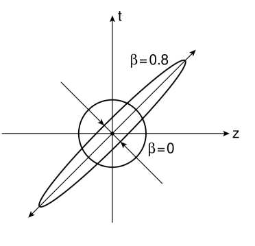
Figure 1: Effect of the Lorentz boost on the space-time wave function. The circular space-time distribution at the rest frame becomes Lorentz-squeezed to become an elliptic distribution. The first version of this figure consists of two ellipses in the 1973 paper by Kim and Noz [27]. This figure consisting of a circle and a ellipse is from the 1978 paper by Kim, Noz, and Oh [43].

Another pressing problem in physics is that hadrons, like the proton, can be regarded as quantum bound states of quarks when they move slowly. However, they appear like collections of partons when they move with velocity very close to that of light [41]. Since the quarks and partons have quite different properties, it is a challenging problem in modern physics to show that they are the same but appear different depending on the observer’s Lorentz frame.

It has been shown that this Lorentz-squeezed wave function can explain the quark model and the parton model as two different manifestations of one covariant entity [44]. Thus, the covariant harmonic oscillator can occupy the third row of Table 1.

The Lorentz-squeezed wave function can be written as

$$\psi_{\eta}(z,t)={1\over\sqrt{\pi}}\exp\left\{-{1\over 4}\left[e^{\eta}(z-t)^{2}+e^{-\eta}(z+t)^{2}\right]\right\}.$$ (131)

As was discussed in the literature for several different purposes [2, 17, 45], this wave function can be expanded as

$$\psi_{\eta}(z,t)={1\over\cosh\eta}\sum_{k}\left(\tanh{\eta\over 2}\right)^{k}\phi_{k}(z)\phi_{k}(t).$$ (132)

This is an expansion in terms of the oscillations along two different directions. If those directions are $x_{1}$ and $x_{2}$, we can write Eq.(132) as

$$\psi_{\eta}(x_{1},x_{2})={1\over\cosh\eta}\sum_{k}\left(\tanh{\eta\over 2}\right)^{k}\phi_{k}(x_{1})\phi_{k}(x_{2}).$$ (133)

The mathematics of harmonic oscillators can be translated into second-quantized Fock space. In the Fock space, this expression describes the two-photon coherent state discussed first by Yuen in 1976 [28].

Appendix B Euler versus Lie Representations

The group $SL(2,c)$ consists of two-by-two unimodular matrices whose elements are complex. There are therefore six independent parameters, and thus six generators of the Lie algebra. This group is locally isomorphic to the six-parameter Lorentz group or $O(3,1)$ applicable to the Minkowskian space of three space-like directions and one time-like direction.

We can construct representations of the group starting from the Lie algebra given in Secs. 2 and 3. We can construct the representation by using a method similar to what Goldstein did for the three-dimensional rotation group in terms of the Euler angles [13]. There are three-generators for the rotation group, but Goldstein starts with rotations around the $z$ and $x$ directions. Rotations around the $y$ axis and the most general form for the rotation matrix can be constructed from repeated applications of those two starting matrices. Let us call this type of approach the “Euler construction.”

In constructing the Lorentz group, we observe first that we need rotations around two different directions. As for the boost, we need boosts along one given direction since boots along other directions can be achieved by rotations.

There are three basic advantages of this approach. First, the number of “starter” matrices is less than the number of generators. For example, we need only two starters for the three-parameter rotation group. In our case, we started with two matrices for the three-parameter group $Sp(2)$ and also for $SU(1,1)$. Second, each starter matrix takes a simple form and has its own physical interpretation.

The third advantage can be stated in the following way. Repeated applications of the starter matrices will lead to a very complicated expression. However, the complicated expression can be decomposed into the minimum number of starter matrices. For example, this number is three for the three-dimensional rotation group. This number is also three for $SU(2)$ and $Sp(2)$. We call this the Euler decomposition. The present paper is based on both the Euler construction and the Euler decomposition.

Among the several useful Euler decompositions, the Iwasawa decomposition plays an important role in the Lorentz group. We have seen in this paper what the decomposition does to the two-by-two matrices of $Sp(2)$, but it has been an interesting subject since Iwasawa’s first publication on this subject [29]. It is beyond the scope of this paper to present a historical review of the subject. However, we would like to point out that there are areas of physics where this important mathematical theorem was totally overlooked.

For instance, in particle theory, Wigner’s little groups dictate the internal space-time symmetries of massive and massless particles which are locally isomorphic to $O(3)$ and $E(2)$ respectively [1]. The little group is the maximal subgroup of the Lorentz group whose transformations do not change the four-momentum of a given particle [34]. The $E(2)$-like subgroup for massless particles is locally isomorphic to the subgroup of $SL(2,c)$ which can be started from one of the matrices in Eq.(149) and the diagonal matrix of Eq.(113). Thus there was an underlying Iwasawa decomposition while the $E(2)$-like subgroup was decomposed into rotation and boost matrices [46], but the authors did not know this.

In optics, there are two-by-two matrices with one vanishing off-diagonal element. It was generally known that this has something to do with the Iwasawa effect, but Simon and Mukunda [47] and Han et al. [4] started treating the Iwasawa decomposition as the main issue in their papers on polarized light.

In para-axial lens optics, the matrices of the form given in Eq.(149) are the starters, and repeated applications of those two starters will lead to the most general form of $Sp(2)$ matrices. It had been a challenging problem since 1985 [35] to write the most general two-by-two matrix in lens optics in terms the minimum number of those starter matrices. This problem has been solved recently [7], and the central issue in the problem was the Iwasawa decomposition.

Appendix C Conjugate Transformations

The core matrix of Eq.(88) contains the chain of the matrices

$$W=\pmatrix{e^{-i\phi}&0\cr 0&e^{i\phi}}\pmatrix{\cosh\eta&\sinh\eta\cr\sinh\eta&\cosh\eta}\pmatrix{e^{-i\xi}&0\cr 0&e^{i\xi}}.$$ (134)

The Lorentz group allows us to simplify this expression under certain conditions.

For this purpose, we transform the above expression into a more convenient form, by taking the conjugate of each of the matrices with

$$C_{1}={1\over\sqrt{2}}\pmatrix{1&i\cr i&1}.$$ (135)

Then $C_{1}WC_{1}^{-1}$ leads to

$$\pmatrix{\cos\phi&-\sin\phi\cr\sin\phi&\cos\phi}\pmatrix{\cosh\eta&\sinh\eta\cr\sinh\eta&\cosh\eta}\pmatrix{\cos\xi&-\sin\xi\cr\sin\xi&\cos\xi}.$$ (136)

In this way, we have converted $W$ of Eq.(134) into a real matrix, but it is not simple enough.

Let us take another conjugate with

$$C_{2}={1\over\sqrt{2}}\pmatrix{1&1\cr-1&1}.$$ (137)

Then the conjugate $C_{2}C_{1}WC_{1}^{-1}C_{2}^{-1}$ becomes

$$\pmatrix{\cos\phi&-\sin\phi\cr\sin\phi&\cos\phi}\pmatrix{e^{\eta}&0\cr 0&e^{-\eta}}\pmatrix{\cos\xi&-\sin\xi\cr\sin\xi&\cos\xi}.$$ (138)

The combined effect of $C_{2}C_{1}$ is

$$C=C_{2}C_{1}={1\over\sqrt{2}}\pmatrix{e^{i\pi/4}&e^{i\pi/4}\cr-e^{-i\pi/4}&e^{-i\pi/4}},$$ (139)

with

$$C^{-1}={1\over\sqrt{2}}\pmatrix{e^{-i\pi/4}&-e^{i\pi/4}\cr e^{-i\pi/4}&e^{i\pi/4}}.$$ (140)

After multiplication, the matrix of Eq.(138) will take the form

$$V=\pmatrix{A&B\cr C&D},$$ (141)

where $A,B,C,$ and $D$ are real numbers. If $B$ and $C$ vanish, this matrix will become diagonal, and the problem will become too simple. If, on the other hand, only one of these two elements become zero, we will achieve a substantial mathematical simplification and will be encouraged to look for physical circumstances which will lead to this simplification.

Let us summarize. We started in this section with the matrix representation $W$ given in Eq.(134). This form can be transformed into the $V$ matrix of Eq.(138) through the conjugate transformation

$$V=CWC^{-1},$$ (142)

where $C$ is given in Eq.(139). Conversely, we can recover the $W$ representation by

$$W=C^{-1}VC.$$ (143)

For calculational purposes, the $V$ representation is much easier because we are dealing with real numbers. On the other hand, the $W$ representation is of the form for the S-matrix we intend to compute. It is gratifying to see that they are equivalent.

Let us go back to Eq.(138) and consider the case where the angles $\phi$ and $\xi$ satisfy the following constraints.

$$\phi+\xi=2\theta,\qquad\phi-\xi=\pi/2,$$ (144)

thus

$$\phi=\theta+\pi/4,\qquad\xi=\theta-\pi/4.$$ (145)

Then in terms of $\theta$, we can reduce the matrix of Eq.(138) to the form

$$\pmatrix{(\cosh\eta)\cos(2\theta)&\sinh\eta-(\cosh\eta)\sin(2\theta)\cr\sinh\eta+(\cosh\eta)\sin(2\theta)&(\cosh\eta)\cos(2\theta)}.$$ (146)

Thus the matrix takes a surprisingly simple form if the parameters $\theta$ and $\eta$ satisfy the constraint

$$\sinh\eta=(\cosh\eta)\sin(2\theta).$$ (147)

Then the matrix becomes

$$\pmatrix{1&0\cr 2\sinh\eta&1}.$$ (148)

This aspect of the Lorentz group is known as the Iwasawa decomposition [29], and has been discussed in the optics literature [4, 11, 47].

Matrices of this form are not so strange in optics. In para-axial lens optics, the translation and lens matrices are written as

$$\pmatrix{1&u\cr 0&1},\quad and\quad\pmatrix{1&0\cr u&1},$$ (149)

respectively. These matrices have the following interesting mathematical property [3],

$$\pmatrix{1&u_{1}\cr 0&1}\pmatrix{1&u_{2}\cr 0&1}=\pmatrix{1&u_{1}+u_{2}\cr 0&1},$$ (150)

and

$$\pmatrix{1&0\cr u_{1}&1}\pmatrix{1&0\cr u_{1}&1}=\pmatrix{1&0\cr u_{1}+u_{2}&1}.$$ (151)

We note that the multiplication is commutative, and the parameter becomes additive. These matrices convert multiplication into addition, as logarithmic functions do.

References

- [1] E. Wigner, Ann. Math. 40, 149 (1939).
- [2] Y. S. Kim and M. E. Noz, Phase Space Picture of Quantum Mechanics (World Scientific, Singapore, 1991).
- [3] D. Han, Y. S. Kim, and M. E. Noz, Phys. Rev. E 56, 6065 (1997).
- [4] D. Han, Y. S. Kim, and M. E. Noz, Phys. Rev. E 60, 1036 (1999).
- [5] M. Born and E. Wolf, Principles of Optics, 6th Ed. (Pergamon, Oxford, 1980).
- [6] C. Brosseau, Fundamentals of Polarized Light (Wiley, New York, 1998).
- [7] S. Baskal and Y. S. Kim, Phys Rev. E 63, 056606 (2001).
- [8] S. Baskal and Y. S. Kim, Phys. Rev. E 67, 056601 (2003).
- [9] S. Baskal and Y. S. Kim, Phys. Rev. E 66, 06604 (2002).
- [10] R. A. M. Azzam and I. Bashara, Ellipsometry and Polarized Light (North-Holland, Amsterdam, 1977).
- [11] E. Georgieva and Y. S. Kim, Phys. Rev. E 64, 026602 (2001).
- [12] E. Georgieva and Y. S. Kim, Phys. Rev. E 68, 026606 (2003).
- [13] H. Goldstein, Classical Mechanics, 2nd Edition (Addison-Wesley, Reading, MA, 1980).
- [14] D. Han, Y. S. Kim, and D. Son, Am. J. Phys. 54, 818 (1986).
- [15] D. Han, Y. S. Kim, and D. Son, J. Math. Phys. 27, 2228 (1986).
- [16] S. Baskal and Y. S. Kim, Europhys. Lett. 40, 375 (1995).
- [17] Y. S. Kim and M. E. Noz, Theory and Applications of the Poincaré Group (Reidel, Dordrecht, 1986).
- [18] A. Janner and T. Janssen, Physica 53, 1 (1971); ibid. 60, 292 (1972).
- [19] Y. S. Kim and E. P. Wigner, J. Math. Phys. 31, 55 (1990).
- [20] S. Weinberg, Phys. Rev. 134, B882 (1964); ibid. 135, B1049 (1964).
- [21] D. Han, Y. S. Kim, and D. Son, Phys. Rev. D 26, 3717 (1982).
- [22] E. Inönü and E. P. Wigner, Proc. Natl. Acad. Sci. (U.S.) 39, 510 (1953).
- [23] H. Bacry and N. P. Chang, Ann. Phys. 47, 407 (1968).
- [24] S. Ferrara and C. Savoy, in Supergravity 1981, S. Ferrara and J. G. Taylor eds. (Cambridge Univ. Press, Cambridge, 1982), p. 151. See also P. Kwon and M. Villasante, J. Math. Phys. 29, 560 (1988); ibid. 30, 201 (1989).
- [25] D. Han, Y. S. Kim, and D. Son, Phys. Lett. B 131, 327 (1983). See also D. Han, Y. S. Kim, M. E. Noz, and D. Son, Am. J. Phys. 52, 1037 (1984).
- [26] Y. S. Kim and E. P. Wigner, J. Math. Phys. 28, 1175 (1987).
- [27] Y. S. Kim and M. E. Noz, Phys. Rev. D 8, 3521 (1973).
- [28] H. P. Yuen, Phys. Rev. A 13, 2226 (1976).
- [29] K. Iwasawa, Ann. Math. 50, 507 (1949).
- [30] Y. S. Kim, J. Opt. B: Quantum Semiclass. Opt. 2, R1 (2000).
- [31] B. C. Sanders and A. Mann, Group 22, Proceedings of the 22nd International Colloquium on Group Theoretical Methods in Physics, S. P. Cornel et al. eds. (International Press, Boston, 1999). See pp 474-478.
- [32] R. A. Campos, B. E. A. Saleh, and M. C. Teich, Phys. Rev. A, 40, 1371 (1989); A. Luis and L. L. Sánchez-Soto, Quantum Semniclass. Opt. 7, 153 (1995).
- [33] R. P. Feynman, Statistical Mechanics (Benjamin/Cummings, Reading, MA, 1972).
- [34] D. Han, Y. S. Kim, and M. E. Noz, Phys. Rev. E 61, 5907 (2000).
- [35] E. C. G. Sudarshan, N. Mukunda, and R. Simon, Optica Acta 32, 855 (1985).
- [36] V. Bargmann, Ann. Math. 48, 568 (1947).
- [37] H. A. Haus, Waves and Fields in Optoelectronics (Prentice-Hall, Englewood Cliffs, New Jersey, 1984).
- [38] J. J. Monzón and L. L. Sánchez-Soto, Am. J. Phys. 64, 156 (1996), J. J. Monzón and L. L. Sánchez-Soto, J. Opt. Soc. Am. A 17, 1475 (2000); J. J. Monzón, T. Yonte, L. L. Sánchez-Soto, and J. Carinena, J. Opt. Soc. Am. A, 19, 985 (2002).
- [39] M. Gell-Mann, Phys. Lett. 13, 598 (1964).
- [40] R. P. Feynman, M. Kislinger, and F. Ravndal, Phys. Rev. D 3, 2706 (1971).
- [41] R. P. Feynman, The Behavior of Hadron Collisions at Extreme Energies, in High Energy Collisions, Proceedings of the Third International Conference, Stony Brook, New York, edited by C. N. Yang et al., Pages 237-249 (Gordon and Breach, New York, 1969).
- [42] P. A. M. Dirac, Rev. Mod. Phys. 21, 392 (1949).
- [43] Y. S. Kim, M. E. Noz, and S. H. Oh, J. Math. Phys. 20, 1342 (1979).
- [44] Y. S. Kim and M. E. Noz, Phys. Rev. D 15, 335 (1977).
- [45] Y. S. Kim, M. E. Noz, and S. H. Oh, Am. J. Phys. 47, 892 (1979).
- [46] D. Han, Y. S. Kim, and D. Son, J. Math. Phys. 28, 2373 (1987).
- [47] R. Simon and N. Mukunda, J. Opt. Soc. Am. 15, 2146 (1998).