Linear optical quantum computing

Abstract

Linear optics with photon counting is a prominent candidate for practical quantum computing. The protocol by Knill, Laflamme, and Milburn [Nature 409, 46 (2001)] explicitly demonstrates that efficient scalable quantum computing with single photons, linear optical elements, and projective measurements is possible. Subsequently, several improvements on this protocol have started to bridge the gap between theoretical scalability and practical implementation. We review the original theory and its improvements, and we give a few examples of experimental two-qubit gates. We discuss the use of realistic components, the errors they induce in the computation, and how these errors can be corrected.

I Quantum computing with light

Quantum computing has attracted much attention over the last ten to fifteen years, partly because of its promise of super-fast factoring and its potential for the efficient simulation of quantum dynamics. There are many different architectures for quantum computers based on many different physical systems. These include atom- and ion-trap quantum computing, superconducting charge and flux qubits, nuclear magnetic resonance, spin- and charge-based quantum dots, nuclear spin quantum computing, and optical quantum computing (for a recent overview see Spiller et al.  2005). All these systems have their own advantages in quantum information processing. However, even though there may now be a few front-runners, such as ion-trap and superconducting quantum computing, no physical implementation seems to have a clear edge over others at this point. This is an indication that the technology is still in its infancy. Quantum computing with linear quantum optics, the subject of this review, has the advantage that the smallest unit of quantum information (the photon) is potentially free from decoherence: The quantum information stored in a photon tends to stay there. The downside is that photons do not naturally interact with each other, and in order to apply two-qubit quantum gates such interactions are essential.

Therefore, if we are to construct an optical quantum computer, one way or another we have to introduce an effective interaction between photons. In section I.4, we review the use of so-called large cross-Kerr nonlinearities to induce a single-photon controlled-NOT operation. However, naturally occurring nonlinearities of this sort are many orders of magnitude smaller than what is needed for our purposes. An alternative way to induce an effective interaction between photons is to make projective measurements with photo-detectors. The difficulty with this technique is that such optical quantum gates are probabilistic: More often than not, the gate fails and destroys the information in the quantum computation. This can be circumvented by using an exponential number of optical modes, but this is by definition not scalable (see also section I.4). In 2001, Knill, Laflamme, and Milburn (KLM 2001) constructed a protocol in which probabilistic two-photon gates are teleported into a quantum circuit with high probability. Subsequent error correction in the quantum circuit is used to bring the error rate down to fault-tolerant levels. We describe the KLM protocol in detail in section II.

Initially, the KLM protocol was designed as a proof that linear optics and projective measurements allow for scalable quantum computing in principle. However, it subsequently spurred on new experiments in quantum optics, demonstrating the operation of high-fidelity probabilistic two-photon gates. On the theoretical front, several improvements of the protocol were proposed, leading to ever smaller overhead cost on the computation. A number of these improvements are based on cluster-state quantum computing, or the one-way quantum computer. Recently, a circuit-based model was shown to have similar scaling properties as the best-known cluster state model. In section III, we describe the several improvements to linear optical quantum information processing in considerable detail, and in section IV, we describe the issues involved in the use of realistic components such as photon detectors, photon sources and quantum memories. Given these realistic components, we discuss loss tolerance and general error correction for Linear Optical Quantum Computing (LOQC) in section V.

We will restrict our discussion to the theory of single-photon implementations of quantum information processors, and we assume some familiarity with the basic concepts of quantum computing. For an introduction to quantum computation and quantum information, see e.g., Nielsen and Chuang (2000). For a review article on optical quantum information processing with continuous variables, see Braunstein and Van Loock (2005). In section VI we conclude with an outlook on other promising optical quantum information processing techniques, such as photonic band-gap structures, weak cross-Kerr nonlinearities, and hybrid matter-photon systems. We start our review with a short introduction to linear optics, $N$ port optical interferometers and circuits, and we define the different versions of the optical qubit.

I.1 Linear quantum optics

The basic building blocks of linear optics are beam splitters, half- and quarter-wave plates, phase shifters, etc. In this section we will describe these devices mathematically and establish the convention that is used throughout the rest of the paper.

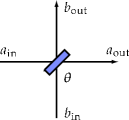
Figure 1: The beam splitter with transmission amplitude $\cos\theta$.

The quantum-mechanical plane-wave expansion of the electromagnetic vector potential is usually expressed in terms of the annihilation operators $\hat{a}_{j}(k)$ and their adjoints, the creation operators:

$$A^{\mu}(x,t)=\int\frac{d^{3}k}{2\omega_{k}}\sum_{j=1,2}\epsilon^{\mu}_{j}(k)\,\hat{a}_{j}(k)\,e^{ikx-i\omega_{k}t}+\text{H.c.,}$$

where $j$ indexes the polarisation in the Coulomb gauge and $\epsilon^{\mu}_{j}$ is the corresponding polarisation vector. For the moment we suppress the polarisation degree of freedom and consider general properties of the creation and annihilation operators. They bear their names because they act in a specific way on the Fock states $|n\rangle$:

$$\hat{a}|n\rangle=\sqrt{n}|n-1\rangle\quad\text{and}\quad\hat{a}^{\dagger}|n\rangle=\sqrt{n+1}|n+1\rangle\;,$$ (1)

where we suppressed the $k$ dependence. It is straightforward to show that $\hat{n}(k)\equiv\hat{a}^{\dagger}(k)\hat{a}(k)$ is the number operator $\hat{n}|n\rangle=n|n\rangle$ for a given mode with momentum $k$. The canonical commutation relations between $\hat{a}$ and $\hat{a}^{\dagger}$ are given by

$$\left[\hat{a}(k),\hat{a}^{\dagger}(k^{\prime})\right] = \delta(k-k^{\prime})$$ (2)

$$\left[\hat{a}(k),\hat{a}(k^{\prime})\right] = \left[\hat{a}^{\dagger}(k),\hat{a}^{\dagger}(k^{\prime})\right]=0\;.$$ (3)

In the rest of this review, we denote the information about the spatial mode, $k$, by a subscript, since we will not be concerned with the geometrical details of the interferometers we describe, only how the spatial modes are connected. Also, to avoid notational clutter we will use operator hats only for non-unitary and non-Hermitian operators, as well as cases where omission of the hat would lead to confusion.

An important optical component is the single-mode phase shift. It changes the phase of the electromagnetic field in a given mode:

$$\hat{a}^{\dagger}_{\rm out}=e^{i\phi\hat{a}_{\rm in}^{\dagger}\hat{a}_{\rm in}}\,\hat{a}_{\rm in}^{\dagger}\,e^{-i\phi\hat{a}_{\rm in}^{\dagger}\hat{a}_{\rm in}}=e^{i\phi}\hat{a}_{\rm in}^{\dagger}\;,$$ (4)

with the interaction Hamiltonian $H_{\varphi}=\phi\,\hat{a}_{\rm in}^{\dagger}\hat{a}_{\rm in}$ (here, and throughout this review, we use the convention that $\hbar=1$, and the time dependence is absorbed in $\phi$). This Hamiltonian is proportional to the number operator, which means that the photon number is conserved. Physically, a phase shifter is a slab of transparent material with an index of refraction that is different from that of free space.

Another important component is the beam splitter (see Fig. 1). Physically, it consists of a semi-reflective mirror: when light falls on this mirror, part will be reflected and part will be transmitted. The theory of the lossless beam splitter is central to LOQC, and was developed by Zeilinger (1981) and Fearn and Loudon (1987) . Lossy beam splitters were studied by Barnett et al. (1989) . The transmission and reflection properties of general dielectric media were studied by Dowling (1998). Let the two incoming modes on either side of the beam splitter be denoted by $\hat{a}_{\rm in}$ and $\hat{b}_{\rm in}$, and the outgoing modes by $\hat{a}_{\rm out}$ and $\hat{b}_{\rm out}$. When we parameterise the probability amplitudes of these possibilities as $\cos\theta$ and $\sin\theta$, and the relative phase as $\varphi$, then the beam splitter yields an evolution in operator form

$$\hat{a}_{\rm out}^{\dagger} = \cos\theta\,\hat{a}_{\rm in}^{\dagger}+ie^{-i\varphi}\sin\theta\,\hat{b}_{\rm in}^{\dagger}\;,$$ (5)

$$\hat{b}_{\rm out}^{\dagger} = ie^{i\varphi}\sin\theta\,\hat{a}_{\rm in}^{\dagger}+\cos\theta\,\hat{b}_{\rm in}^{\dagger}\;,$$ (6)

The reflection and transmission coefficients $R$ and $T$ of the beam splitter are $R=\sin^{2}\theta$ and $T=1-R=\cos^{2}\theta$. The relative phase shift $ie^{\pm i\varphi}$ ensures that the transformation is unitary. Typically, we choose either $\varphi=0$ or $\varphi=\pi/2$. Mathematically, the two parameters $\theta$ and $\varphi$ represent the angles of a rotation about two orthogonal axes in the Poincaré sphere. The physical beam splitter can be described by any choice of $\theta$ and $\varphi$, provided the correct phase shifts are applied to the outgoing modes.

In general the Hamiltonian $H_{\rm BS}$ of the beam splitter evolution in Eq. (5) is given by

$$H_{\rm BS}=\theta e^{i\varphi}\hat{a}_{\rm in}^{\dagger}\hat{b}_{\rm in}+\theta e^{-i\varphi}\hat{a}_{\rm in}\hat{b}_{\rm in}^{\dagger}\;.$$ (7)

Since the operator $H_{\rm BS}$ commutes with the total number operator, $[H_{\rm BS},\hat{n}]=0$, the photon number is conserved in the lossless beam splitter, as one would expect.

The same mathematical description applies to the evolution due to a polarisation rotation, physically implemented by quarter- and half-wave plates. Instead of having two different spatial modes $a_{\rm in}$ and $b_{\rm in}$, the two incoming modes have different polarisations. We write $\hat{a}_{\rm in}\rightarrow\hat{a}_{x}$ and $\hat{b}_{\rm in}\rightarrow\hat{a}_{y}$ for some orthogonal set of coordinates $x$ and $y$ (i.e., $\langle x|y\rangle=0$). The parameters $\theta$ and $\varphi$ are now angles of rotation:

$$\hat{a}_{x^{\prime}}^{\dagger} = \cos\theta\,\hat{a}_{x}^{\dagger}+ie^{-i\varphi}\sin\theta\,\hat{a}_{y}^{\dagger}\;,$$ (8)

$$\hat{a}_{y^{\prime}}^{\dagger} = ie^{i\varphi}\sin\theta\,\hat{a}_{x}^{\dagger}+\cos\theta\,\hat{a}_{y}^{\dagger}\;.$$ (9)

This evolution has the same Hamiltonian as the beam splitter, and it formalises the equivalence between the so-called polarisation and dual-rail logic. These transformations are sufficient to implement any photonic single-qubit operation Simon and Mukunda (1990).

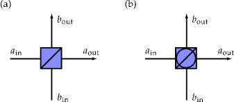
Figure 2: The polarising beam splitter cut to different polarisation bases. (a) The horizontal-vertical basis. (b) The diagonal basis.

The last linear optical element that we highlight here is the polarising beam splitter (PBS). In circuit diagrams, it is usually drawn as a box around a regular beam splitter (see Fig. 2a). If the PBS is cut to separate horizontal and vertical polarisation, the transformation of the incoming modes ($a_{\rm in}$ and $b_{\rm in}$) yields the following outgoing modes (($a_{\rm out}$ and $b_{\rm out}$):

$$\hat{a}_{{\rm in},H}\rightarrow\hat{a}_{{\rm out},H} \hat{a}_{{\rm in},V}\rightarrow\hat{b}_{{\rm out},V}$$ and (10)

$$\hat{b}_{{\rm in},H}\rightarrow\hat{b}_{{\rm out},H} \hat{b}_{{\rm in},V}\rightarrow\hat{a}_{{\rm out},V}$$ and (11)

We can also cut the PBS to different polarisation directions (e.g., $L$ and $R$), in which case we make the substitution $H\leftrightarrow L$, $V\leftrightarrow R$. Diagrammatically a PBS cut with a different polarisation usually has a circle drawn inside the box (Fig. 2b).

At this point, we should devote a few words to the term “linear optics”. Typically this denotes the set of optical elements whose interaction Hamiltonian is bilinear in the creation and annihilation operators:

$$H=\sum_{jk}A_{jk}\hat{a}_{j}^{\dagger}\hat{a}_{k}\;.$$ (12)

An operator of this form commutes with the total number operator, and has the property that a simple mode transformation of creation operators into a linear combination of other creation operators affects only the matrix $A$, but does not introduce terms that are quadratic (or higher) in the creation or annihilation operators. However, from a field-theoretic point of view, the most general linear Bogoliubov transformation of creation and annihilation operators is given by

$$\hat{a}_{j}\rightarrow\sum_{k}u_{jk}\hat{a}_{k}+v_{jk}\hat{a}_{k}^{\dagger}\;.$$ (13)

Clearly, when such a transformation is substituted in Eq. (12) this will give rise to terms such as $\hat{a}_{j}\hat{a}_{k}$ and $\hat{a}_{j}^{\dagger}\hat{a}_{k}^{\dagger}$, i.e., squeezing. The number of photons is not conserved in such a process. For the purpose of this review, we exclude squeezing as a resource other than as a method for generating single photons.

With the linear optical elements introduced in this section we can build large optical networks. In particular, we can make computational circuits by using known states as the input and measuring the output states. Next we will study these optical circuits in more detail.

I.2 $N$ port interferometers and optical circuits

An optical circuit can be thought of as a black box with incoming and outgoing modes of the electromagnetic field. The black box transforms a state of the incoming modes into a different state of the outgoing modes. The modes might be mixed by beam splitters, or they may pick up a relative phase shift or polarisation rotation. These operations all belong to a class of optical components that preserve the photon number, as described in the previous section. In addition, the box may include measurement devices, the outcomes of which may modify optical components on the remaining modes. This is called feed-forward detection, and it is an important technique that can increase the efficiency of a device Lapaire et al. (2003); Clausen et al. (2003).

Optical circuits can also be thought of as a general unitary transformation on $N$ modes, followed by the detection of a subset of these modes (followed by unitary transformation on the remaining modes, detection, and so on). The interferometric part of this circuit is also called an $N$ port interferometer. $N$ ports yield a unitary transformation $U$ of the spatial field modes $a_{k}$, with $j,k\in\{1,\ldots,N\}$:

$$\hat{b}_{k}\rightarrow\sum_{j=1}^{N}U_{jk}\hat{a}_{j}\qquad\mbox{and}\qquad\hat{b}^{\dagger}_{k}\rightarrow\sum_{j=1}^{N}U_{jk}^{*}\hat{a}^{\dagger}_{j}\;,$$ (14)

where the incoming modes of the $N$ port are denoted by $a_{j}$ and the outgoing modes by $b_{j}$. The explicit form of $U$ is given by the repeated application of transformations such as given in Eqs. (4), (5), and (8).

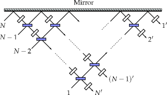
Figure 3: Decomposing an $N$ port unitary $U(N)$ into $SU(2)$ group elements, i.e., beam splitters and phase shifters. Moreover, this is an efficient process: the maximum number of beam splitters needed is $N(N-1)/2$.

The two-mode operators $\hat{L}_{+}=\hat{a}^{\dagger}\hat{b}$, $\hat{L}_{-}=\hat{a}\hat{b}^{\dagger}$, and $\hat{L}_{0}=(\hat{a}^{\dagger}\hat{a}-\hat{b}^{\dagger}\hat{b})/2$ form an $su(2)$ Lie algebra:

$$[\hat{L}_{0},\hat{L}_{\pm}]=\pm\hat{L}_{\pm}\quad\mbox{and}\quad[\hat{L}_{+},\hat{L}_{-}]=2\hat{L}_{0}\;.$$ (15)

This means that any two-mode interferometer exhibits $U(2)$ symmetry. In general, an $N$ port interferometer can be described by a transformation from the group $U(N)$. Reck et al. (1994) demonstrated that the converse is also true, i.e., that any unitary transformation of $N$ optical modes can be implemented efficiently with an $N$ port interferometer . They showed how a general $U(N)$ element can be broken down into $SU(2)$ elements, for which we have a complete physical representation in terms of beam splitters and phase shifters (see Fig. 3). The primitive element is a matrix $T_{pq}$ defined on the modes $p$ and $q$, which corresponds to a beam splitter and phase shifts. Implicit in this notation is the identity operator on the rest of the optical modes, such that $T_{pq}\equiv T_{pq}\otimes\mbox{\small 1}\!\!\mbox{1}_{\rm rest}$. We then have

$$U(N)\cdot T_{N,N-1}\cdots T_{N,1}=U(N-1)\oplus e^{i\phi}\;,$$ (16)

where $\phi$ is a single-mode phase. Concatenating this procedure leads to a full decomposition of $U(N)$ into $T$ elements, which in turn are part of $SU(2)$. The maximum number of beam splitter elements $T$ that are needed is $N(N-1)/2$. This procedure is thus manifestly scalable.

Subsequently, it was shown by Törmä et al. (1995, 1996) and Jex et al. (1995) how one can construct multi-mode Hamiltonians that generate these unitary mode-transformations, and a three-path Mach-Zehnder interferometer was demonstrated experimentally by Weihs et al. (1996). A good introduction to linear optical networks is given by Leonhardt (2003) and a determination of effective Hamiltonians is given by Leonhardt and Neumaier (2004). For a treatment of optical networks in terms of their permanents, see Scheel (2004). Optical circuits in a (general) relativistic setting are described by Kok and Braunstein (2006).

I.3 Qubits in linear optics

Formally, a qubit is a quantum system with an $SU(2)$ symmetry. We saw above that two optical modes form a natural implementation of this symmetry. In general, two modes with fixed total photon number $n$ furnish natural irreducible representations of this group with the dimension of the representation given by $n+1$ Biedenharn and Louck (1981). It is at this point not specified whether we should use spatial or polarisation modes. In linear optical quantum computing, the qubit of choice is usually taken to be a single photon that has the choice of two different modes $|0\rangle_{L}=|1\rangle\otimes|0\rangle\equiv|1,0\rangle$ and $|1\rangle_{L}=|0\rangle\otimes|1\rangle\equiv|0,1\rangle$. This is called a dual-rail qubit. When the two modes represent the internal polarisation degree of freedom of the photon ($|0\rangle_{L}=|H\rangle$ and $|1\rangle_{L}=|V\rangle$), we speak of a polarisation qubit. In this review we will reserve the term “dual rail” for a qubit with two spatial modes. As we showed earlier, these two representations are mathematically equivalent, and we can physically switch between them using polarisation beam splitters. In addition, some practical applications (typically involving a dephasing channel such as a fibre) may call for so-called time-bin qubits, in which the two computational qubit values are “early” and “late” arrival times in a detector. However, this degree of freedom does not exhibit a natural internal $SU(2)$ symmetry: Arbitrary single-qubit operations are very difficult to implement. In this review we will be concerned mainly with polarisation and dual-rail qubits.

In order to build a quantum computer, we need both single-qubit operations as well as two-qubit operations. Single-qubit operations are generated by the Pauli operators $\sigma_{x}$, $\sigma_{y}$, and $\sigma_{z}$, in the sense that the operator $\exp(i\theta\sigma_{j})$ is a rotation about the $j$-axis in the Bloch sphere with angle $\theta$. As we have seen, these operations can be implemented with phase shifters, beam splitters, and polarisation rotations on polarisation and dual-rail qubits. In this review, we will use the convention that $\sigma_{x}$, $\sigma_{y}$, and $\sigma_{z}$ denote physical processes, while we use $X$, $Y$, and $Z$ for the corresponding logical operations on the qubit. These two representations become inequivalent when we deal with logical qubits that are encoded in multiple physical qubits.

Whereas single-qubit operations are straightforward in the polarisation and dual-rail representation, the two-qubit gates are more problematic. Consider, for example, the transformation from a state in the computational basis to a maximally entangled Bell state:

$$|H,H\rangle_{ab}~{}\rightarrow~{}\frac{1}{\sqrt{2}}\left(|H,V\rangle_{cd}+|V,H\rangle_{cd}\right)\;.$$ (17)

This is the type of transformation that requires a two-qubit gate. In terms of the creation operators (and ignoring normalisation), the linear optical circuit that is supposed to create Bell states out of computational basis states is described by a Bogoliubov transformation of both creation operators

$$\hat{a}_{H}^{\dagger}\hat{b}_{H}^{\dagger} \rightarrow \left(\sum_{k=H,V}\alpha_{k}\hat{c}_{k}^{\dagger}+\beta_{k}\hat{d}_{k}^{\dagger}\right)\left(\sum_{k=H,V}\gamma_{k}\hat{c}_{k}^{\dagger}+\delta_{k}\hat{d}_{k}^{\dagger}\right)$$ (18)

$$\neq \hat{c}_{H}^{\dagger}\hat{d}_{V}^{\dagger}+\hat{c}_{V}^{\dagger}\hat{d}_{H}^{\dagger}\;.$$ (19)

It is immediately clear that the right-hand sides in both lines cannot be made the same for any choice of $\alpha_{k}$, $\beta_{k}$, $\gamma_{k}$, and $\delta_{k}$: The top line is a separable expression in the creation operators, while the bottom line is an entangled expression in the creation operators. Therefore, linear optics alone cannot create maximal polarisation entanglement from single polarised photons in a deterministic manner Kok and Braunstein 2000a . Entanglement that is generated by changing the definition of our subsystems in terms of the global field modes is inequivalent to the entanglement that is generated by applying true two-qubit gates to single-photon polarisation or dual-rail qubits.

Note also that if we choose our representation of the qubit differently, we can implement a two-qubit transformation. Consider the single-rail qubit encoding $|0\rangle_{L}=|0\rangle$ and $|1\rangle_{L}=|1\rangle$. That is, the qubit is given by the vacuum and the single-photon state. We can then implement the following (unnormalised) transformation deterministically:

$$|1,0\rangle~{}\rightarrow~{}|1,0\rangle+|0,1\rangle\;.$$ (20)

This is a 50:50 beam splitter transformation. However, in this representation the single-qubit operations cannot be implemented deterministically with linear optical elements, since these transformations do not preserve the photon number Paris (2000). This implies that we cannot implement single-qubit and two-qubit gates deterministically for the same physical representation. For linear optical quantum computing, we typically need the ability to (dis-) entangle field modes. We therefore have to add a non-linear component to our scheme. Two possible approaches are the use of Kerr nonlinearities, which we briefly review in the next section, and the use of projective measurements. In the rest of this review, we concentrate mainly on linear optical quantum computing with projective measurements, based on the work by Knill, Laflamme, and Milburn.

Finally, in order to make a quantum computer with light that can outperform any classical computer, we need to understand more about the criteria that make quantum computers “quantum”. For example, some simple schemes in quantum communication require only superpositions of quantum states to distinguish them from their corresponding classical ones. However, we know that this is not sufficient for general computational tasks.

First, we give two definitions. The Pauli group $P$ is the set of Pauli operators with coefficients $\{\pm 1,\pm i\}$. For instance, the Pauli group for one qubit is $\{\mbox{\small 1}\!\!\mbox{1},\pm X,\pm Y,\pm Z,\pm i\mbox{\small 1}\!\!\mbox{1}\pm iX,\pm iY,\pm iZ,\}$ where 11 is the identity matrix. The Pauli group for $n$ qubits consists of elements that are products of $n$ Pauli operators, including the identity. In addition, we define the Clifford group $C$ of transformations that leave the Pauli group invariant. In other words, for any element of the Clifford group $c$ and any element of the Pauli group $p$, we have

$$cpc^{\dagger}=p^{\prime}\quad\text{with}\quad p^{\prime}\in P\;.$$ (21)

Prominent members of the Clifford group are the Hadamard transformation, phase transformations, and the controlled-not (CNOT) Note that the Pauli group is a subgroup of the Clifford group.

The Gottesman-Knill theorem (1999) states that any quantum algorithm that initiates in the computational basis and employs only transformations (gates) from the the Clifford group, along with projective measurements in the computational basis, can be efficiently simulated on a classical computer. This means there is no computational advantage in restricting the quantum computer to such circuits. A classical machine could simulate them efficiently.

In discrete-variable quantum information processing, the Gottesman-Knill theorem provides a valuable tool for assessing the classical complexity of a given process. (For a precise formulation and proof of this theorem, see Nielsen and Chuang, page 464). Although the set of gates in the Pauli and Clifford groups does not satisfy the universality requirements, the addition of a single-qubit $\pi/8$ gate will render the set universal. In single-photon quantum information processing we have easy access to such single-qubit operations.

I.4 Early optical quantum computers and nonlinearities

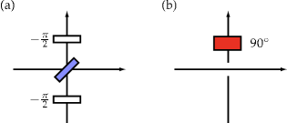
Figure 4: Linear optical quantum computing simulation according to Cerf, Adami, and Kwiat. (a) Hadamard gate. (b) CNOT gate. The four two-qubit degrees of freedom are carried by which-path and polarization information. The broken line indicates that there is no interaction between the crossing modes.

Before the work of Knill, Laflamme, and Milburn (KLM), quantum information processing with linear optics was studied (among other things) in non-scalable architectures by Cerf, Adami, and Kwiat (1998, 1999). Their linear optical protocol can be considered a simulation of a quantum computer: $n$ qubits are represented by a single photon in $2^{n}$ different paths. In such an encoding, both single- and two-qubit gates are easily implemented using (polarisation) beam splitters and phase shifters. For example, let a single qubit be given by a single photon in two optical modes: $|0\rangle_{L}=|1,0\rangle$ and $|1\rangle_{L}=|0,1\rangle$. The Hadamard gate acting on this qubit can then be implemented with a 50:50 beam splitter given by Eq. (5) with $\varphi=0$, and two $-\pi/2$ phase shifters (see Fig. 4a):

$$|1,0\rangle \rightarrow |1,0\rangle+i|0,1\rangle\rightarrow|1,0\rangle+|0,1\rangle$$

$$|0,1\rangle \rightarrow -i\left(i|1,0\rangle+|0,1\rangle\right)\rightarrow|1,0\rangle-|0,1\rangle_{\rm out}\;,$$ (22)

where we suppressed the normalisation.

The CNOT gate in the Cerf, Adami, and Kwiat protocol is even simpler: suppose that the two optical modes in Fig. 4b carry polarisation. The spatial degree of freedom carries the control qubit, and the polarisation carries the target. If the photon is in the vertical spatial mode, it will undergo a polarisation rotation; thus implementing a CNOT. The control and target qubits can be interchanged trivially using a polarisation beam splitter.

Since this protocol requires an exponential number of optical modes, this is a simulation rather than a fully scalable quantum computer. Other proposals in the same spirit include work by Clauser and Dowling (1996), Summhammer (1997), Spreeuw (1998), and Ekert (1998). Using this simulation, a classical version of Grover’s search algorithm can be implemented Kwiat et al. (2000). General quantum logic using polarised photons was studied by Törmä and Stenholm (1996), Stenholm (1996), and Franson and Pittman (1999).

Prior to KLM, it was widely believed that scalable all-optical quantum computing needed a nonlinear component, such as a Kerr medium. These media are typically characterised by a refractive index $n_{\rm Kerr}$ that has a nonlinear component:

$$n_{\rm Kerr}=n_{0}+\chi^{(3)}E^{2}\;.$$ (23)

Here, $n_{0}$ is the ordinary refractive index, and $E^{2}$ is the optical intensity of a probe beam with proportionality constant $\chi^{(3)}$. A beam traversing through a Kerr medium will then experience a phase shift that is proportional to its intensity.

A variation on this is the cross-Kerr medium, in which the phase shift of a signal beam is proportional to the intensity of a second probe beam. In the language of quantum optics, we describe the cross-Kerr medium by the Hamiltonian

$$H_{\rm Kerr}=\kappa\,\hat{n}_{s}\hat{n}_{p}\;,$$ (24)

where $\hat{n}_{s}$ and $\hat{n}_{p}$ are the number operators for the signal and probe mode, respectively. Compare $H_{\rm Kerr}$ with the argument of the exponential in Eq. (4): Transforming the probe (signal) mode using this Hamiltonian induces a phase shift that depends on the number of photons in the signal (probe) mode. Indeed, the mode transformations of the signal and probe beams are

$$\hat{a}_{s}\rightarrow\hat{a}_{s}e^{-i\tau\hat{n}_{p}}\quad\text{and}\quad\hat{a}_{p}\rightarrow\hat{a}_{p}e^{-i\tau\hat{n}_{s}}\;,$$ (25)

with $\tau\equiv\kappa t$. When the cross-Kerr medium is placed in one arm of a balanced Mach-Zehnder interferometer, a sufficiently strong phase shift $\tau$ can switch the field from one output mode to another (see Fig. 5a). For example, if the probe beam is a (weak) optical field, and the signal mode may or may not be populated with a single photon, then the detection of the output ports of the Mach-Zehnder interferometer reveals whether there was a photon in the signal beam. Moreover, we obtain this information without destroying the signal photon. This is called a quantum non-demolition measurement Imoto et al. (1985).

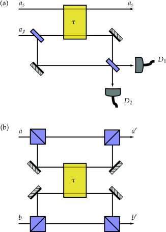
Figure 5: Using cross-Kerr nonlinearities ($\tau$) in optical information processing. (a) Single-photon quantum non-demolition measurement. The Mach-Zehnder interferometer is balanced, such that the presence of a photon in the signal mode directs the probe field to the dark output port. (b) Single-photon CZ gate. When both photons in modes $a$ and $b$ are vertically polarised, the two-photon state acquires a relative phase. This results in an entangling gate that, together with single-photon rotations, is sufficient for universal quantum computing.

It is not hard to see that we can use this mechanism to create an all-optical CZ gate for photonic qubits [for the definition of a CZ gate, see Eq. (39a)]. Such a gate would give us the capability to build an all-optical quantum computer. Let’s assume that our qubit states are single photons with horizontal or vertical polarisation. In Fig. 5b, we show how the cross-Kerr medium should be placed. The mode transformations are

$$\hat{a}_{H}\hat{b}_{H}\rightarrow\hat{a}_{H}^{\prime}\hat{b}_{H}^{\prime} \hat{a}_{V}\hat{b}_{H}\rightarrow\hat{a}_{V}^{\prime}\hat{b}_{H}^{\prime}$$ (26)

$$\hat{a}_{H}\hat{b}_{V}\rightarrow\hat{a}_{H}^{\prime}\hat{b}_{V}^{\prime} \hat{a}_{V}\hat{b}_{V}\rightarrow\hat{a}_{V}^{\prime}\hat{b}_{V}^{\prime}\,e^{i\tau}\;,$$ (27)

which means that the strength of the Kerr nonlinearity should be $\tau=\pi$ in order to implement a CZ gate. It is trivial to transform this gate into a CNOT gate. A Kerr-based Fredkin gate was developed by Yamamoto al. (1988) and Milburn (1989). Architectures based on these or similar nonlinear optical gates were studied by Chuang and Yamamoto (1995), Howell and Yeazell (2000b, 2000c), and d’Ariano et al. (2000). Nonlinear interferometers are treated in Sanders and Rice (2000), while state transformation using Kerr media is the subject of Clausen et al. (2002). Recently, Hutchinson and Milburn (2004) proposed cross-Kerr nonlinearities to create cluster states for quantum computing. We will discuss cluster state quantum computing in some detail in section III.1.

Unfortunately, even the largest natural cross-Kerr nonlinearities are extremely weak ($\chi^{(3)}\approx 10^{-22}$ m²V^-2). Operating in the optical single-photon regime with a mode volume of approximately 0.1 cm³, the Kerr phase shift is only $\tau\approx 10^{-18}$ Kok et al. (2002). This makes Kerr-based optical quantum computing extremely challenging, if not impossible. Much larger cross-Kerr nonlinearities of $\tau\approx 10^{-5}$ can be obtained with electromagnetically-induced transparent materials Schmidt and Imamoǧlu (1996). However, this value of $\tau$ is still much too small to implement the gates we discussed above. Towards the end of this review we will indicate how such small-but-not-tiny cross-Kerr nonlinearities may be used for quantum computing.

Turchette et al. (1995) proposed a different method of inducing a phase shift when a signal mode $s$ and probe mode $p$ of different frequency are both populated by a single polarised photon. By sending both modes through a cavity containing caesium atoms, they obtain a phase shift that is dependent on the polarisations of the input modes:

$$|L,L\rangle_{sp} \rightarrow |L,L\rangle_{sp}$$ (28)

$$|R,L\rangle_{sp} \rightarrow e^{i\phi_{s}}|R,L\rangle_{sp}$$ (29)

$$|L,R\rangle_{sp} \rightarrow e^{i\phi_{p}}|L,R\rangle_{sp}$$ (30)

$$|R,R\rangle_{sp} \rightarrow e^{i(\phi_{s}+\phi_{p}+\delta)}|R,R\rangle_{sp},$$ (31)

where $|L\rangle=|H\rangle+i|V\rangle$ and $|R\rangle=|H\rangle-i|V\rangle$. Using weak coherent pulses, Turchette et al. found $\phi_{s}=17.5^{\circ}\pm 1$, $\phi_{p}=12.5^{\circ}\pm 1$, and $\delta=16^{\circ}\pm 3$. An improvement of this system was proposed by Hofmann et al. (2003). These authors showed how a phase shift of $\pi$ can be achieved with a single two-level atom in a one-sided cavity. The cavity effectively enhances the tiny nonlinearity of the atom. The losses in this system are negligible.

In section VI we will return to systems in which (small) phase shifts can be generated using nonlinear optical interactions, but the principal subject of this review is how projective measurements can induce enough of a nonlinearity to make linear optical quantum computing possible.

II A new paradigm for optical quantum computing

In 2000, Knill, Laflamme, and Milburn proved that it is indeed possible to create universal quantum computers with linear optics, single photons, and photon detection Knill et al. (2001). They constructed an explicit protocol, involving off-line resources, quantum teleportation, and error correction. In this section, we will describe this new paradigm, which has become known as the KLM scheme, starting from the description of linear optics that we developed in the previous section. In sections II.1, II.2 and II.3, we introduce some elementary probabilistic gates and their experimental realizations, followed by a characterisation of gates in section II.4, and a general discussion on nonlinear unitary gates with projective measurements in section II.5. We then describe how to teleport these gates into an optical computational circuit in sections II.6 and II.7, and the necessary error correction is outlined in section II.8. Recently, Myers and Laflamme (2005) published a tutorial on the original “KLM theory.”

II.1 Elementary gates

Physically, the reason why we cannot construct deterministic two-qubit gates in the polarisation and dual-rail representation, is that photons do not interact with each other. The only way in which photons can directly influence each other is via the bosonic symmetry relation. Indeed, linear optical quantum computing exploits exactly this property, i.e., the bosonic commutation relation $[\hat{a},\hat{a}^{\dagger}]=1$. To see what we mean by this statement, consider two photons in separate spatial modes interacting on a 50:50 beam splitter. The transformation will be

$$|1,1\rangle_{ab} = \hat{a}^{\dagger}\hat{b}^{\dagger}|0\rangle$$ (32)

$$\rightarrow \frac{1}{2}\left(\hat{c}^{\dagger}+\hat{d}^{\dagger}\right)\left(\hat{c}^{\dagger}-\hat{d}^{\dagger}\right)|0\rangle_{cd}$$ (33)

$$= \frac{1}{2}\left(\hat{c}^{\dagger 2}-\hat{d}^{\dagger 2}\right)|0\rangle_{cd}$$ (34)

$$= \frac{1}{\sqrt{2}}\left(|2,0\rangle_{cd}-|0,2\rangle_{cd}\right)\;.$$ (35)

It is clear (from the second and third line) that the bosonic nature of the electromagnetic field gives rise to photon bunching: the incoming photons pair off together. This is a strictly quantum-mechanical effect, since classically, the two photons could equally well end up in different output modes. In terms of quantum interference, there are two paths leading from the input state $|1,1\rangle_{\rm in}$ to the output state $|1,1\rangle_{\rm out}$: Either both photons are transmitted, or both photons are reflected. The relative phases of these paths are determined by the beam splitter equation (5):

$$|1,1\rangle_{\rm in} \rightarrow_{\rm trans.} \cos^{2}\theta\,|1,1\rangle_{\rm out},$$ (36)

$$|1,1\rangle_{\rm in} \rightarrow_{\rm refl.} -\sin^{2}\theta\,e^{i\varphi}e^{-i\varphi}|1,1\rangle_{\rm out}.$$ (37)

For a 50:50 beam splitter, we have $\cos^{2}\theta=\sin^{2}\theta=1/2$, and the two paths cancel exactly, irrespective of the value of $\varphi$.

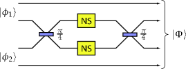
Figure 6: The conditional phase gate (CZ). This gate uses two NS gates to change the relative phase of the two qubits: when both qubits are in the $|1\rangle$ state, the two photons interfere on the 50:50 beam splitter ($\cos^{2}(\pi/4)=1/2$). The Hong-Ou-Mandel effect then ensures that both photons exit the same output mode, and the NS gates induce a relative phase $\pi$. Upon recombination on the second beam splitter, this phase shows up only in the states where both qubits were in the $|1\rangle$ state.

The absence of the $|1,1\rangle_{cd}$ term is called the Hong-Ou-Mandel effect Hong et al. (1987), and it lies at the heart of linear optical quantum computing. However, as we have argued in section I.3, this is not enough to make deterministic linear optical quantum computing possible, and we have to turn our attention instead to probabilistic gates.

As was shown by Lloyd (1995), almost any two-qubit gate is universal for quantum computing (in addition to single-qubit gates), but in linear optics we usually consider the controlled-phase gate (CZ, also sometimes known as CPHASE or CSign) and the controlled-not gate (CNOT). In terms of a truth table, they induce the following transformations

 Control  Target  CZ  CNOT

$$|0\rangle$$

(38)

which is identical to

$$|q_{1},q_{2}\rangle ~{}\rightarrow_{\rm CZ}~{} (-1)^{q_{1}q_{2}}|q_{1},q_{2}\rangle$$ (39a)

$$|q_{1},q_{2}\rangle ~{}\rightarrow_{\rm CNOT}~{} |q_{1},q_{2}\oplus q_{1}\rangle\;.$$ (39b)

Here $q_{k}$ takes the qubit values 0 and 1, while $q_{2}\oplus q_{1}$ is taken modulo 2.

A CZ gate can be constructed in linear optics using two nonlinear sign (NS) gates. The NS gate acts on the three lowest Fock states in the following manner:

$$\alpha|0\rangle+\beta|1\rangle+\gamma|2\rangle~{}\rightarrow~{}\alpha|0\rangle+\beta|1\rangle-\gamma|2\rangle\;.$$ (40)

Its action on higher number states is irrelevant, as long as it does not change the amplitudes of $|0\rangle$, $|1\rangle$, or $|2\rangle$. Consider the optical circuit drawn in Fig. 6, and suppose the (separable) input state is given by $|\phi_{1}\rangle\otimes|\phi_{2}\rangle=(\alpha|0,1\rangle+\beta|1,0\rangle)(\gamma|0,1\rangle+\delta|1,0\rangle)$. Subsequently, we apply the beam splitter transformation to the first and third mode, and find the Hong-Ou-Mandel effect only when both modes are populated by one photon. The NS gates will then induce a phase shift of $\pi$. Applying a second beam splitter operation yields

$$|\Phi\rangle = \alpha\gamma|0,1,0,1\rangle+\alpha\delta|0,1,1,0\rangle$$ (42)

$$+\beta\gamma|1,0,0,1\rangle-\beta\delta|1,0,1,0\rangle\;.$$

This is no longer separable in general. In fact, when we choose $\alpha=\beta=\gamma=\delta=1/\sqrt{2}$, then the output state is a maximally entangled state. The overall probability of this CZ gate $p_{CZ}=p_{NS}^{2}$.

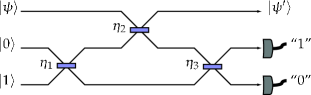
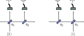
Figure 7: The nonlinear sign (NS) gate according to Knill, Laflamme and Milburn. The beam splitter transmission amplitudes are $\eta_{1}=\eta_{3}=1/(4-2\sqrt{2})$ and $\eta_{2}=3-2\sqrt{2}$.

Figure 8: The two equivalent versions of the NS gate by Ralph et al. (2002b). Only two beam splitters are used, while the other resources are identical to the NS gate by Knill. Laflamme and Milburn. The success probability of this gate is $(3-\sqrt{2})/7$.

It is immediately clear that we cannot make the NS gate with a regular phase shifter, because only the state $|2\rangle$ picks up a phase. A linear optical phase shifter would also induce a factor $i$ (or $-i$) in the state $|1\rangle$. However, it is possible to perform the NS-gate probabilistically using projective measurements. The fact that two NS gates can be used to create a CZ gate was first realized by Knill, Laflamme, and Milburn (2001). Their probabilistic NS gate is a 3-port device, including two ancillary modes the output of which is measured with perfect photon-number discriminating detectors (see Fig. 8). The input states for the ancillæ are the vacuum and a single-photon, and the gate succeeds when the detectors $D_{1}$ and $D_{2}$ measure zero and one photons, respectively. For an arbitrary input state $\alpha|0\rangle+\beta|1\rangle+\gamma|2\rangle$, this occurs with probability $p_{NS}=1/4$. The general upper bound for such gates was found to be 1/2 Knill (2003). Without any feed-forward mechanism, the success probability of the NS gate cannot exceed 1/4. It was shown numerically by Scheel and Lütkenhaus (2004) and proved analytically by Eisert (2005) that, in general, the NS_N gate defined by

$$\sum_{k=0}^{N}c_{k}|k\rangle~{}\rightarrow_{\mathrm{NS}_{N}}~{}\sum_{k=0}^{N-1}c_{k}|k\rangle-c_{N}|N\rangle$$ (43)

can be implemented with probability $1/N^{2}$ [see also Scheel and Audenaert (2005)].

Several simplifications of the NS gate were reported shortly after the original KLM proposal. First, a 3-port NS gate with only marginally lower success probability $p_{NS}^{\prime}=(3-\sqrt{2})/7$ was proposed by Ralph et al.  (2002b). This gate uses only two beam splitters (see Fig. 8). Secondly, similar schemes using two ancillary photons have been proposed Zou et al. (2002); Scheel et al. (2004). These protocols have success probabilities of 20% and 25%, respectively.

Finally, a scheme equivalent to the one by Ralph et al. was proposed by Rudolph and Pan (2001), in which the variable beam splitters are replaced with polarisation rotations . These might be more convenient to implement experimentally, since the irrational transmission and reflection coefficients of the beam splitters are translated into polarisation rotation angles (see Fig. 10). For pedagogical purposes, we treat this gate in a little more detail. Assume that the input mode is horizontally polarised. The polarisation rotation then gives $\hat{a}_{H}\rightarrow\cos\sigma\hat{a}_{H}+\sin\sigma\hat{a}_{V}$ and the input state transforms according to

$$\left(\alpha+\beta\hat{a}_{H}^{\dagger}+\frac{\gamma}{\sqrt{2}}\hat{a}_{H}^{\dagger 2}\right)\hat{b}_{V}^{\dagger}|0\rangle\rightarrow\left[\alpha+\beta\cos\sigma\,\hat{a}_{H}+\beta\sin\sigma\,\hat{a}_{V}+\frac{\gamma}{\sqrt{2}}\left(\cos^{2}\sigma\,\hat{a}_{H}^{\dagger 2}+\sin 2\sigma\,\hat{a}_{H}^{\dagger}\hat{a}_{V}^{\dagger}+\sin^{2}\sigma\,\hat{a}_{V}^{\dagger 2}\right)\right]\hat{b}_{V}^{\dagger}|0\rangle\;.$$

Detecting no photons in the first output port yields

$$\left(\alpha+\beta\cos\sigma\,\hat{a}_{H}^{\dagger}+\frac{\gamma}{\sqrt{2}}\cos^{2}\sigma\,\hat{a}_{H}^{\dagger 2}\right)\hat{b}_{V}^{\dagger}|0\rangle\;,$$

after which we apply the second polarisation rotation: $\hat{a}_{H}\rightarrow\cos\theta\,\hat{a}_{H}+\sin\theta\,\hat{a}_{V}$ and $\hat{a}_{V}\rightarrow-\sin\theta\,\hat{a}_{H}+\cos\theta\,\hat{a}_{V}$. This gives the output state

$$\left[\alpha+\beta\cos\sigma\left(\cos\theta\,\hat{a}_{H}^{\dagger}+\sin\theta\,\hat{a}_{V}^{\dagger}\right)+\frac{\gamma}{\sqrt{2}}\cos^{2}\sigma\left(\cos\theta\,\hat{a}_{H}^{\dagger}+\sin\theta\,\hat{a}_{V}^{\dagger}\right)^{2}\right]\left(-\sin\theta\,\hat{a}_{H}^{\dagger}+\cos\theta\,\hat{a}_{V}^{\dagger}\right)|0\rangle\;.$$

After detecting a single vertically polarised photon in the second output port, we have

$$|\psi_{\rm out}\rangle=\alpha\cos\theta|0\rangle+\beta\cos\sigma\cos 2\theta|1\rangle+\gamma\cos^{2}\sigma\cos\theta(1-\sin^{2}3\theta)|2\rangle.$$

When we choose $\sigma\simeq 150.5^{\circ}$ and $\theta\simeq 61.5^{\circ}$, this yields the NS gate with the same probability $\cos^{2}\theta=(3-\sqrt{2})/7$. Finally, in Fig. 10, the circuit of the CZ gate by Knill (2002) is shown. The success probability is 2/27. This is the most efficient CZ gate known to date.

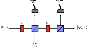
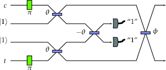
Figure 9: The NS gate by Rudolph and Pan. Based on a vacuum detection of the first output port, and a single vertically polarised photon on the second output port, the interferometer applies an NS gate to the input state. The success probability is also $(3-\sqrt{2})/7$, which is close to the optimal value of 1/4.

Figure 10: The Knill CZ gate based on two ancilla photons and two detected photons. The beam splitter angles are $\theta=54.74$ and $\phi=17.63$, such that the transmission amplitudes are given by $\cos\theta$ and $\cos\phi$, respectively.

Sometimes it might be sufficient to apply destructive two-photon gates. For example, a Bell measurement in teleportation does not need to be non-destructive in order to sucessfully teleport a photon. In this case, we can increase the probability of success of the gate considerably. A CNOT gate that needs post-selection to make sure there is one polarised photon in each output mode was proposed by Ralph et al.  (2002a). It makes use only of beam splitters with reflection coefficient of 1/3, and polarising beam splitters. The success probability is 1/9. An identical gate was proposed independently by Hofmann and Takeuchi (2002). It was also shown that the success probability of an array of $n$ CZ gates of this type can be made to operate with a probability of $p=(1/3)^{n+1}$, rather than $p=(1/9)^{n}$ Ralph (2004).

II.2 Parity gates and entangled ancillæ

A special optical gate that will become important in section III is the so-called parity check. It consists of a single polarizing beam splitter, followed by photon detection in the complementary basis of one output mode. If the input modes are denoted by $a$ and $b$, and the output modes are $c$ and $d$, then the Bogoliubov transformation is given by Eq. (10). For two input qubits in the computational basis $\{|H\rangle,|V\rangle\}$ this gate induces the following transformation:

$$|H,H\rangle_{ab} \rightarrow |H,H\rangle_{cd},$$ (44)

$$|H,V\rangle_{ab} \rightarrow |HV,0\rangle_{cd},$$ (45)

$$|V,H\rangle_{ab} \rightarrow |0,HV\rangle_{cd},$$ (46)

$$|V,V\rangle_{ab} \rightarrow |V,V\rangle_{cd},$$ (47)

where $|HV,0\rangle_{cd}$ denotes a vertically and horizontally polarised photon in mode $c$, and nothing in mode $d$. Making a projective measurement in mode $c$ onto the complementary basis $(|H\rangle\pm|V\rangle)/\sqrt{2}$ then yields a parity check: If we detect a single photon in mode $c$, we know that the input qubits had the same logical value. This value is transmitted into the output qubit in mode $d$ (up to a $\sigma_{z}$ transformation depending on the measurement result). On the other hand, if we detect zero or two photons in mode $c$, the input qubits were not identical. In this case, the state of the output mode is no longer in the single-qubit subspace.

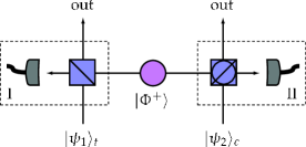
Figure 11: The CNOT gate by Pittman et al. (2001). The two boxes I and II are parity gates in two complementary bases, where the detector measures in a complementary basis with respect to the polarising beam splitter. The gate makes use of a maximally entangled ancillary state $|\Phi^{+}\rangle$, which boosts the success probability up to one quarter. The target $|\psi_{1}\rangle_{t}$ and control $|\psi_{2}\rangle_{c}$ input states will evolve into an entangled output state conditioned on the required detector signature.

This gate was used by Cerf, Adami, and Kwiat to construct small optical quantum circuits (1998). As we have seen in section I.4, however, their approach is not scalable since $n$-qubit circuits involve $2^{n}$ distinct paths. When two parity gates in complementary bases are combined with a maximally entangled ancilla state $|\Phi^{+}\rangle=(|H,H\rangle+|V,V\rangle)/\sqrt{2}$, a CNOT gate with success probability 1/4 is obtained Pittmann et al. (2001); Koashi et al. (2001). The setup is shown in Fig. 11.

For a detailed analysis of several probabilistic gates, see Lund and Ralph (2002), Gilchrist et al. (2003), and Lund et al. (2003). General two-qubit gates based on Mach-Zehnder interferometry were proposed by Englert et al. (2001). For a general discussion of entanglement in quantum information processing see Paris et al. (2003).

All the gates that we have discussed so far are probabilistic, and indeed all two-qubit gates based on projective measurements must be probabilistic. However, it is in principle still possible that feed-forward protocols can increase the probability to unity. As mentioned before, Knill (2003) demonstrated that this is not the case, and that instead the highest possible success probability for the NS gate (using feed-forward) is one half. He did not show that this bound is tight. Indeed, numerical evidence strongly suggests an upper bound of one third for infinite feed-forward without entangled ancillæ Scheel et al. (2005). This indicates that the benefit of feed-forward might not outweigh its cost.

II.3 Experimental demonstrations of gates

A number of experimental groups have already demonstrated all-optical probabilistic quantum gates. Early experiments involved a parity check of two polarisation qubits on a polarising beam splitter Pittman et al. 2002b , and a two-photon conditional phase switch Resch et al. (2002). A destructive CNOT gate was demonstrated by Franson et al. (2003) and O’Brien et al.  (2003). In this section we will describe the experimental demonstration of three CNOT gates.

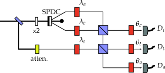
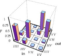
Figure 12: Schematic diagram of the experimental setup of the three-photon CNOT gate of Pittman et al. (2003). The gate starts by preparing the qubits with polarization rotations $\lambda_{i}$, followed by mixing the ancilla and control qubits on a polarising beam splitter. The ancilla qubit then is mixing with the target qubit on the second polarising beam splitter. The gate is implemented upon a three-fold detector coincidence in the control, target, and ancilla modes. The polarization rotations $\theta_{i}$ are used to select different polarization bases.

Figure 13: Experimental demonstration of the CNOT gate by Pittman et al. (2003). The figure shows the probability of 3-fold coincidences as a function of the output qubit analysers for all four computational basis states $HH,HV,VH,VV$ in the input registers. The error in the gate is approximately 21%.

First, we consider the three-photon CNOT gate performed by Pittman, Fitch, Jacobs, and Franson (2003). The gate is shown in Fig. 13 and consists of three polarisation-encoded single photon qubits and two polarising beam splitters. Two of the polarisation qubits represent the control and target qubits and are initially in an arbitrary two qubit state $|\psi\rangle_{\rm in}=\alpha_{1}|HH\rangle_{ct}+\alpha_{2}|HV\rangle_{ct}+\alpha_{3}|VH\rangle_{ct}+\alpha_{4}|VV\rangle_{ct}$. The third photon is used as an ancilla qubit and is initially prepared in the state $(|H\rangle+|V\rangle)/\sqrt{2}$. In the Pittman et al. experiment the control qubit and the ancillary qubit are created using pulsed parametric down conversion. The target qubit is generated by an attenuated laser pulse where the pulse is branched off the pump laser. The pulse is converted by a frequency doubler to generate entangled photon pairs at the same frequency as the photon constituting the target qubit. The CNOT gate is then implemented as follows: The action of the polarising beam splitters on the control, target and ancilla qubits transforms them according to

$$|\psi\rangle_{\rm out}\propto|H\rangle_{a}U_{\rm C}|\psi\rangle_{\rm in}+|V\rangle_{a}\widetilde{U}_{\rm C}|\psi\rangle_{\rm in}+\sqrt{6}|\xi\rangle_{act},$$ (48)

where $U_{\rm C}$ is the CNOT operator between the control and target modes $c$ and $t$ and $\widetilde{U}_{\rm C}=(\mbox{\small 1}\!\!\mbox{1}\otimes\sigma_{x})\,U_{\rm C}\,(\mbox{\small 1}\!\!\mbox{1}\otimes\sigma_{x})$. The state $|\xi\rangle_{act}$ represent terms with zero, two, or three photons present in the modes $a$, $c$, and $t$. Depending on the polarisation of the measured ancillary photon in mode $a$ (and one photon in the control and target modes) a CNOT gate up to a local transformation is applied to the control and target qubits. For a horizontally measured $|H\rangle_{a}$ photon the CNOT gate is exactly implemented, while for a vertically measured $|V\rangle_{a}$ photon the control and target qubits undergo a CNOT gate up to a bit flip on the target qubit. In Fig. 13 the truth table is shown as a function of the output qubit analysers for all four computational basis states $HH,HV,VH,VV$ in the input. The success probability for this gate is $p=1/4$ with an error of approximately 21%.

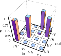
Figure 14: Schematic diagram of the CNOT gate demonstrated by O’Brien et al. (2003). (a) Concept of the two-qubit gate: The beam splitter coefficients are $\theta_{1}=\pi/4$ and $\theta_{2}=\arccos(1/\sqrt{3})$. (b) Translation circuit for converting polarisation and dual rail qubits. (c) Schematic of the experimental setup. Simultaneous detection of a single photon at each of the detectors heralds the successful operation of the gate.

Figure 15: Experimental demonstration of the CNOT gate by O’Brien et al. (2003) in the logical qubit basis. The data is obtained by full state tomography of the output states.

The second experiment we consider is the CNOT gate by O’Brien, Pryde, White, Ralph, and Branning, depicted in Fig. 15 O’Brien et al. (2003), which is an implementation of the gate proposed by Ralph et al. (2002a). This is a post-selected two-photon gate where the two polarised qubits are created in a parametric down conversion event. The polarisation qubits can be converted into which-path qubits via a translation stage depicted in Fig. (15b). Both the control and target qubits can be prepared in an arbitrary pure superposition of the computational basis states.

The gate is most easily understood in terms of dual spatial rails, Fig. (15a). The two spatial modes that support the target qubit are mixed on a 50:50 beam splitter ($\theta_{1}=\pi/4$). One of these output modes is mixed with a spatial mode of the control qubit on a beam splitter with $\cos\theta_{2}=1/\sqrt{3}$ (that is, a beam splitter with a reflectivity of 33$\frac{1}{3}$%). To balance the probability distribution of the CNOT gate, two “dump ports” consisting of another beam splitter with $\cos\theta_{2}=1/\sqrt{3}$ are introduced in one of the control and target modes. The gate works as follows: If the control qubit is in the state where the photon occupies the top mode $c_{0}$ there is no interaction between the control and the target qubit. On the other hand, when the control photon is in the lower mode, the control and target photons interfere non-classically at the central beam splitter with $\cos\theta_{2}=1/\sqrt{3}$. This two-photon quantum interference causes a $\pi$ phase shift in the upper arm of the target interferometer $t_{0}$, and as a result, the target photon is switched from one output mode to the other. In other words, the target state experiences a bit flip. The control qubit remains unaffected, hence the interpretation of this experiment as a CNOT gate. We do not always observe a single photon in each of the control and target outputs. However, when a control and target photon are detected we know that the CNOT operation has been correctly realized. The success probability of such an event is $1/9$. The detection of the control and target qubits could in principle be achieved by a quantum non-demolition measurement (see section IV.1) and would not destroy the information encoded on the qubits. Experimentally, beam displacers are used to spatially separate the polarisation modes, and waveplates are used for the beam-mixing.

In Fig. 15, we show the truth table for the CNOT operation in the coincidence basis. The fidelity of the gate is approximately 84% with conditional fringe visibilities exceeding 90% in non-orthogonal bases. This indicates that entanglement has been generated in the experiment: The gate can create entangled output states from separable input states.

The last experiment we consider in some detail is the realization of an optical CNOT by Gasparoni, Pan, Walther, Rudolph, and Zeilinger (2004). The experiment is based on the four-photon logic gate by Pittman et al. (2001) depicted in Fig. 11.

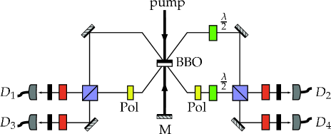
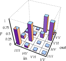
Figure 16: Schematic diagram of the four-photon CNOT gate by Gasparoni et al. (2004). A parametric down conversion source is used to create the control and target input qubits in the spatial modes $a_{1}$ and $a_{2}$, as well as a maximally entangled ancilla pair in the spatial modes $a_{3}$ and $a_{4}$. Polarising filters (Pol) can be used to destroy the initial entanglement in $a_{1}$ and $a_{2}$ if necessary.

Figure 17: Experimental demonstration of the CNOT gate by Gasparoni et al. (2004). Four-fold coincidences for all combinations of inputs and outputs are shown.

The Gasparoni et al. experiment employs a type-II parametric down conversion source operated in a “double-pass” arrangement. The down-conversion process naturally produces close to maximally entangled photon pairs. This means that, depending on the input state for the control and target qubits, we may have to destroy or decrease any initial polarisation entanglement. This is achieved by letting the photons pass through appropriate polarisation filters. After this, any two-qubit input state can be prepared. The gate depicted in Fig. 17 works as follows: The control qubit and one half of the Bell state are sent into a polarising beam splitter, while the target qubit with the second half of the Bell state are sent through a second polarising beam splitter. The detection of the ancilla photons heralds the operation of the CNOT gate (up to a known bit or sign flip on the control and/or target qubit). The probability of success of this gate is $1/4$. Due to a lack of detectors that can resolve the difference between one and two photons and the rather low source and detector efficiencies, four-fold coincidence detection was employed to confirm the presence of photons in the output control and target ports. In principle, this post-selection can be circumvented by using deterministic Bell pair sources and detectors that differentiate between one and two incoming photons.

The CNOT truth table for this experiment, based on four-fold coincidences, is shown in Fig. 17. This shows the operation of the CNOT gate. In addition, Gasparoni et al. showed that an equal superposition of $H$ and $V$ for the control qubit and $H$ for the target qubit generated the maximally entangled state $|HH\rangle+|VV\rangle$ with a fidelity of $81\%$. This clearly shows that the gate is creating entanglement.

As experiments become more sophisticated, more demonstrations of optical gates are reported. We cannot describe all of them here, but other recent experiments include the nonlinear sign shift Sanaka et al. (2004), a non-destructive CNOT Zhao et al. (2005), another CNOT gate Fiorentino and Wong (2004), and three-qubit optical quantum circuits Takeuchi 2000b ; Takeuchi (2001). Four-qubit cluster states, which we will encounter later in this review, were demonstrated by Walther et al.  (2005).

II.4 Characterisation of linear optics gates

In section II.3, we showed the experimentally realised CNOT truth table for three different experimentally realised gates. However, the construction of the truth table is in itself not sufficient to show that a CNOT operation has been performed. It is essential to show the quantum coherence of the gate. One of the simplest ways to show coherence is to apply the gate to an initial separate state and show that the gate creates an entangled state (or vice versa). For instance, the operation of a CNOT gate on the initial state $(|H\rangle_{c}-|V\rangle_{c})|V\rangle_{t}$ creates the maximally entangled singlet state $|H\rangle_{c}|V\rangle_{t}-|V\rangle_{c}|H\rangle_{t}$. This is sufficient to show the coherence properties of the gate. However, showing such coherences does not fully characterise the gate. To this end, we can perform state tomography. We show an example of this for the CNOT gate demonstrated by O’Brien et al. (2003) in Fig. 18. The reconstructed density matrix clearly indicates that a high-fidelity singlet state has been produced.

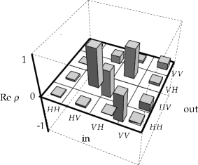
Figure 18: Plot of the real part of the density matrix reconstructed from quantum process tomography for the input state $(|H\rangle_{c}-|V\rangle_{c})|V\rangle_{t}$. This shows the highly entangled singlet state of the form $|H\rangle_{c}|V\rangle_{t}-|V\rangle_{c}|H\rangle_{t}$

To fully understand the operation of a gate we need to create a complete map $\hat{\mathcal{E}}$ of all the input states to the output states.

$$\hat{\mathcal{E}}(\rho)=\sum_{m,n=0}^{d-1}\chi_{mn}{\hat{A}}_{m}\rho{\hat{A}}^{\dagger}_{n},$$ (49)

This map represents the process acting on an arbitrary input state $\rho$, where the operators ${\hat{A}_{m}}$ form a basis for the operators acting on $\rho$. The matrix $\chi$ describes completely the process $\hat{\mathcal{E}}$. Once this map has been constructed, we know everything about the process, including the purity of the operation and the entangling power of the gate. This information can then be used to fine-tune the gate operation. Experimentally, the map is obtained by performing quantum process tomography Chuang and Nielsen (1997); Poyatos et al. (2001). A set of measurements is made on the output of the $n$-qubit quantum gate, given a complete set of input states. The input states and measurement projectors each form a basis for the set of $n$-qubit density matrices. For the two-qubit CNOT gate ($d=16$), we require 256 different settings of input states and measurement projectors.

In Fig. 19, we reproduce the reconstructed process matrix $\chi$ for the CNOT gate performed by O’Brien et al. (2003). The ideal CNOT can be written as a coherent sum: ${\hat{U}}_{\rm CNOT}=\tfrac{1}{2}(\mbox{\small 1}\!\!\mbox{1}\otimes\mbox{\small 1}\!\!\mbox{1}+\mbox{\small 1}\!\!\mbox{1}\otimes X+Z\otimes\mbox{\small 1}\!\!\mbox{1}-Z\otimes X)$ of tensor products of Pauli operators $\{\mbox{\small 1}\!\!\mbox{1},X,Y,Z\}$ acting on control and target qubits respectively. The process matrix shows the populations/coherences between the basis operators making up the gate. The process fidelity for this gate exceeds 90% (see also O’Brien et al. 2004). For a general review of quantum state tomography with an emphasis on quantum information processing, see Lvovsky and Raymer (2005).

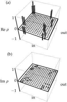
Figure 19: Plot of the real (a) and imaginary (b) parts of the reconstructed process matrix of the CNOT gate by O’Brien et al. (2003). The ideal CNOT can be written as a coherent sum: ${\hat{U}}_{\rm CNOT}=\tfrac{1}{2}(\mbox{\small 1}\!\!\mbox{1}\otimes\mbox{\small 1}\!\!\mbox{1}+\mbox{\small 1}\!\!\mbox{1}\otimes X+Z\otimes\mbox{\small 1}\!\!\mbox{1}-Z\otimes X);$ of the tensor products of Pauli operators $\{\mbox{\small 1}\!\!\mbox{1},X,Y,Z\}$ acting on control and target qubits respectively.

II.5 General probabilistic nonlinear gates

The two-qubit gates described above are special cases of $N$ ports acting on a set of input states, followed by a projective measurement. For quantum computing applications, however, we usually want the resulting nonlinear transformation $\mathsf{M}$ to be unitary. This is because non-unitary operations will reveal information about the qubits in the projective measurement, and hence corrupts the computation. We can derive a simple criterion that the $N$ ports and the projective measurements must satisfy Lapaire et al. (2003).

Suppose the qubits undergoing $\mathsf{M}$ span a Hilbert space ${\mathcal{H}}_{Q}$, and the auxiliary qubits span ${\mathcal{H}}_{A}$. Furthermore, let $U$ be the unitary transformation of the $N$ port in Eq. (14) and $P_{k}$ the projector on the auxiliary states denoting the measurement outcome labelled by $k$. $P_{k}$ must be a projector on the Hilbert space with dimension $\dim{\mathcal{H}}_{A}$ for $\mathsf{M}$ to be unitary. Given an arbitrary input state $\rho$ of the qubits and a state $\sigma$ of the auxiliary systems, the output state can be written as

$$\rho_{\mathrm{out}}^{(k)}=\frac{\mathrm{Tr}_{A}\left[U(\rho\otimes\sigma)U^{\dagger}P_{k}\right]}{\mathrm{Tr}_{QA}\left[U(\rho\otimes\sigma)U^{\dagger}P_{k}\right]}\;.$$ (50)

When we define $d(\rho)\equiv\mathrm{Tr}_{QA}\left[U(\rho\otimes\sigma)U^{\dagger}P_{k}\right]$, we find that $\mathsf{M}$ is unitary if and only if $d(\rho)$ is independent of $\rho$. We can then construct a test operator $\hat{T}=\mathrm{Tr}_{A}\left(\sigma U^{\dagger}P_{k}U\right)$. The induced operation on the qubits in ${\mathcal{H}}_{Q}$ is then unitary if and only if $\hat{T}$ is proportional to the identity, or

$$\hat{T}=\mathrm{Tr}_{A}\left(\sigma U^{\dagger}P_{k}U\right)\propto\mbox{\small 1}\!\!\mbox{1}~{}\Leftrightarrow~{}d(\rho)=d\;.$$ (51)

Given the auxiliary input state $\sigma$, the $N$ port transformation $U$ and the projective measurement $P_{k}$, it is straightforward to check whether this condition holds. The success probability of the gate is given by $d$.

In Eq. (50), the projective measurement was in fact a projection operator $(P_{k}^{2}=P_{k})$. However, in general, we might want to include generalised measurements, commonly known as Positive Operator-Valued Measures, or POVMs. These are particularly useful when we need to distinguish between nonorthogonal states, and they can be implemented with $N$ ports as well Myers and Brandt (1997). Other optical realizations of non-unitary transformations were studied by Bergou et al. (2000).

The inability to perform a deterministic two-qubit gate such as the CNOT with linear optics alone is intimately related to the impossibility of complete Bell measurements with linear optics Lütkenhaus et al. (1999); Vaidman and Yoran (1999); Calsamiglia (2002). Since quantum computing can be cast into the shape of single-qubit operations and two-qubit projections Nielsen (2003); Leung (2004), we can approach the problem of making nonlinear gates via complete discrimination of multi-qubit bases.

Van Loock and Lütkenhaus gave straightforward criteria for the implementation of complete projective measurements with linear optics van Loock and Lütkenhaus (2004). Suppose the basis states we want to identify without ambiguity are given by $\{|s_{k}\rangle\}$, and the auxiliary state is given by $|\psi_{\mathrm{aux}}\rangle$. Applying the unitary $N$ port transformation yields the state $|\chi_{k}\rangle$. If the outgoing optical modes are denoted by $a_{j}$, with corresponding annihilation operators $\hat{a}_{j}$, then the set of conditions that have to be fulfilled for $\{|\chi_{k}\rangle\}$ to be completely distinguishable are

$$\langle\chi_{k}|\hat{a}_{j}^{\dagger}\hat{a}_{j}|\chi_{l}\rangle=0 \forall j$$ (52)

$$\langle\chi_{k}|\hat{a}_{j}^{\dagger}\hat{a}_{j}\hat{a}_{j^{\prime}}^{\dagger}\hat{a}_{j^{\prime}}|\chi_{l}\rangle=0 \forall j,j^{\prime}$$ (53)

$$\langle\chi_{k}|\hat{a}_{j}^{\dagger}\hat{a}_{j}\hat{a}_{j^{\prime}}^{\dagger}\hat{a}_{j^{\prime}}\hat{a}_{j^{\prime\prime}}^{\dagger}\hat{a}_{j^{\prime\prime}}|\chi_{l}\rangle=0 \forall j,j^{\prime},j^{\prime\prime}$$ (54)

$$\vdots\qquad \vdots$$ (55)

Furthermore, when we keep the specific optical implementation in mind, we can use intuitive physical principles such as photon number conservation and group-theoretical techniques such as the decomposition of $U(N)$ into smaller groups. This gives us an insight into how the auxiliary states and the photon detection affects the (undetected) signal state Scheel et al. (2003).

So far we have generally focused on the means necessary to perform single-qubit rotations and CNOT gates. It is well known that such gates are sufficient for universal computation. However, it is not necessary to restrict ourselves to such a limited set of operations. Instead, it is possible to extend our operations to general circuits that can be constructed from linear elements, single photon sources, and detectors. This is analogous to the shift in classical computing from a RISC (Reduced Instruction Set Computer) architecture to the CISC (Complex Instruction Set Computer) architecture. The RISC-based architecture in quantum computing terms could be thought of as a device built only from the minimum set of gates, while a CISC-based machine would be built from a much larger set; a natural set of gates allowed by the fundamental resources. The quantum SWAP operation illustrates this point. From fundamental gates, three CNOTs are required to build such an operation. However, from fundamental optical resources only two beam splitters and a phase shifter are necessary. Scheel et al. (2003) focused their attention primarily on one-mode and two-mode situations, though the approach is easily extended to multi-mode situations. They differentiated between operations that are easy and that are potentially difficult. For example, operations that cause a change in the Fock layers (for instance the Hadamard operator) are generally difficult but not impossible.

II.6 Scalable optical circuits and quantum teleportation

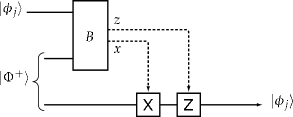
Figure 20: The CZ applied to two qubits inside a quantum circuit. If it fails, then the two qubit states are lost.

Figure 21: The teleportation circuit. The state $|\phi_{j}\rangle$ is teleported via an entangled quantum channel $|\Phi^{+}\rangle$ and a Bell measurement $B$. The binary variables $x$ and $z$ parameterise the outcome of the Bell measurement and determine which Pauli operator is applied to the output mode.

When the gates in a computational circuit succeed only with a certain probability $p$, then the entire calculation that uses $N$ such gates succeeds with probability $p^{N}$. For large $N$ and small $p$, this probability is minuscule. As a consequence, we have to repeat the calculation on the order of $p^{-N}$ times, or run $p^{-N}$ such systems in parallel. Either way, the resources (time or circuits) scale exponentially with the number of gates. Any advantage that quantum algorithms might have over classical protocols is thus squandered on retrials or on the amount of hardware we need. In order to do useful quantum computing with probabilistic gates, we have to take the probabilistic elements out of the running calculation.

In 1999, Gottesman and Chuang proposed a trick that removes the probabilistic gate from the quantum circuit, and places it in the resources that can be prepared off-line Gottesman and Chuang (1999). It is commonly referred to as the teleportation trick, since it “teleports the gate into the quantum circuit.”

Suppose we need to apply a probabilistic CZ gate to two qubits with quantum states $|\phi_{1}\rangle$ and $|\phi_{2}\rangle$ respectively. If we apply the gate directly to the qubits, we are very likely to destroy the qubits (see Fig. 21). However, suppose that we teleport both qubits from their initial mode to a different mode. For one qubit, this is shown in Fig. 21. Here, $x$ and $z$ are binary variables, denoting the outcome of the Bell measurement, which determine the unitary transformation that we need to apply to the output mode. If $x=1$, we need to apply the $\sigma_{x}$ Pauli operator (denoted by $X$), and if $z=1$, we need to apply $\sigma_{z}$ (denoted by $Z$). If $x,z=0$ we do not apply the respective operator. For teleportation to work, we also need the entangled resource $|\Phi^{+}\rangle$, which can be prepared off-line. If we have a suitable storage device, we do not have to make $|\Phi^{+}\rangle$ on demand: we can create it with a probabilistic protocol using several trials, and store the output of a successful event in the storage device.

When we apply the probabilistic CZ gate to the output of the two teleportation circuits, we effectively have again the situation depicted in Fig. 21, except that now our circuit is much more complicated. Since the CZ gate is part of the Clifford group, we can commute it through the Pauli operators $X$ and $Z$ at the cost of more Pauli operators. This is good news, because that means we can move the CZ gate from the right to the left, and only incur the optically available single-qubit Pauli gates. Instead of preparing two entangled quantum channels $|\Phi^{+}\rangle$, we now have to prepare the resource $\mbox{\small 1}\!\!\mbox{1}\otimes U_{\rm CZ}\otimes\mbox{\small 1}\!\!\mbox{1}|\Phi^{+}\rangle\otimes|\Phi^{+}\rangle$ (see Fig. 22). Again, with a suitable storage device, this can be done off-line with a probabilistic protocol. There are now no longer any probabilistic elements in the computational circuit.

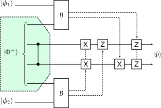
Figure 22: The CZ gate using teleportation: here, $|\psi\rangle=U_{\rm CZ}|\phi_{1}\phi_{2}\rangle$. By commuting the CZ gate through the Pauli gates from the computational circuit to the teleportation resources, we have taken the probabilistic part off-line. We can prepare the teleportation channel (the shaded area, including the CZ) in many trials, without disrupting the quantum computation.

II.7 The Knill-Laflamme-Milburn protocol

Unfortunately, there is a problem with the teleportation trick when applied to linear optics: In our qubit representation the Bell measurement (which is essential to quantum teleportation) is not complete, and works at best only half of the time Lütkenhaus et al. (1999); Vaidman and Yoran (1999). It seems that we are back where we started. This is one of the problems of linear optical quantum computing that was solved by Knill, Laflamme, and Milburn (2001).

In the KLM scheme, the qubits are chosen from the dual-rail representation. However, in the KLM protocol the teleportation trick applies to the single-rail state $\alpha|0\rangle+\beta|1\rangle$, where $|0\rangle$ and $|1\rangle$ denote the vacuum and the single-photon Fock state respectively, and $\alpha$ and $\beta$ are complex coefficients (this is because the CZ gate involves only one optical mode of each qubit). Linearity of quantum mechanics ensures that if we can teleport this state, we can also teleport any coherent or incoherent superposition of such a state.

Choose the quantum channel to be the $2n$-mode state

$$|t_{n}\rangle=\frac{1}{\sqrt{n+1}}\sum_{j=0}^{n}|1\rangle^{j}|0\rangle^{n-j}\;|0\rangle^{j}|1\rangle^{n-j},$$ (56)

where $|k\rangle^{j}\equiv|k\rangle_{1}\otimes\ldots\otimes|k\rangle_{j}$. We can then teleport the state $\alpha|0\rangle+\beta|1\rangle$ by applying an $n+1$-point discrete quantum Fourier transform (QFT) to the input mode and the first $n$ modes of $|t_{n}\rangle$, and count the number of photons $m$ in the output mode. The input state will then be teleported to mode $n+m$ of the quantum channel (see Fig. 23).

Figure 23: Near-deterministic teleportation according to Knill, Laflamme and Milburn. The input state $|\phi\rangle=\alpha|0\rangle+\beta|1\rangle$ is teleported to the $m^{\rm th}$ outgoing mode, where $m$ is the number of detected photons in the measurement of the $(n+1)$-point quantum Fourier transform. Note that $|\psi\rangle$ is a single-rail state; $0$ and $1$ denote photon numbers here.

The discrete quantum Fourier transform $F_{n}$ can be written in matrix notation as:

$$(F_{n})_{jk}=\frac{1}{\sqrt{n}}\exp\left[2\pi i\;\frac{(j-1)(k-1)}{n}\right].$$ (57)

It erases all path information of the incoming modes, and can be interpreted as the $n$-mode generalisation of the 50:50 beam splitter. To see how this functions as a teleportation protocol, it is easiest to consider an example.

Suppose, we choose $n=5$, such that the state $|t_{n}\rangle$ describes ten optical modes, and assume further that we count two photons ($m=2$). This setup is given in Fig. 24. The two rows of zeros and ones denote two terms in the superposition $|t_{5}\rangle$. The five numbers on the left are the negative of the five numbers on the right (from which we will choose the outgoing qubit mode). It is then clear from this diagram that when we find two photons, there are only two ways this could come about: either the input mode did not have a photon (associated with amplitude $\alpha$), in which case the two photons originated from $|t_{5}\rangle$, or the input mode did have a photon, in which case the state $|t_{5}\rangle$ provided the second photon. However, by construction of $|t_{5}\rangle$, the second mode of the five remaining modes must have the same number of photons as the input mode. And because we erased the which-path information of the measured photons using the $F_{6}$ transformation, the two possibilities are added coherently. This means that we teleported the input mode to mode $5+2=7$. In order to keep the amplitudes of the output state equal to those of the input state, the relative amplitudes of the terms in $|t_{n}\rangle$ must be equal.

Sometimes, this procedure fails, however. When we count either zero or $n+1$ photons in the output of the QFT, we collapsed the input state onto zero or one photons respectively. In those cases we know that the teleportation failed. The success rate of this protocol is $n/(n+1)$ (where we used that $|\alpha|^{2}+|\beta|^{2}=1$). We can make the success probability of this protocol as large as we like by increasing the number of modes $n$. The success probability for teleporting a two-qubit gate is then the square of this probability, $n^{2}/(n+1)^{2}$, because we need to teleport two qubits successfully. The quantum teleportation of a superposition state of a single photon with the vacuum was realized by Lombardi et al. (2002) using spontaneous parametric down-conversion.

Now that we have a (near-) deterministic teleportation protocol, we have to apply the probabilistic gates to the auxiliary states $|t_{n}\rangle$. For the CZ gate, we need the auxiliary state

$$|cz_{n}\rangle = \frac{1}{n+1}\sum_{i,j=0}^{n}(-1)^{(n-i)(n-j)}|1\rangle^{i}|0\rangle^{n-i}$$ (59)

$$\;\times|0\rangle^{i}|1\rangle^{n-i}\;|1\rangle^{j}|0\rangle^{n-j}\;|0\rangle^{j}|1\rangle^{n-j}\;.$$

The cost of creating this state is quite high. In the next section we will see how the addition of error correcting codes can alleviate this resource count somewhat.

Figure 24: The 5-photon ancillary scheme for near-deterministic teleportation.

At this point, we should resolve a paradox: Earlier results have shown that it is impossible to perform a deterministic Bell measurement with linear optics. However, teleportation relies critically on a Bell measurement of some sort, and we have just shown that we can perform near-deterministic teleportation with only linear optics and photon counting. The resolution in the paradox lies in the fact that the impossibility proofs are concerned with exact deterministic Bell measurements. The KLM variant of the Bell measurement always has an arbitrarily small error probability $\epsilon$. We can achieve scalable quantum computing by making $\epsilon$ smaller than the fault-tolerant threshold.

One way to boost the probability of success of the teleportation protocol is to minimise the amplitudes of the $j=0$ and $j=n$ terms in the superposition $|t_{n}\rangle$ of Eq. (56). At the cost of changing the relative amplitudes (and therefore introducing a small error in the teleported output state), the success probability of teleporting a single qubit can then be boosted to $1-1/n^{2}$ Franson et al. (2002). The downside of this proposal is that the errors become less well-behaved: Instead of perfect teleportation of the state $\alpha|0\rangle+\beta|1\rangle$ with an occasional $\sigma_{z}$ measurement of the qubit, the Franson variation will yield an output state $c_{j}\alpha|0\rangle+c_{j-1}\beta|1\rangle$, where $j$ is known and the $c_{j}$ are the amplitudes of the modified $|t_{n}\rangle$. There is no simple two-mode unitary operator that transforms this output state into the original input state without knowledge about $\alpha$ and $\beta$. This makes error correction much harder.

Another variation on the KLM scheme due to Spedalieri et al. (2005) redefines the teleported qubit $\alpha|0\rangle+\beta|1\rangle$ and Eq. (56). The vacuum state is replaced with a single horizontally polarised photon, $|0\rangle\rightarrow|H\rangle$, and the one-photon state is replaced with a vertically polarised photon, $|1\rangle\rightarrow|V\rangle$. There are now $2n$ rather than $n$ photons in the state $|t_{n}\rangle$. The teleportation procedure remains the same, except that we now count the total number of vertically polarised photons. The advantage of this approach is that we know that we should detect exactly $n$ photons. If we detect $m\neq n$ photons, we know that something went wrong, and this therefore provides us with a level of error detection (see also section V).

Of course, having a near-deterministic two-qubit gate is all very well, but if we want to do arbitrarily long quantum computations, the success probability of the gates must be close to one. Instead of making larger teleportation networks, it might be more cost effective or easier to use a form of error correction to make the gates deterministic. This is the subject of the next section.

II.8 Error correction of the probabilistic gates

As we saw in the previous section the probability of success of teleportation gates can be increased arbitrarily by preparing larger entangled states. However the asymptotic behaviour to unit probability is quite slow as a function of $n$. A more efficient procedure is to encode against gate failure. This is possible because of the well-defined failure mode of the teleporters. We noted in the previous section that the teleporters fail if zero or $n+1$ photons are detected because we can then infer the logical state of the input qubit. In other words the failure mode of the teleporters is to measure the logical value of the input qubit. If we can encode against accidental measurements of this type then our qubit will be able to survive gate failures and the probability of eventually succeeding in applying the gate will be increased.

KLM introduced the following logical encoding over two polarisation qubits:

$$|0\rangle_{L} = |HH\rangle+|VV\rangle$$

$$|1\rangle_{L} = |HV\rangle+|VH\rangle$$ (60)

This is referred to as parity encoding as the logical zero state is an equal superposition of the even parity states and the logical one state is an equal superposition of the odd parity states. Consider an arbitrary logical qubit: $\alpha|0\rangle_{L}+\beta|1\rangle_{L}$. Suppose a measurement is made on one of the physical qubits returning the result $H$. The effect on the logical qubit is the projection:

$$\alpha|0\rangle_{L}+\beta|1\rangle_{L}\to\alpha|H\rangle+\beta|V\rangle$$ (61)

That is, the qubit is not lost, the encoding is just reduced from parity to polarisation. Similarly if the measurement result is $V$ we have:

$$\alpha|0\rangle_{L}+\beta|1\rangle_{L}\to\alpha|V\rangle+\beta|H\rangle$$ (62)

Again the superposition is preserved, but this time a bit-flip occurs. However, the bit-flip is heralded by the measurement result and can therefore be corrected.

Suppose we wish to teleport the logical value of a parity qubit with the $t_{1}$ teleporter. We attempt to teleport one of the polarisation qubits. If we succeed we measure the value of the remaining polarisation qubit and apply any necessary correction to the teleported qubit. If we fail we can use the result of the teleporter failure (did we find zero photons or two photons?) to correct the remaining polarisation qubit. We are then able to try again. In this way the probability of success of teleportation is increased from $1/2$ to $3/4$. At this point we have lost our encoding in the process of teleporting. However, this can be fixed by introducing the following entanglement resource:

$$|H\rangle|0\rangle_{L}+|V\rangle|1\rangle_{L}$$ (63)

If teleportation is successful, the output state remains encoded. The main observation is that the resources required to construct the entangled state of Eq. (63) are much less than those required to construct $|t_{3}\rangle$. As a result, error encoding turns out to be a more efficient way to scale up teleportation and hence gate success.

Parity encoding of an arbitrary polarisation qubit can be achieved by performing a CNOT gate between the arbitrary qubit and an ancilla qubit prepared in the diagonal state, where the arbitrary qubit is the target and the ancilla qubit is the control. This operation has been demonstrated experimentally O’Brien et al. (2005). In this experiment the projections given by Eqs. (61) and (62) were confirmed up to fidelities of 96%. In a subsequent experiment by Pittman et al., the parity encoding was prepared in a somewhat different manner and, in order to correct the bit-flip errors, a feed-forward mechanism was implemented Pittman et al. (2005).

To boost the probability of success further, we need to increase the size of the code. The approach adopted by Knill, Laflamme and Milburn (2001) was to concatenate the code. At the first level of concatenation the parity code states become:

$$|0\rangle_{L}^{(4)} = |00\rangle_{L}+|11\rangle_{L}$$

$$|1\rangle_{L}^{(4)} = |01\rangle_{L}+|10\rangle_{L}$$ (64)

This is now a four-photon encoded state. At the second level of concatenation we would obtain an eight-photon state etc. At each higher level of concatenation, corresponding encoded teleportation circuits can be constructed that operate with higher and higher probabilities of success.

If we are to use encoded qubits we must consider a universal set of gates on the logical qubits. An arbitrary rotation about the $x$-axis, defined by the operation $X_{\theta}=\cos{(\theta/2)}I-i\sin{(\theta/2)}X$, is implemented on a logical qubit by simply implementing it on one of the constituent polarisation qubits. However, to achieve arbitrary single qubit rotations we also require a $\pi/2$ rotation about the $z$-axis, i.e. $Z_{\pi/2}=1/\sqrt{2}(I-iZ)$. This can be implemented on the logical qubit by applying $Z_{\pi/2}$ to each constituent qubit and then applying a CZ gate between the constituent qubits. The CZ gate is of course non-deterministic and so the $Z_{\pi/2}$ gate becomes non-deterministic for the logical qubit. Thus both the $Z_{\pi/2}$ and the logical CZ gate must be implemented with the teleportation gates in order to form a universal gate set for the logical qubits. In Ref. Knill et al. (2000) it is reported that the probability of successfully implementing a $Z_{\pi/2}$ gate on a parity qubit in this way is $P_{Z}=1-F_{Z}$ where

$$F_{Z}=\frac{f^{2}(2-f)}{1-f(1-f)}$$ (65)

and $f$ is the probability of failure of the teleporters acting on the constituent polarisation qubits. One can obtain the probability of success after concatenation iteratively. For example the probability of success after one concatenation is $P_{Z1}=1-F_{Z1}$ where $F_{Z1}=F_{Z}^{2}(2-F_{Z})/(1-F_{Z}(1-F_{Z}))$. The probability of success for a CZ gate between two logical qubits is $P_{CZ}=(1-F_{Z})^{2}$. Notice that, for this construction, an overall improvement in gate success is not achieved unless $f<1/2$. Using these results one finds that first level concatenation and $t_{3}$ ($f=1/4$) teleporters are required to achieve a CZ gate with better than 95% probability of success. It can be estimated that of order $10^{4}$ operations would be required in order to implement such a gate Hayes et al. (2004).

So the physical resources for the original KLM protocol, albeit scalable, are daunting. For linear optical quantum computing to become a viable technology, we need more efficient quantum gates. This is the subject of the next section.

III Improvements on the KLM protocol

We have seen that the KLM protocol explicitly tells us how to build scalable quantum computers with single-photon sources, linear optics, and photon counting. However, showing scalability and providing a practical architecture are two different things. The overhead cost of a two-qubit gate in the KLM proposal, albeit scalable, is prohibitively large.

If linear optical quantum computing is to become a practical technology, we need less resource-intensive protocols. Consequently, there have been a number of proposals that improve the scalability of the KLM scheme. In this section we review these proposals. Several improvements are based on cluster-state techniques Yoran and Reznik (2003); Nielsen (2004); Browne and Rudolph (2005), and recently a circuit-based model of optical quantum computing was proposed that circumvents the need for the very costly KLM-type teleportation Gilchrist et al. (2005). After a brief introduction to cluster state quantum computing, we will describe these different proposals.

Figure 25: A typical cluster state. Every circle represents a logical qubit, and the vertices represent CZ operations. A quantum computation proceeds by performing single-qubit measurements on the left column of qubits, thus removing them from the cluster and teleporting the quantum information through the cluster state. The vertical links induce two-qubit operations.

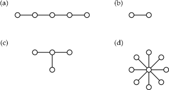
Figure 26: Different cluster and graph states. (a) A linear cluster of five qubits. (b) A cluster representing the Bell states. (c) A four-qubit GHZ state. This state can be obtained by an $X$-measurement of the central qubit in (a). (d) A general GHZ state.

III.1 Cluster states in optical quantum computing

In the traditional circuit-based approach to quantum computing, quantum information is encoded in qubits, which subsequently undergo single- and two-qubit operations. There is, however, an alternative model, called the cluster-state model of quantum computing Raussendorf and Briegel (2001). In this model, the quantum information encoded in a set of qubits is teleported to a new set of qubits via entanglement and single-qubit measurements. It uses a so-called cluster state in which physical qubits are represented by nodes and entanglement between the qubits is represented by connecting lines (see Fig. 25). Suppose that the qubits in the cluster state are arranged in a lattice. The quantum computation then consists of performing single-qubit measurements on a “column” of qubits, the outcomes of which determine the basis for the measurements on the next column. Single qubit gates are implemented by choosing a suitable basis for the single-qubit measurement, while two-qubit gates are induced by local measurements of two qubits exhibiting a vertical link in the cluster state.

Two-dimensional cluster states, i.e., states with vertical as well as horizontal links, are essential for quantum computing, as linear cluster-state computing can be efficiently simulated on classical computers Nielsen (2005). Since single-qubit measurements are relatively easy to perform when the qubits are photons, this approach is potentially suitable for linear optical quantum computing: Given the right cluster state, we need to perform only the photon detection and the feed-forward post-processing. Verstraete and Cirac (2004) demonstrated how the teleportation-based computing scheme of Gottesman and Chuang could be related to clusters. They derived their results for generic implementations and did not address the special demands of optics.

Before we discuss the various proposals for efficient cluster-state generation, we present a few more properties of cluster states. Most importantly, a cluster such as the one depicted in Fig. 25 does not correspond to a unique quantum state: It represents a family of states that are equivalent up to local unitary transformations of the qubits. More precisely, a cluster state $|C\rangle$ is an eigenstate of a set of commuting operators $S_{i}$ called the stabiliser generators Raussendorf et al. (2003):

$$S_{i}|C\rangle=\pm|C\rangle\quad\forall i\;.$$ (66)

Typically, we consider the cluster state that is a +1 eigenstate for all $S_{i}$. Given a graphical representation of a cluster state, we can write down the stabiliser generators by following a simple recipe: Every qubit $i$ (node in the graph) generates an operator $S_{i}$. Suppose that a qubit labelled $q$ is connected to $k$ neighbours labelled $1$ to $k$. The stabiliser generator $S_{q}$ for qubit $q$ is then given by

$$S_{q}=X_{q}\,\overset{k}{\underset{j=1}{\mbox{\Large$\otimes$}}}\,Z_{j}\;,$$ (67)

For example, a (simply connected) linear cluster chain of five qubits labelled $a$, $b$, $c$, $d$, and $e$ (Fig. 26a) is uniquely determined by the following five stabiliser generators: $S_{a}=X_{a}Z_{b}$, $S_{b}=Z_{a}X_{b}Z_{c}$, $S_{c}=Z_{b}X_{c}Z_{d}$, $S_{d}=Z_{c}X_{d}Z_{e}$, $S_{e}=Z_{d}X_{e}$. It is easily verified that these operators commute. Note that this recipe applies to general graph states, where every node (i.e., a qubit) can have an arbitrary number of links with other nodes. The rectangular shaped cluster states are a subset of the set of graph states.

Consider the following important examples of cluster and graph states: The connected two-qubit cluster state is locally equivalent to the Bell states (Fig. 26b), and a linear three-qubit cluster state is locally equivalent to a three-qubit GHZ (Greenberger-Horne-Zeilinger) state. These are states that are locally equivalent to $|0,\ldots,0\rangle+|1,\ldots,1\rangle$. In general, GHZ states can be represented by a star-shaped graph such as shown in Figs. 26c and 26d.

To build the cluster state that is needed for a quantum computation, we can transform one graph state into another using entangling operations, single-qubit operations and single-qubit measurements. A $Z$ measurement removes a qubit from a cluster and severs all the bonds that it had with the cluster Raussendorf et al. (2003); Hein et al. (2004). An $X$ measurement on a qubit in a cluster removes that qubit from the cluster, and it will transfer all the bonds of the original qubit to a neighbour. All the other neighbours become single connected qubits to the neighbour that inherited the bonds Raussendorf et al. (2003); Hein et al. (2004).

There is a well-defined physical recipe for creating cluster or graph states, such as the one shown in Fig. 25. First of all, we prepare all qubits in the state $(|0\rangle+|1\rangle)/\sqrt{2}$. Secondly, we apply a CZ-gate to all qubits that are to be linked with a horizontal or vertical line, the order of which does not matter.

To make a quantum computer using the one-way quantum computer, we need two-dimensional cluster states Nielsen (2005). Computation on linear cluster chains can be simulated efficiently on a classical computer. Furthermore, two-dimensional cluster states can be created with Clifford group gates. The Gottesman-Knill theorem then implies that the single-qubit measurements implementing the quantum computation must include non-Pauli measurements.

It is the entangling operation that is problematic in optics, since a linear optical CZ gate in our qubit representation is inherently probabilistic. There have been, however, several proposals for making cluster or graph states with linear optics and photon detection, and we will discuss them in chronological order.

III.2 The Yoran-Reznik protocol

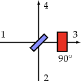
Figure 27: Using the “hyper-entanglement” of the polarisation and which-path observables, a single photon spans a four-dimensional Hilbert space $\{|H,1\rangle,|H,2\rangle,|V,1\rangle,|V,2\rangle\}$. A simple 50:50 beam-splitter and polarisation rotation then furnishes a deterministic transformation from the computational basis to the Bell basis.

The first proposal for linear optical quantum computing along these lines by Yoran and Reznik (2003) is not strictly based on the cluster-state model, but it has many attributes in common. Most notably, it uses “entanglement chains” of photons in order to pass the quantum information through the circuit via teleportation.

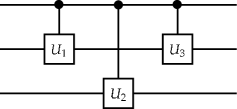
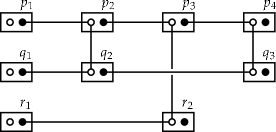
Figure 28: A typical three-qubit quantum computational circuit.

Figure 29: The computational circuit of Fig. 29 in terms of the physical implementation by Yoran and Reznik (2003). This is reminiscent of the cluster-state model of quantum computing. The open and closed dots represent the polarisation and which-path degrees of freedom, respectively.

First of all, for this protocol to work, the nondeterministic nature of optical teleportation must be circumvented. We have already remarked several times that complete (deterministic) Bell measurements cannot be performed in the dual-rail and polarisation qubit representations of linear optical quantum computing. However, in a different representation this is no longer the case. Instead of the traditional dual-rail implementation of qubits, we can encode the information of two qubits in a single photon when we include both the polarisation and the spatial degree of freedom. Consider the device depicted in Fig. 27. A single photon carrying specific polarisation and path information is then transformed as Popescu (1995):

$$|H,1\rangle ~{}\rightarrow~{} \frac{1}{\sqrt{2}}\left(|V,3\rangle+|H,4\rangle\right)$$ (68)

$$|V,1\rangle ~{}\rightarrow~{} \frac{1}{\sqrt{2}}\left(|V,4\rangle-|H,3\rangle\right)$$ (69)

$$|H,2\rangle ~{}\rightarrow~{} \frac{1}{\sqrt{2}}\left(|H,4\rangle-|V,3\rangle\right)$$ (70)

$$|V,2\rangle ~{}\rightarrow~{} \frac{1}{\sqrt{2}}\left(|V,4\rangle+|H,3\rangle\right)\;.$$ (71)

These transformations look tantalisingly similar to the transformation from the computational basis to the Bell basis. However, there is only one photon in this system. The second “qubit” is given by the which-path information of the input modes. By performing a polarisation measurement of the output modes $3$ and $4$, we can project the input modes onto a “Bell state”. This type of entanglement is sometimes called hyper-entanglement, since it involves more than one observable of a single system Kwiat and Weinfurter (1998); Barreiro et al. (2005); Cinelli et al. (2005). A teleportation experiment based on this mechanism was performed by Boschi et al. (1998).

It was shown by Yoran and Reznik how these transformations can be used to cut down on the number of resources: Suppose we want to implement the computational circuit given in Fig. 29. We will then create (highly entangled) chain states of the form

$$(\alpha|H\rangle_{p_{1}}+\beta|V\rangle_{p_{1}})(|1\rangle_{p_{1}}|H\rangle_{p_{2}}+|2\rangle_{p_{1}}|V\rangle_{p_{2}})\times\ldots$$ (72)

$$\times(|2n-1\rangle_{p_{n}}|H\rangle_{p_{n+1}}+|2n\rangle_{p_{n}}|V\rangle_{p_{n+1}})|2n+1\rangle_{p_{n+1}},$$ (73)

where the individual photons are labelled by $p_{j}$. This state has the property that a Bell measurement of the form of Eq. (68) on the first photon $p_{1}$ will teleport the input qubit $\alpha|H\rangle+\beta|V\rangle$ to the next photon $p_{2}$.

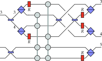
Figure 30: How to add a link to the YR chain. This will create the state given in Eq. (72) with $n+1=5$. The four vertically connected grey circles represent the probabilistic CZ gate. Note that we need two of them.

Let’s assume that we have several of these chains running in parallel, and that furthermore, there are vertical “cross links” of entanglement between different chains, just where we want to apply the two-qubit gates $U_{1}$, $U_{2}$, and $U_{3}$. This situation is sketched in Fig. 29. The translation into optical chain states is given in Fig. 29. The open circles represent polarisation, and the dots represent the path degree of freedom. In Fig. 30, the circuit that adds a link to the chain is shown. The unitary operators $U_{1}$, $U_{2}$, and $U_{3}$ are applied to the polarisation degree of freedom of the photons.

Note that we still need to apply two probabilistic CZ gates in order to add a qubit to a chain. However, whereas the KLM scheme needs the teleportation protocol to succeed with very high probability (scaling as $n^{2}/(n+1)^{2}$) in the protocol proposed by Yoran and Reznik the success probability of creating a link in the chain must be larger than one half. This way, the entanglement chains grow on average. This is a very important observation and plays a key role in the protocols discussed in this section. Similarly, a vertical link between the entanglement chains can be established with a two-qubit unitary operation on the polarisation degree of freedom of both photons (c.f. the vertical lines between the open dots in Fig. 29). If the gate fails, we can grow longer chains and try again until the gate succeeds.

III.3 The Nielsen protocol

A more explicit use of cluster-state quantum computing was made by Nielsen (2004). As Yoran and Reznik, Nielsen recognised that in order to build cluster states, the probability of adding a link to the cluster must be larger than one half, rather than arbitrarily close to one. Otherwise the cluster will shrink on average. The KLM teleportation protocol allows us to apply a two-qubit gate with probability $n^{2}/(n+1)^{2}$, depending on the number $n$ of ancillary photons. Let us denote a CZ gate with this success probability by $CZ_{n^{2}/(n+1)^{2}}$. This gate can be used to add qubits to a cluster chain. When the gate fails, it removes a qubit from the cluster. This means that, instead of using very large $n$ to make the CZ gate near-deterministic, links can be added on average with a modest $CZ_{9/16}$-gate, or $n=3$. This leads to similarly reduced resource requirements as the Yoran-Reznik protocol, while still keeping (in principle) error-free quantum computing. However, there is an extra gain in resources available when we try to add a qubit to a chain Nielsen (2004).

Suppose that we wish to add a single qubit to a cluster chain via the teleportation-based CZ gate. Instead of teleporting the two qubits simultaneously, we first teleport the disconnected qubit, and secondly teleport the qubit at the end of the cluster. We know that a teleportation failure will remove the qubit from the cluster, so we attempt the second teleportation protocol only after the first has succeeded. The first teleportation protocol then becomes part of the off-line resource preparation, and the CZ gate effectively changes from $CZ_{n^{2}/(n+1)^{2}}$ to $CZ_{n/(n+1)}$. The growth requirement of the cluster state then becomes $n/(n+1)>1/2$, or $n=2$, and we make another substantial saving in resources.

Apart from linear cluster states, we also need the ability to make the two-dimensional clusters depicted in Fig. 25. This is equivalent to linking a qubit to two cluster chains, and hence needs two successful CZ gates. Arguing along the same lines as before, it is easily shown that the success probability is 4/9 for this procedure using two ancillæ per teleportation gate. Since this is smaller than one half, this procedure on average removes qubits from the cluster. However, we can first add extra qubits with the previous procedure, such that there is a buffer of qubits in the cluster state. This way, the average shrinkage of the cluster due to vertical links is absorbed by the buffer region.

Finally, Nielsen introduces so-called micro-clusters consisting of multiple qubits connected to the end point of a cluster chain. Such a micro-cluster is depicted in Fig. 26d, where the central qubit is an endpoint of a cluster chain. Having such a fan of qubits at the end of a chain, we can retry the entangling gate as many times as there are “dangling” qubits. This removes the lower limit on the success probability of the CZ gate at the cost of making large GHZ states Nielsen and Dawson (2004). Therefore, any optical two-qubit gate with arbitrary success probability $p$ can be used to make cluster states efficiently.

III.4 The Browne-Rudolph protocol

There is still a cheaper way to grow cluster states. In order for a cluster chain to grow on average without using expensive micro-clusters, the success probability of adding a single qubit to the chain must be larger than one half. However, if we can add small chains of qubits to the cluster, this requirement may be relaxed. Suppose that the success probability of creating a link between two cluster chains is $p$, and that in each successful linking of two chains we lose $d_{s}$ qubits from the chain. This might happen when the entangling operation joining the two clusters involves the detection of qubits in the cluster. Similarly, in an unsuccessful attempt, we may lose $d_{f}$ qubits from the existing cluster chain (we do not count the loss of qubits in the small chain that is to be added). If our existing cluster chain has length $N$, and the chain we wish to add has length $m$, then we can formulate the following growth requirement Barrett and Kok (2005); Browne and Rudolph (2005):

$$p(N+m-d_{s})+(1-p)(N-d_{f})>N$$ (75)

$$\Leftrightarrow m>\frac{p\,d_{s}+(1-p)d_{f}}{p}\;.$$ (76)

Given a specific strategy $(d_{s},d_{f})$ and success probability $p$, we need to create chains of length $m$ off-line in order to make large cluster chains efficiently. Note that, again, there is no lower limit to the success probability $p$ of the entangling operation in principle. This allows us to choose the optical gates with the most desirable physical properties (other than high success probability), and it means that we do not have to use the expensive and error-prone $CZ_{n/(n+1)}$ gates.

Indeed, Browne and Rudolph introduced a protocol for generating cluster states using the probabilistic parity gates of section II.2 Browne and Rudolph (2005); Cerf et al. (1998); Pittmann et al. (2001). The notable advantage of this gate is that it is relatively easy to implement in practice Pittman et al. 2002b , and that it can be made robust against common experimental errors. Initially these gates were called parity gates, but following Browne and Rudolph, we call these the type-I and type-II fusion gates (see Fig. 31).

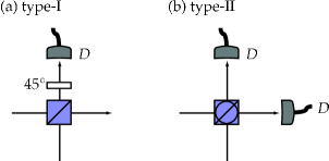
Figure 31: Two types of fusion operators. (a) the type-I fusion operator employs a polarisation beam splitter (PBS1) followed by the detection $D$ of a single output mode in the 45^∘ rotated polarisation basis. This operation determines the parity of the input mode with probability 1/2. (b) the type-II fusion operator uses a diagonal polarisation beam splitter (PBS2), detects both output modes, and projects the input state onto a maximally entangled Bell state with probability 1/2.

Let us first consider the operation of the type-I fusion gate in Fig. 31a. Given the detection of one and only one photon with polarisation $H$ or $V$ in the detector $D$, the gate induces the following projection on the input state:

$$\text{``H''}: \frac{1}{\sqrt{2}}\left(|H\rangle\langle H,H|-|V\rangle\langle V,V|\right)$$ (77)

$$\text{``V''}: \frac{1}{\sqrt{2}}\left(|H\rangle\langle H,H|+|V\rangle\langle V,V|\right).$$ (78)

It is easily verified that the probability of success for this gate is $p=1/2$. When the type-I fusion gate is applied to two photons belonging to two different cluster states containing $n_{1}$ and $n_{2}$ photons, respectively, a successful operation will generate a cluster chain of $n_{1}+n_{2}-1$ photons. However, when the gate fails, it effectively performs a $\sigma_{z}$ measurement on both photonic qubits, and the two cluster states both lose the qubit that was detected. The type-I fusion gate is therefore a $(1,1)$-strategy, i.e., $d_{s}=d_{f}=1$ (recall that we count only the loss of qubits on one cluster to determine $d_{f}$). The ideal growth requirement is $m>1/p=2$.

Browne and Rudolph also introduced the type-II fusion operator (see Fig. 31b). This operation involves the photon detection of both output modes of a polarisation beam splitter, and a successful event is heralded by a detector coincidence (i.e., one photon with a specific polarisation in each detector). When successful, this gate projects the two incoming qubits onto one of two polarisation Bell states, depending on the detection outcome:

$$\text{``H,V'' or ``V,H''}: \frac{1}{\sqrt{2}}\left(|H,H\rangle+|V,V\rangle\right)$$ (79)

$$\text{``H,H'' or ``V,V''}: \frac{1}{\sqrt{2}}\left(|H,V\rangle+|V,H\rangle\right).$$ (80)

The success probability of this gate is $p=1/2$, and it is a $(2,1)$-strategy (i.e., $d_{s}=2$ and $d_{f}=1$). The ideal growth requirement is thus $m>(1+p)/p=3$. The type-II fusion gate is essentially a version of the incomplete optical Bell measurement Braunstein and Mann (1996); Weinfurter (1994).

Note that in order to grow long chains, we must be able to create chains of three qubits. Given a plentiful supply of Bell pairs as our fundamental resource, we can make three-qubit chains only with the type-I fusion gate, since the type-II gate necessarily destroys two qubits. This also indicates a significant difference between this protocol and the previous ones: Using only single-photon sources, the fusion gates alone cannot create cluster states. We can, however, use any method to create the necessary Bell pairs (such as the CZ gate in section II.1), as they constitute an off-line resource.

Upon successful operation, both the type-I and the type-II fusion gates project two qubits that are part of a cluster onto a polarisation Bell state. When we apply a Hadamard operation to one of the qubits adjacent to the detected qubit(s), the result will again be a cluster state. However, upon failure the characteristics of the fusion gates are quite different from each other. When the type-I gate fails, it performs a $Z$ measurement on the input qubits. When the type-II gate fails, it performs an $X$ measurement on the input qubits. Recall that there is a fundamental difference between a $Z$ and an $X$ measurement on qubits in cluster states: A $Z$ measurement will break all bonds with the qubits neighbours and removes it from the cluster. An $X$ measurement will also remove the qubit from the cluster, but it will join its neighbours into a redundantly encoded qubit. In terms of the graphs, this corresponds to a qubit with dangling bonds called leaves or cherries (see also Fig. 26c).

When the measured qubits are both end points of cluster states (i.e., they have only one link to the rest of the cluster), failing type-I and type-II fusion gates have similar effects on the cluster states: They remove the qubits from the cluster. However, when the fusion gates are applied to two qubits inside a cluster (i.e., the qubits have two or more links to other qubits in the cluster), then the failure modes of the two fusion gates differ dramatically: In particular when we apply the fusion gate to a qubit in a chain, a failed type-I gate will break the chain, while a failed type-II gate will only shorten the chain and create one redundantly encoded qubit next to the measured qubit. Since it is costly to re-attach a broken chain, it is best to avoid the type-I gate for this purpose. The redundancy induced by a failed type-II fusion gate is closely related to the error correction model in section V. We will explore this behaviour further in the next section.

Again, we need at least two-dimensional cluster states in order to achieve the level of quantum computing that cannot be simulated efficiently on a classical computer. Using the failure behaviour of the type-II fusion gate, we can construct an efficient way of creating the vertical links between linear cluster chains. We attempt a type-II fusion between two qubits that are part of different chains. If the gate succeeds, we have created a vertical link on the neighbouring qubits. If the gate fails, one neighbouring qubit to each detected qubit becomes redundantly encoded. The type-I fusion can now be attempted once more on the redundantly encoded qubits. If the gate succeeds, we established a vertical link. If the gate fails, we end up with two disconnected chains that are both two qubits shorter. Given sufficiently long linear cluster chains, we can repeat this protocol until we have succeeded in creating a vertical link. A proof-of-principle experiment demonstrating optical cluster-state quantum computing with four photons was performed in Vienna Walther et al. (2005).

III.5 Circuit-based optical quantum computing revisited

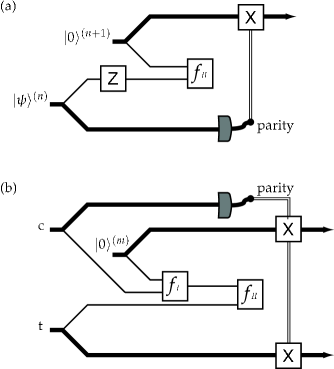
Figure 32: The two probabilistic gates that complete a universal set. (a) the $Z_{\pi/2}$ gate uses a deterministic single-photon rotation and a single type-II fusion gate. (b) the CNOT gate uses one type-I and one type-II fusion gate. Both gates also need a parity measurement, which is implemented by $\sigma_{z}$ measurements on the individual physical qubits.

After all this, one might conclude that the cluster-state approach to linear optical quantum information processing has completely replaced the circuit-based model. However, such a conclusion would be premature. In fact, in a slightly altered form, the redundancy that we encountered in the Browne-Rudolph protocol can be used to make a scalable circuit-based optical quantum computer Hayes et al. (2004); Gilchrist et al. (2005). We will now show how this is done.

We can encode a logical qubit in $n$ physical qubits using the parity encoding we encountered earlier in section II.8:

$$|0\rangle^{(n)} \equiv \frac{1}{\sqrt{2}}\left(|+\rangle^{\otimes n}+|-\rangle^{\otimes n}\right)$$ (81)

$$|1\rangle^{(n)} \equiv \frac{1}{\sqrt{2}}\left(|+\rangle^{\otimes n}-|-\rangle^{\otimes n}\right),$$ (82)

where $|\pm\rangle=(|H\rangle\pm|V\rangle)/\sqrt{2}$. The superscript $(n)$ denotes the level of encoding. This encoding has the attractive property that a computational-basis measurement of one of the physical qubits comprising the logical qubit $|\psi\rangle^{(n)}$ will yield $|\psi\rangle^{(n-1)}$, up to a local unitary on a single (arbitrary) physical qubit. In other words, no quantum information has been lost Gilchrist et al. (2005).

One way to generate this encoding is to use the type-II fusion operator without the two polarisation rotations (half-wave plates) in the input ports of the polarising beam splitter. This yields

$$f_{II}|\psi\rangle^{(n)}|0\rangle^{(m)}\rightarrow\left\{\begin{array}[]{cl}|\psi\rangle^{(n+m-2)}&\mbox{(success)}\\ |\psi\rangle^{(n-1)}|0\rangle^{(m-1)}&\mbox{(failure),}\end{array}\right.$$ (83)

with $|\psi\rangle^{(n)}\equiv\alpha|0\rangle^{(n)}+\beta|1\rangle^{(n)}$. From this, we can immediately deduce that, given a success probability $p$, the growth requirement for the redundancy encoding is $m>(1+p)/p$. This is exactly the same scaling behaviour as the Browne-Rudolph protocol when clusters are grown with the type-II fusion gate.

In order to build circuits that are universal for quantum computing, we need a set of single-qubit operations, and at least one two-qubit entangling gate at the level of the parity encoded quits. As we have seen in section II.8, we can perform the operations $X_{\theta}$ and $Z$ deterministically: The operator $X_{\theta}\equiv\cos(\theta/2)\mbox{\small 1}\!\!\mbox{1}+i\sin(\theta/2)\sigma_{x}$ can be implemented by applying this single-qubit operator to only one physical qubit of the encoding. The $Z$ gate for an encoded qubit corresponds to a $\sigma_{z}$ operation on all the physical qubits.

To complete the universal set of gates, we also need the single-qubit gate $Z_{\pi/2}$ and the CNOT. These gates cannot be implemented deterministically on parity-encoded qubits. In Fig. 32 we show how to implement these gates using the fusion operators. The thickness of the lines denotes the level of encoding. In addition to the fusion operators, we need to perform a parity measurement on one of the qubits by doing $\sigma_{z}$ measurements on all the physical qubits in a circuit line. Since this measurement is performed on a subset of the physical qubits comprising a logical qubit, no quantum information is lost in this procedure. It should also be noted that we attempt the probabilistic fusion gates before the destructive parity measurement, so that in the case of a failed fusion operation, we still have sufficient redundancy to try the fusion again. It has been estimated that universal gate operations can be implemented with $>99\%$ probability of success with about $10^{2}$ operations Gilchrist et al. (2005).

This circuit-based protocol for linear optical quantum computation has many features in common with the Browne-Rudolph protocol. Although the cluster-state model is conceptually quite different from the circuit-based model, they have similar resource requirements. Another point that the reader might be wondering about, is whether these schemes are tolerant to photon loss and other practical noise. The errors that we discussed so far originate from the probabilistic nature of linear optical photon manipulation, but can we also correct errors that arise from, e.g., detection inefficiencies? We will discuss the realistic errors of linear optical component in the next section, and the possible fault tolerance of LOQC in the presence of these errors in section V.

IV Realistic optical components and their errors

In order to build a real quantum computer based on linear optics, single-photon sources, and photon detection, our design must be able to deal with errors: The unavoidable errors in practical implementations should not erase the quantum information that is present in the computation. We have already seen that the teleportation trick in the KLM scheme employs error correction to turn the non-deterministic gates into near-deterministic gates. However, this assumes that the photon sources, the mode matching of the optical circuits, and the photon counting are all perfect. In the real world, this is far from true.

What are the types of errors that can occur in the different stages of the quantum computation? We can group them according to the optical components: detection errors, source errors, and circuit errors Takeuchi 2000a . In this section we will address these errors. In addition, we will address an assumption that has received little attention thus far: the need for quantum memories.

IV.1 Photon detectors

In linear quantum optics, the main method for gaining information about the quantum states is via photon detection. Theoretically, we can make a distinction between at least two types of detectors: ones that tell us exactly how many photons there are in an input state, and ones that give a binary output “nothing” or “many”. There are many more possible distinctions between detectors, but these two are the most important. The first type is called a number-resolving detector or a detector with single-photon resolution, while the second type is often called a bucket or vacuum detector. The original KLM proposal relies critically on the availability of number-resolving detectors. On the other hand, typical photon detectors in LOQC experiments are bucket detectors. In recent years there has been a great effort to bridge the gap between the requirements of LOQC and the available photon detectors, leading to the development of number-resolving detectors and LOQC protocols that rely less on high photon-number counting. In this section, we state the common errors that arise in realistic photon detection and review some of the progress in the development of number-resolving detectors.

Real photon detectors of any kind give rise to two different types of errors:

1. The detector counts fewer photons than were actually present in the input state. This is commonly known as photon loss;

2. the detector counts more photons than were actually present in the input state. These are commonly known as dark counts.

Observe that it is problematic to talk about the number of photons “that were actually present” in the input state: When the input state is a superposition of different photon number states, the photon number in the state prior to detection is ill-defined. However, we can give a general meaning to the concepts of photon loss and dark counts for arbitrary input states when we define the loss or dark counts as a property of the detector (i.e., independent of the input state). The detector efficiency $\eta\in[0,1]$ can be defined operationally as the probability that a single photon input state will result in a detector count, while the dark counts can be defined as the probability that a vacuum input state will result in a detector count. Subsequently, these definitions can be modified to take into account non-poissonian errors.

Whereas perfect number-resolving detectors can be modelled using the projection operators onto the Fock states $|n\rangle\langle n|$, realistic detectors give rise to Positive Operator Valued Measures, or POVMs. A standard photon loss model is to have a perfect detector be preceded by a beam splitter with transmission coefficient $\eta$ and reflection coefficient $1-\eta$. The reflected mode is considered lost (mathematically, this mode is traced over), so only a fraction $\eta$ of the input reaches the detector. In this model, every incoming photon has the same probability of being lost, leading to Poissonian statistics. The POVM for a number-resolving photon detector corresponding to this model is Scully and Lamb (1969)

$$\hat{E}_{n}=\sum_{k=n}^{\infty}\left({k}\atop{n}\right)\eta^{n}(1-\eta)^{k-n}\;|k\rangle\langle k|\;.$$ (84)

Using the same loss model, the POVM describing the effect of a bucket detector is Kok and Braunstein 2000b

$$\hat{E}_{0} = \sum_{n=0}^{\infty}\;(1-\eta)^{n}\;|n\rangle\langle n|$$ (85)

$$\hat{E}_{1} = \sum_{n=0}^{\infty}\;[1-(1-\eta)^{n}]\;|n\rangle\langle n|\;,$$ (86)

where 1 and 0 denote a detector click and no detector click, respectively. For an analysis including dark counts, see Lee et al.  (2004a).

Currently, the most common detectors in experiments on LOQC are Avalanche Photo-Diodes (APDs). When a photon hits the active semi-conductor region of an APD, it will induce the emission of an electron into the conductance band. This electron is subsequently accelerated in an electric potential, causing an avalanche of secondary electrons. The resulting current tells us that a photon was detected. The avalanche must be stopped by reversing the potential, which leads to a dead time of a few nanoseconds in the detector. Any subsequent photon in the input mode can therefore not be detected, and this means that we have a bucket detector. A typical (unfiltered) detector efficiency for such a detector is 85% at a wavelength of 660 nm. Dark counts can be made as low as $6\cdot 10^{3}$ Hz at room temperature and around $25~{}$Hz at cryogenic temperatures.

Several attempts have been made to create a number resolving detector using only bucket detectors and linear optics, but no amount of linear optics and bucket detection can lead to perfect, albeit inefficient, single-photon resolution Kok (2003). On the other hand, we can create approximate number-resolving detectors using only bucket detectors via detector cascading. In this setup, the incoming optical mode is distributed equally over $N$ output modes, followed by bucket detection. When the number of modes in the cascade is large compared to the average photon number in the input state, and the detector efficiencies of the bucket detectors are relatively high, then good fidelities for the photon number measurement can be obtained Kok and Braunstein (2001); Rohde (2005). Detector cascading in the time-domain using increasingly long fibre delays is called time multiplexing Fitch et al. (2003); Achilles et al. (2003); Banaszek and Walmsley (2003). However, the fibre length (and hence the detection time) must increase exponentially for this technique to work. An alternative way to create number-resolving detectors is to use photon-number assisted homodyne detection Nemoto and Braunstein (2002); Branczyk et al. (2003). When an (imperfect) quantum copier is available, extra information can be extracted from the qubits (Deuar and Munro, 2000a, 2000b).

Fully-fledged number-resolving photon detectors are also being developed, such as the Visible Light Photon Counter (VLPC) Takeuchi et al. (1999); Kim et al. (1999). An excellent recent introduction to this technology is given by Waks et al. (2003). The VLPCs operate at a temperature of a few Kelvin in order to minimise dark counts. They consist of an active area that is divided into many separate active regions. When a photon triggers such a region, it is detected while leaving the other regions fully operational. Once a region has detected a photon, it experiences a dead time in which no photon detection can take place. Multiple photon detections in different regions then generate a current that is proportional to the number of photons. The VLPC is thus effectively a large detector cascade ($N\approx 10^{4}$) with high detection efficiency ($\approx 88\%$ at 694 nm). The dark count rate of $2\cdot 10^{4}$ Hz is about an order of magnitude higher than the dark count rate for off-the-shelf APDs.

An alternative technique uses a superconducting transition-edge sensor that acts as a calorimeter. It measures the rise in temperature of an absorber, which is quickly heated by incoming photons in the visible light and near infra-red Rosenberg et al. (2005). This device operates at temperatures well below 100 mK, and has a measured detection efficiency greater than $88\%$. The dark counts are negligible, but the repetition rate is rather slow (of order 10 kHz) due to the cooling mechanism after a photon has been detected. In addition to these experimental schemes, there are theoretical proposals for number-resolving detectors involving atomic vapours James and Kwiat (2002), electromagnetically induced transparency Imamoǧlu (2002), and resonant nonlinear optics Johnsson and Fleischhauer (2003).

Finally, we briefly mention quantum non-demolition (QND) measurements. In the photon detectors that we described so far, the state of the electromagnetic field is invariably destroyed by the detector. However, in a QND measurement there is a freely propagating field mode after the measurement. In particular, the outcome of the QND measurement faithfully represents the state of the field after detection Grangier et al. (1998). Several schemes for single-photon QND measurements have been proposed, either with linear optics Howell and Yeazell 2000a ; Kok et al. (2002), optical quantum relays Jacobs et al. (2002), or other implementations Brune et al. (1990, 1992); Roch et al. (1997); Munro et al. (2005). The experimental demonstration of a single-photon QND was reported by Nogues et al. (1999) using a cavity QED system, and a linear-optical QND measurement was performed by Pryde et al.  (2004). However, this last experiment has led to a controversy about the nature of the fidelity measure that was used (see Kok and Munro, 2005, and Pryde et al. 2005).

So far, we have considered only photon-number detection. However, in many implementations of LOQC the qubit is encoded in a single polarised photon. A qubit detector must therefore extract the polarization of the photon, which may have had unwanted interactions with the environment. A change in the polarization of the photon will then induce an error in the computational circuit.

One mechanism that leads to errors in the polarization is inherent in any photon detector, and deserves a special mention here. In the Coulomb gauge, the polarization is perpendicular to the direction of propagation, and the plane of detection must therefore be perpendicular to the Poynting vector $\vec{k}$. A complication arises when we consider beams that are not perfectly collimated. We can write the $\vec{k}$-vector of the beam as

$$\vec{k}(\theta,\phi)=(\sin\theta\cos\phi,\sin\theta\sin\phi,\cos\theta).$$ (87)

A realistic, reasonably well-collimated beam will have a narrow distribution of $\theta$ and $\phi$ around $\theta_{0}$ and $\phi_{0}$. If we model the active area of a detector as a flat surface perpendicular to $\vec{k}(\theta_{0},\phi_{0})$, some modes in the beam will hit the detector at an angle. Fixing the gauge of the field in the detection plane then causes a mixing of left- and right-handed polarization. This introduces a detection error that is fundamental, since the uncertainty principle prevents the transverse momentum in a beam from being exactly zero Peres and Terno (2002). At first sight this effect might seem negligible, but later we will see that concatenation of error correcting codes will amplify small errors. It is therefore important to identify all possible sources of errors.

IV.2 Photon sources

The LOQC protocols described in this review all make critical use of perfect single-photon sources. In this section we wish to make more precise what is meant by a single-photon source. We have thus far considered interferometric properties of monochromatic plane waves with exactly one field excitation. Such states, while a useful heuristic, are not physical. Our first objective is to give a general description of a single-photon state followed by a description of current experimental realisations.

The notion of a single photon conjures up an image of a single particle-like object localised in space and time. However it was conclusively demonstrated long ago by Newton and Wigner (1949), and also Wightman (1962), that a single photon cannot be localised in the same sense that a single massive particle can be localised. Here we are only concerned with temporal localisation, which is ultimately due to the fact that the energy spectrum of the field is bounded from below. In this section we take a simpler operational view. A photon refers to a single detection event in a counting time window $T$. A single photon source leads to a periodic sequence of single detection events with one and only one, photon detected in each counting window. Further refinement of this definition, via the output counting statistics of interferometers, is needed to specify the kind of single-photon sources necessary for LOQC.

Consider a one-dimensional cavity of length $L$. The allowed wave vectors for plane wave modes form a denumerable set given by $k_{n}=n\pi/L$, with corresponding frequencies $\omega_{n}=ck_{n}$. If we measure time in units of $\pi L/c$, the allowed frequencies may simply be denoted by an integer $\omega_{n}=n\in\mathbb{N}$. Similarly if we measure length in units of $\pi/L$, the allowed wave vectors are also integers. We are primarily interested in multi mode fields with an optical carrier frequency, $\Omega\gg 1$. We define the positive-frequency field component as,

$$\hat{a}(t)=\sum_{n=1}^{\infty}\hat{a}_{n}e^{-int}.$$ (88)

The bosonic annihilation and creation operators are given by Eq. (2). From this point on we assume the detector is located at $x=0$ and thus evaluate all fields at the spatial origin. Following the standard theory of photo-detection, the probability per unit time for detecting a single photon is given by

$$p_{1}(t)=\eta n(t),$$ (89)

where

$$n(t)=\langle\hat{a}^{\dagger}(t)\hat{a}(t)\rangle,$$ (90)

and the parameter $\eta$ characterises the detector.

A single-photon state may be defined as

$$|1;f\rangle=\sum_{m=1}^{\infty}f_{m}\hat{a}_{m}^{\dagger}|0\rangle,$$ (91)

where $|0\rangle=\prod_{m}|0\rangle_{m}$ is the multi-mode global vacuum state, and we require that the single-photon amplitude $f_{m}$ satisfies

$$\sum_{m=0}^{\infty}|f_{m}|^{2}=1.$$ (92)

The counting probability is then determined by

$$n(t)=\left|\sum_{k=1}^{\infty}f_{k}e^{-ikt}\right|^{2}.$$ (93)

This function is clearly periodic with a period $2\pi$. As the spectrum is bounded from below by $n=1$, it is not possible to choose the amplitudes $f_{n}$ so that the functions $n(t)$ have arbitrarily narrow support on $t\in[0,2\pi)$.

As an example we take

$$f^{N}_{m}=\frac{1}{\sqrt{1-(1-\mu)^{N}}}{N\choose m}^{1/2}\mu^{m/2}(1-\mu)^{(N-m)/2},$$ (94)

where we have introduced a cut-off frequency, $N$, making infinite sums finite, and $0\leq\mu\leq 0.5$. For $N\gg 1$ the normalisation is very close to unity, so we will drop it in the following. The dominant frequency in this distribution is $\Omega=\mu N$, which we call the carrier frequency. In this case

$$n(t)=\left|\sum_{k=1}^{N}e^{-ikt}{N\choose k}^{1/2}\mu^{k/2}(1-\mu)^{(N-k)/2}\right|^{2}.$$ (95)

This function is shown in Fig. 33 for various values of $\mu$. The probability per unit time is thus a periodic function of time, with period $2\pi$ and pulse width determined by $\mu$ when $N$ is fixed. If we fix the carrier frequency $\Omega=\mu N$ and let $N$ become large we must let $\mu$ become small. In the limit $N\rightarrow\infty,\ \mu\rightarrow 0$ with $\Omega$ fixed we obtain a Poisson distribution for the single photon amplitude.

Figure 33: The function $n(t)$ in arbitrary units in the domain $-\pi\leq t\leq\pi$ for different values of $\mu$ and $N=100$. (a) $\mu=0.001$; (a) $\mu=0.001$; (b) $\mu=0.01$; (c) $\mu=0.05$; (d) $\mu=0.49$.

A second example is the Lorentzian,

$$f_{n}^{N}=\frac{1}{A}\frac{\sqrt{\mu}}{\mu+in}.$$ (96)

In the limit $N\rightarrow\infty$, the normalisation constant is

$$A=\frac{\pi e^{\mu\pi}}{2\sinh(\mu\pi)}-\frac{1}{2\mu}.$$ (97)

While a field for which exactly one photon is counted in one counting interval, and zero in all others, is no doubt possible, it does not correspond to a more physical situation in which a source is periodically producing pulses with exactly one photons per pulse. To define such a field state we now introduce time-bin operators. For simplicity we assume that only field modes $n\leq N$ are excited and all others are in the vacuum state. It would be more physical to assume only field modes are excited in some band, $\Omega-B\leq n\leq\Omega+B$. Here $\omega$ is the carrier frequency and $2B$ is the bandwidth. However, this adds very little to the discussion.

Define the operators

$$\hat{b}_{\nu}=\frac{1}{\sqrt{N}}\sum_{m=1}^{N}e^{-i\tau m\nu}\hat{a}_{m},$$ (98)

where $\tau=2\pi/N$. This can be inverted to give

$$\hat{a}_{m}=\frac{1}{\sqrt{N}}\sum_{\nu=1}^{N}e^{i\tau m\nu}\hat{b}_{\nu}.$$ (99)

The temporal evolution of the positive frequency components of the field modes then follows from Eq. (88)

$$\hat{a}(t)=\sum_{\mu=1}^{N}g_{\mu}(t)\hat{b}_{\mu},$$ (100)

where

$$g_{\mu}(t)=\frac{1}{\sqrt{N}}\left[1-e^{i(\mu\tau-t)}\right]^{-1}.$$ (101)

The time-bin expansion functions $g_{\mu}(t)$ are a function of $\mu\tau-t$ alone and thus are simple translations of the functions at $t=0$. The form of Eq. (100) is a special case of a more sophisticated way to define time-bin modes. If we were to regard $\hat{a}(t)$ as a classical signal, then the decomposition in Eq. (100) could be generalised as a wavelet transform where the integer $\mu$ labels the translation index for the wavelet functions. In that case the functions $g_{\mu}(t)$ could be made rather less singular. In an experimental context, however, the form of the functions $g_{\mu}(t)$ depends upon the details of the generation process.

The linear relationship between the plane wave modes $a_{m}$ and the time bin modes $b_{\nu}$ is realised by a unitary transformation that does not change particle number, so the vacuum state for the time-bin modes is the same as the vacuum state for the global plane wave modes. We can then define a one-photon time-bin state as

$$\tilde{|1\rangle}_{\mu}=\hat{b}_{\mu}^{\dagger}|0\rangle.$$ (102)

The mean photon number for this state is,

$$n(t)=|g_{\mu}(t)|^{2}.$$ (103)

This function is periodic on $t\in[0,2\pi)$ and corresponds to a pulse localised in time at $t=\mu\tau$. Thus the integer $\mu$ labels the temporal coordinate of the single-photon pulse.

We are now in a position to define an $N$-photon state with one photon per pulse. In addition to the mean photon number, $n(t)$ we can now compute two-time correlation functions such as the second order correlation function, $G^{(2)}(\tau)$ defined by

$$G^{(2)}(T)=\langle\hat{}a^{\dagger}(t)\hat{a}^{\dagger}(t+T)\hat{a}(t+T)\hat{a}(t)\rangle.$$ (104)

The simplest example for $N=2$ is

$$|1_{\mu},1_{\nu}\rangle=\hat{b}_{\mu}^{\dagger}\hat{b}_{\nu}^{\dagger}|0\rangle\ \ \ \ \ \mu\neq\nu.$$ (105)

The corresponding mean photon number is

$$n(t)=|g_{\mu}(t)|^{2}+|g_{\nu}(t)|^{2},$$ (106)

as would be expected. The two-time correlation function is,

$$G^{(2)}(T)=|g_{\mu}(t)g_{\nu}(t+T)+g_{\nu}(t)g_{\mu}(t+T)|^{2}.$$ (107)

Clearly this has a zero at $T=0$ reflecting the fact that the probability to detect a single photon immediately after a single photon detection is zero, as the two pulses are separated in time by $|\mu-\nu|$. This is known as anti-bunching and is the first essential diagnostic for a sequence of single photon pulses with one and only one photon per pulse. When $T=|\mu-\nu|\tau$, however, there is a peak in the two-time correlation function as expected. In Fig. 34 we have reproduced the experimental results for the $G^{(2)}(T)$ from Santori et al. (2002b).

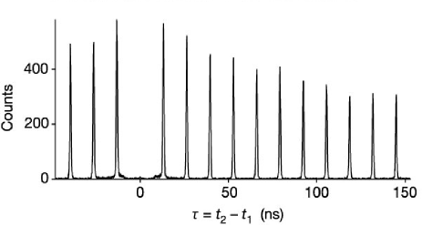
Figure 34: The $G^{(2)}(\tau)$ for the InAs quantum dot single-photon source of Santori et al. (2002b). Note that the variable $T$ in the text is here replaced with $\tau$. Reprinted with permission from Nature Publishing Group.

We now revisit the Hong-Ou-Mandel interferometer introduced in section II.1 with single photon input states. This example has been considered by Rohde and Ralph (2005). We label the two sets of modes by the Latin symbols $a,b$ so, for example, the positive frequency parts of each field are simply $a(t),b(t)$. The coupling between the modes is described by a beam splitter matrix connecting the input and output plane waves

$$\hat{a}_{n}^{out} = \sqrt{\upsilon}\,\hat{a}_{n}+\sqrt{1-\upsilon}\,\hat{b}_{n}$$ (108)

$$\hat{b}_{n}^{out} = \sqrt{\upsilon}\,\hat{b}_{n}-\sqrt{1-\upsilon}\,\hat{a}_{n}$$ (109)

where $0\leq\upsilon\leq 1$. The probability per unit time to find a coincidence detection of a single photon at each output beam is proportional to

$$C=\overline{\langle\hat{a}^{\dagger}(t)\hat{b}^{\dagger}(t)\hat{b}(t)\hat{a}(t)\rangle}.$$ (110)

The over-line represents a time average over a detector response time that is long compared to the period of the field carrier frequencies. In this example, we only need consider the case of one photon in each of the two distinguished modes, so we take the input state to be

$$|1\rangle_{a}\otimes|1\rangle_{b}=\sum_{m,n=1}^{\infty}\alpha_{n}\beta_{m}\hat{a}^{\dagger}_{n}\hat{b}^{\dagger}_{m}|0\rangle,$$ (111)

where $\alpha_{n}$ and $\beta_{n}$ refer to the excitation probability amplitudes for modes $a_{n}$ and $b_{n}$, respectively. This state is transformed by the unitary transformation $U$ to give $|\psi\rangle_{out}=U(|1\rangle_{a}\otimes|1\rangle_{b})$. In the case of a 50:50 beam splitter, for which $\upsilon=0.5$, this is given as ($U|0\rangle=|0\rangle$)

$$|\psi\rangle_{out} = \sum_{n,m=1}^{\infty}\alpha_{n}\beta_{m}\left(Ua_{n}^{\dagger}b_{m}^{\dagger}U^{\dagger}\right)U|0\rangle$$

$$= \frac{1}{2}\sum_{n,m=1}^{\infty}\alpha_{n}\beta_{m}(a_{n}^{\dagger}+b_{n}^{\dagger})(b_{m}^{\dagger}-a_{m}^{\dagger})|0\rangle$$

$$= \frac{1}{2}\sum_{n,m=1}^{\infty}\alpha_{n}\beta_{m}[|1\rangle_{a_{n}}|1\rangle_{b_{m}}-|1\rangle_{a_{n}}|1\rangle_{a_{m}}|0\rangle_{b}$$

$$\mbox{}\ \ \ \ \ \ \ \ \ \ \ \ \ +|1\rangle_{b_{n}}|1\rangle_{b_{m}}|0\rangle_{a}-|1\rangle_{b_{n}}|1\rangle_{a_{m}}].$$

Note that the second and third terms in this sum have no photons in modes $b$ and $a$, respectively. We then have that

$$C=\frac{1}{2}-\frac{1}{2}\sum_{n,m=1}^{\infty}\alpha_{n}\alpha_{m}^{*}\beta_{m}\beta_{n}^{*}.$$ (112)

If the excitation probability amplitudes at each frequency are identical, $\alpha_{n}=\beta_{n}$ this quantity is zero. In other words, only if the two-single photon wave packets are identical do we see a complete cancellation of the coincidence probability. This is the second essential diagnostic for a single-photon source. Of course in practice, complete cancellation is unlikely. The extent to which the coincidence rate approaches zero is a measure of the quality of a single-photon source as far as LOQC is concerned. Whether or not this is the case depends on the nature of the single photon sources. In Fig. 35 we have reproduced the experimental results for the Hong-Ou-Mandel effect, shown with one of the InAs quantum dot single-photon sources of Santori et al. (2002b).

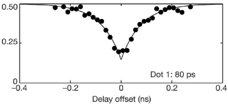
Figure 35: The Hong-Ou-Mandel effect for one of the InAs quantum dot single-photon source of Santori et al. (2002b). Reprinted with permission from Nature Publishing Group.

Broadly speaking, there are currently two main schemes used to realise single photon sources: (I) conditional spontaneous parametric down conversion, and (II) cavity-QED Raman schemes. As discussed by Rohde and Ralph (2005), type (I) corresponds to a Gaussian distribution of $\alpha_{n}$ as a function of $n$ and thus is the continuum analogue of the binomial state defined in Eq. (94). The second scheme, type (II), leads to a temporal pulse structure that is the convolution of the excitation pulse shape and the Lorentzian line shape of a cavity. If the cavity decay time is the longest time in the dynamics, the distribution $\alpha_{n}$ takes the Lorentzian form given in Eq. (96). An early single-photon source based on an optical emitter in a micro-cavity was proposed and demonstrated by De Martini et al. (1996).

Cavity-based single-photon sources are very complicated experiments in their own right, and instead, most single-photon sources used in LOQC experiments are based on Parametric Down-Conversion (PDC). In PDC a short-wavelength pump laser generates photon pairs of longer wavelength in a birefringent crystal. PDC can yield extremely high fidelities ($F>0.99$) because the data is usually obtained via post-selection: we take only those events into account that yield the right number of detector coincidents. In addition, PDC facilitates good mode matching due to energy and momentum conservation in the down-conversion process. The output of a non-collinear type-I PDC can be written as

$$|\Psi_{\rm PDC}\rangle=\sqrt{1-|\lambda|^{2}}\sum_{n=0}^{\infty}\lambda^{n}|n,n\rangle\;,$$ (113)

where $|n\rangle$ is the $n$-photon Fock state, and $\lambda$ is a measure for the amount of down-conversion. The probability for creating $n$ photon pairs is $p(n)=(1-|\lambda|^{2})|\lambda|^{2n}$, which exhibits pair bunching. When $\lambda$ is small, we can make a probabilistic single-photon gun by detecting one of the two modes. However, if we use only bucket detectors without single-photon resolution, then increasing $\lambda$ will also increase the amplitudes for a two-photon pair and ultimately high-photon pairs to the output state. Consequently, the single-photon source will deteriorate badly. A detailed study of the mode structure of the conditional photon pulse has been undertaken by Grice et al.  (2001).

Another consideration regarding parametric down-conversion is that the photons in a pair are typically highly entangled in frequency and momentum. When we use a bucket detector that is sensitive over a broad frequency range to herald a single photon in the freely propagating mode, the lack of frequency information in the detector read-out will cause the single-photon state to be mixed. In principle, this can be remedied by embedding the down-converting material in a micro-cavity such that only certain frequencies are allowed Raymer et al. (2005). The source will then generate photon pairs with frequencies that match the cavity, and a narrow-band bucket detector can herald a pure single-photon state with a small frequency line width.

Alternatively, we can use the following method of making single-photon sources Pittman et al. 2002c ; Migdall et al. (2002): Consider an array of PDCs with one output mode incident on a photon detector, and the other entering the quantum circuit. We fire all PDCs simultaneously. Furthermore, all PDC have small $\lambda$, but if there are approximately $|\lambda|^{-2}$ of them we still create a single photon on average. Given that in current PDC configurations $|\lambda|^{2}\approx 10^{-4}$, this is quite an inefficient process. Nevertheless, since it contributes a fixed overhead per single photon to the computational resources, this technique is strictly speaking scalable. For a detailed description of parametric down-conversion as a photon source see U’Ren et al.  (2003).

To illustrate the experimental constraints on the generation of single-photon states, we now review an example of a cavity-QED Raman scheme implemented by Keller et al.  (2004). Photon anti-bunching from resonance fluorescence was demonstrated long ago. If an atom decays spontaneously from an excited to a ground state, a single photon is emitted and a second photon cannot be emitted until the atom is re-excited. Unfortunately the photon is emitted into a dipole radiation pattern over a complete solid angle. Clearly we need to engineer the electromagnetic environment with mirrors, dielectrics, etc., to ensure a preferred mode for emission. However as pointed out by Kiraz et al.  (2004), this comes at a price. For example, a carefully engineered cavity around a single dipole emitter can change the free field spectral density around the emitter such that a photon is indeed emitted in a preferred direction with an increased rate compared to free space emission.

However, single-photon sources based on spontaneous emission are necessarily compromised by the random nature of spontaneous emission. As demonstrated by Rohde, Ralph, and Nielsen (2005) , single-photon sources that create Gaussian wave packets are much more robust to mode mismatching than sources that create Lorentzian wave packets. Spontaneous emission processes fall in this last category. Clearly, we prefer a stimulated emission process yielding a Gaussian wave packet. To this end, a number of schemes based on stimulated Raman emission into a cavity mode have been proposed Hennrich et al. (2004); Maurer et al. (2004). As an example, we discuss the experiment by Keller et al. (2004) in some detail.

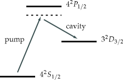
Figure 36: The Raman process in a three-level atom. A classical pump field drives the transition $4^{2}S_{1/2}\rightarrow 4^{2}P_{1/2}$ off-resonantly, thus generating a photon in the cavity mode. The level $4^{2}P_{1/2}$ is adiabatically eliminated and hence never populated.

Consider the three-level atomic system in Fig. 36. The ground state is coupled to the excited state via a two-photon Raman process mediated by a well-detuned third level. In the experiment by Keller et al. (2004), a calcium ion ${}^{40}\mbox{Ca}^{+}$ was trapped in a cavity via an RF ion trap. The cavity field is nearly resonant with the $4^{2}P_{1/2}\rightarrow 3^{2}D_{3/2}$ transition. Initially there is no photon in the cavity. An external laser is directed onto the ion and is nearly resonant with the $4^{2}S_{1/2}\rightarrow 4^{2}P_{1/2}$ transition. When this laser is switched on, the atom can be excited to the $3^{2}D_{3/2}$ level by absorbing one pump photon and emitting one photon in to the cavity. Since this is a stimulated Raman process, the time of emission of the photon into the cavity is completely controlled by the temporal structure of the pump pulse. The photon in the cavity then decays through the end mirror, again as a Poisson process, at a rate given by the cavity decay rate. This can be made very fast.

In principle one can now calculate the probability per unit time to detect a single photon emitted from the cavity. If we assume every photon emitted is detected, this probability is simply $p_{1}(t)=\kappa\langle\hat{a}^{\dagger}(t)\hat{a}(t)\rangle$ where $\kappa$ is the cavity decay rate and $\hat{a},\hat{a}^{\dagger}$ are the annihilation and creation operators for the intra-cavity field and

$$\langle\hat{a}^{\dagger}(t)\hat{a}(t)\rangle=\mbox{\rm tr}[\rho(t)\hat{a}^{\dagger}\hat{a}],$$ (114)

where $\rho(t)$ is the total density operator for ion-plus-cavity-field system. This may be obtained by solving a master equation describing the interaction of the electronic states of the ion and the two fields, one of which is the time-dependent pump. Of course, for a general time-dependent pump pulse-shape this can only be done numerically. Some typical examples are quoted by Keller et al. Indeed by carefully controlling the pump pulse shape considerable control over the temporal structure of the single-photon detection probability may be achieved. In the experiment the length of the pump pulse was controlled to optimise the single-photon output rate. The efficiency of emission was found to be about $8\%$, that is to say, $92\%$ of the pump pulses did not lead to a single-photon detection event. This was in accordance with the theoretical simulations. These photons are probably lost through the sides of the cavity. It is important to note that this kind of loss does not affect the temporal mode structure of the emitted (and detected) photons.

In a similar way we can compute the second-order correlation function via

$$G^{(2)}(T)=\kappa^{2}\mbox{\rm tr}\left[\hat{a}^{\dagger}\hat{a}\,e^{{\cal L}T}(\hat{a}\rho(t)\hat{a}^{\dagger})\right],$$ (115)

where $e^{{\cal L}T}$ is a formal specification of the solution to the master equation for a time $T$ after the “initial” conditional state $a\rho(t)a^{\dagger}$. Once again, due to the non stationary nature of the problem, this must be computed numerically. However, if the pump pulse duration is very short compared to the cavity decay time, and the cavity decay time is the fastest decay constant in the system, the probability amplitude to excite a single photon in a cavity at frequency $\omega$ is very close to Lorentzian. The experiment revealed a clear suppression of the peak at $T=0$ in the normalised correlation function $g^{(2)}(T)$, thus passing the first test of a good single photon source. Unfortunately, a Hong-Ou-Mandel interference experiment was not reported.

For a practical linear-optical quantum computer, however, we need good microscopic single-photon sources that can be produced in large numbers. A recent review on this topic by Lounis and Orrit (2005) identifies six types of microscopic sources: i) Atoms and ions in the gaseous phase; ii) Organic molecules at low temperature and room temperature; iii) Chromophoric systems; iv) Colour centres in diamond, such as nitrogen-vacancy or nickel-nitrogen; v) Semiconductor nano-crystals; and vi) self-assembled quantum dots and other hetero-structures such as micro-pillars and micro-mesa, quantum dots, and electrically driven dots. The typical physical mechanisms that reduce the indistinguishability of the single-photon sources are dephasing of the optical transition, spectral diffusion, and incoherent pumping. An earlier review on this topic is given by Greulich and Thiel (2001). The subject of single-photon sources using quantum dots was reviewed by Santori et al.  (2004).

When single-photon sources are less than ideal, linear optics might be employed in order to improve the output state. For example, if the source succeeds with probability $p$, then the output of the source might be $\rho=p|1\rangle\langle 1|+(1-p)|0\rangle\langle 0|$, where we assumed that the failure output results in a vacuum state. Using multiple copies of $\rho$, linear optics, and ideal photon detection, one may increase the probability up to $p=1/2$, but not higher Berry et al. (2005). A general discussion on improving single-photon sources with linear optical post-processing is given by Berry et al. (2004).

Single-photon sources must not only create clean single-photon states, in the sense described above, but all sources must also generate identical states in order to achieve good visibility in a Hong-Ou-Mandel test. Typical experiments demonstrating single-photon sources create subsequent single-photon states in the same source and employ a delay line to interfere the two photons. This way, two-photon quantum interference effects are demonstrated without having to rely on identical sources Santori et al. 2002b . De Riedmatten et al. demonstrated quantum interference by using identical pulse shapes triggering different photon sources de Riedmatten et al. (2003). In applications other than LOQC, such as cryptography, the requirement of indistinguishable sources may be relaxed. This leads to the concept of the suitability of a source for a particular application Hockney et al. (2003).

A variation on single-photon sources is the entangled-photon source. We define an ideal entangled-photon source as a source that creates a two-photon polarisation Bell state. This is an important resource in both the Browne-Rudolph and the Gilchrist-Hayes-Ralph protocol. It is known that these states cannot be created deterministically from single-photon sources, linear optics and destructive photon detection Kok and Braunstein 2000a . Nevertheless, such states are very desirable, since they would dramatically reduce the cost of linear-optical quantum computing. The same error models for single-photon sources apply to entangled-photon sources. Again, a great variety of proposals for entangled-photon sources exist in the literature, using quantum dots (Benson et al. 2000; Stace et al. 2003) or parametric down-conversion Śliwa and Banaszek (2003). Two-photon states without entanglement have been created experimentally by Moreau et al. (2001), and Santori et al. (2002a), as have entangled photon pairs Yamamoto et al. (2003); Kuzmich et al. (2003).

IV.3 Circuit errors and quantum memories

In addition to detector errors, and errors in the single-photon sources, there is a possibility that the optical circuits themselves acquire errors. Probably the most important circuit error is mode mismatching. It occurs when non-identical wave packets are used in an interferometric setup [e.g., the coefficients $\alpha_{n}$ and $\beta_{n}$ in Eq. (112) are not identical]. There is a plethora of reasons why the coefficients $\alpha_{n}$ and $\beta_{n}$ might not be equal. For example, the optical components might not do exactly what they are supposed to do. More precisely, the interaction Hamiltonian of the components will differ from its specifications. One manifestation of this is that there is a finite accuracy in the parameters in the interaction Hamiltonian of any optical component, leading to changes in phases, beam splitter transmission coefficients, and polarisation rotation angles. In addition, unwanted birefringence in the dielectric media can cause photo-emission and squeezing. Inaccurate Hamiltonian parameters generally reduce the level of mode matching, leading, for example, to a reduced Hong-Ou-Mandel effect and hence inaccurate CZ gates. Indeed, mode matching is likely to be the main circuit error. Most of this effect is due to non-identical photon sources, which we discussed in the previous section. The effect of frequency and temporal mode mismatching was studied by Rohde and Ralph (2005), and by Rohde, Ralph, and Nielsen (2005).

A second error mechanism is that typically, components such as beam splitters, half- and quarter-wave plates, etc. are made of dielectric media that have a (small) absorption amplitude. Scheel (2005) showed that there is a lower bound on the absorption amplitude in physical beam splitters. In addition, imperfect impedance matching of the boundaries will scatter photons back to the source. This amounts to photon loss in the optical circuit. In large circuits, these losses can become substantial.

A third error mechanism is due to classical errors in the feed-forward process. This process consists of the read-out of a photon detector, classical post-processing, and conditional switching of the optical circuit. The detection errors have been discussed in section IV.1 and classical computing is virtually error-free due to robust classical error correction. Optical switches, however, are still quite lossy Thew et al. (2002). In addition, when high-voltage Pockels cells are used, the repetition rate is slow (on the order of 10 kHz). This may become too slow, as photons need to be stored in a quantum memory (e.g., a delay loop), which itself may be lossy and needs feed-forward processing. Feed-forward control for LOQC was demonstrated by Pittman et al.  (2002a) and Giacomini et al. (2002).

An important component of linear optical quantum computing that we have ignored so far is the quantum memory. When the probability of a successful (teleported) gate or addition to a cluster state becomes small, the photons that are part of the circuit must be stored for a considerable time while the off-line preparation of entangled photons is taking place. The use of mere fibre loops then becomes problematic, as these induce photon losses (0.17 dB km^-1 in a standard telecom fibre at 1550 nm). For example, to store a photon for 100 $\mu$s in a fibre has a loss probability of $p\approx 0.54$. At present, all linear optical quantum computer proposals need some kind of quantum memory. This may be in the form of delay lines with error correction, atomic vapours, solid-state implementations, etc.

In general, the effect of a quantum memory error boils down to the inequality of the input state $\rho_{\rm in}$ and the (time-translated) output state $\rho_{\rm out}$. A good figure of merit is the fidelity $F_{qm}$:

$$F_{qm}=\left[\mbox{\rm Tr}\left(\sqrt{\sqrt{\rho_{\rm in}}\,\rho_{\rm out}\,\sqrt{\rho_{\rm in}}}\right)\right]^{2}\;.$$ (116)

The absence of a photon in the output state is an obvious failure mechanism, but other ways the memory can fail include qubit decoherence and mode mismatching of the input/output modes. In this sense, the design specifications of a solid-state based quantum memory are more stringent than those for solid-state single-photon sources: Not only does it need to produce a single photon with very high fidelity, it also needs the ability to couple a photon into the device with very high probability. Note that we do not have to couple a photonic qubit into a quantum memory: We can use two photon memories to store one qubit, provided the memory does not retain information about whether a photon was stored or not.

A proof-of-principle for a free-space delay line was given by Pittman and Franson (2002), and quantum memory delay lines using quantum error correction and QND measurements were proposed by Gingrich et al.  (2003), and Ralph et al.  (2005). A storage time of 125 $\mu$s for entangled photons in a telecom fibre was reported by Li et al.  (2005), with subsequent fringe visibilities of 82%. Using the magnetic sublevels of the ground state of an atomic ensemble, Julsgaard et al.  (2004) stored a weak coherent light pulse for up to 4 ms with a fidelity of 70%. The classical limit is 50%, showing that a true quantum memory was constructed. Other proposals include dark-state polaritons Fleischhauer and Lukin (2002), and single-photon cavity QED Maître et al. (1997).

V General error correction

To achieve quantum computing despite inevitable physical errors in the quantum computer, we have to employ Error Correction (EC). Typically, an error-correction protocol consists of a circuit that can correct for one or more types of error. However, these circuits will in turn introduce errors. For an EC protocol to be useful, the error in the circuit after the EC protocol must be smaller than the error before the EC protocol. Repeated nested application of the EC protocol (so-called concatenation) can then reduce the errors to arbitrarily small levels. In doing so, we must take care not to sacrifice the scaling behaviour of the quantum computer. This is captured in the notion of fault tolerance. The magnitude of the errors for which fault tolerance breaks down is called the fault-tolerant threshold. For more details, see Nielsen and Chuang (2000).

General fault-tolerant thresholds for quantum computing have been derived by Steane (2003) and Knill (2005), and here we address LOQC specific error correction and fault-tolerant thresholds. We have seen that the KLM scheme employs a certain level of error correction in order to turn high-probability teleported gates into near-deterministic gates, even though all-optical components are ideal. In this section, we discuss how an LOQC architecture can be developed with robustness against component errors.

Different error models will typically lead to different levels of robustness. For example, in the cluster-state approach of Browne and Rudolph, we can relax the condition of perfect photon counting given ideal photon sources. The type-II fusion operation described in section III.4 must give a coincidence count in the two detectors. Any other detector signature heralds an error. So if the photon detectors are lossy, the rate of coincidence counts is reduced. Since the fusion operation is already probabilistic, a reduced success rate translates into a larger overhead in the cluster-state generation. However, if the photon sources are not ideal and if there is a substantial number of dark counts in the detectors, then we rapidly lose quantum information. This raises two important questions: (1) Given a certain error model, what is the error correcting capability for a given LOQC architecture? (2) What is the realistic error model? This last question depends on the available photon sources, detectors and memories, as well as the architecture of the optical quantum computer. Currently, theoretical research in LOQC is concentrating on these questions.

The three main errors that need to be coded against are inefficient detectors, noisy photon sources, and unfaithful quantum memories. There are other error mechanisms as well (see section IV), and these will become important in concatenated error correction. In order to find the fault-tolerant level for a given architecture, these other errors must be taken into account. In the next section, we discuss how photon loss can be corrected in both the cluster-state model and the circuit-based model. In section V.2 we discuss fault-tolerant quantum computing in the cluster-state model.

V.1 Correcting for photon loss

We first consider photon loss. Its effect on the original teleportation component in the KLM protocol was studied by Glancy et al. (2002), who found that in the KLM scheme a gate teleportation fidelity better than 99% requires detectors with an efficiency $\eta>0.999\,987$. Using the seven qubit CSS quantum code, the photon loss $\epsilon$ in the KLM scheme is allowed to be as large as $1.78\%\leq\epsilon\leq 11.5\%$, depending on the construction of the entangling gates Silva et al. (2005). Using the type-I and type-II fusion gates in creating entanglement, the photon loss can be much higher: In the Browne-Rudolph protocol, a low detection efficiency merely reduces the rate with which the cluster state is created, whereas in the circuit-based model a low detection efficiency requires a higher level of encoding.

However, we not only need the ability to grow the cluster or the parity encoding efficiently, we also need to do the single-qubit measurements. Since in LOQC the single-qubit measurements amount to photon detection, we have a problem: Failing to measure a photon is also a single-qubit failure. Therefore, every logical qubit must be constructed with multiple photons, such that photon loss can be recovered from. In particular, this means that we can no longer straightforwardly remove redundant qubits in the cluster-state model if they are not properly encoded. In this section, we show how cluster states can be protected from photon loss by “planting trees” in the cluster Varnava et al. (2005), and we will describe how an extra layer of encoding protects the circuit model of Ralph, Hayes, and Gilchrist (2005) from detection inefficiency, probabilistic sources, and memory loss.

Varnava, Browne, and Rudolph (2005) introduced a code exploiting the property that a cluster state is an eigenstate of every stabiliser generator, and that the eigenvalue of each is known beforehand (we will assume that all eigenvalues are $+1$). This allows us to measure the value of a lost qubit as follows: Suppose we wish to measure a qubit in the computational basis, that is, we require a $Z$ measurement. If that qubit is no longer present, we can choose $S_{i}=X_{i}\prod_{j\in n(i)}Z_{j}$ such that our lost qubit is in the neighbourhood $n(i)$ of the $i^{\rm th}$ qubit. If we successfully measure $X_{i}$ and all $Z_{j}$ except for the lost qubit, we can multiply the eigenvalues to find either $+1$ or $-1$. Since the stabiliser generator has eigenvalue $+1$, this determines the $Z$ eigenvalue, and therefore the $Z$ eigenstate of our lost qubit. In figure 37a, we show how an $X$ measurement can be performed on a lost qubit by $Z$ measurements on the adjacent qubits.

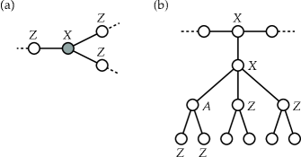
Figure 37: Photon-loss tolerant cluster states. (a) We can measure the Pauli operator $X$ on the shaded (lost) qubit by measuring all the adjacent qubits in the $Z$ basis. (b) Planting a cluster tree using two adjacent $X$ measurements in order to do a single-qubit measurement in the basis $A$.

In cluster-state quantum computing, we need the ability to do single-qubit measurements in an arbitrary basis; $A=\cos\phi\,X+\sin\phi\,Y$. To this end, we use the cluster-state property that two adjacent $X$ measurements remove the qubits from the cluster and transfer the bonds. This way, we can plant the qubit labelled $A$ into the cluster (see Fig. 37b). Instead of doing the $A$ measurement on the in-line qubit, we perform the measurement on a qubit in the third (horizontal) level. When this measurement succeeds, we have to break the bonds with all the other qubits in the tree. Therefore, we measure all the remaining qubits in the third level as well as the qubits in the fourth level that are connected to the $A$ qubit in the $Z$ basis.

Sometimes the photon detection that constitutes the qubit measurement $A$ will fail due to the detector inefficiency. In that case, we can attempt the $A$ measurement on a second qubit in the third level. Again, the remaining qubits and the fourth-level qubits connected to the $A$ qubit must be measured in the $Z$ basis. Whenever such a $Z$ measurement fails (as is the case for the qubit that failed the $A$ measurement), we need to do an indirect $Z$ measurement according to the method outlined above: When a photonic qubit is lost, we need to choose a stabiliser generator for which that photon was represented by a $Z$ operator. The tree structure ensures that such an operator can always be found. We then measure all the photons in this stabiliser generator to establish the $Z$ eigenvalue for the lost photon. In the case of additional photon loss, we repeat this process until we succeed.

When the success probability of the measurement of a logical qubit is given by $p$, then the number of qubits in a tree $n$ is given by

$$n=\mathrm{polylog}\left(\frac{1}{1-p}\right).$$ (117)

Numerical simulations indicate that a detector loss of up to 50% can be corrected Varnava et al. (2005). Moreover, if more than 50% of the photons were allowed to be lost, then we can imagine that all the lost photons are collected by a third party who can perform a measurement complementary to $A$ on the same qubit. Since this would violate various no-cloning bounds, such a strategy must be ruled out. Hence, a detection efficiency of 50% is the absolute minimum Barrett (2005).

In the circuit-based model by Gilchrist, Hayes, and Ralph, the lowest level of encoding consists of a polarised photon such that $|0\rangle\equiv|H\rangle$ and $|1\rangle\equiv|V\rangle$. The second level of encoding is the parity code $\{|0\rangle^{(n)},|1\rangle^{(n)}\}$ of Eq. (81), which allows us to use the probabilistic fusion gates in a deterministic manner. The third level of encoding is a redundant encoding such that a logical qubit is encoded in a GHZ state of parity-encoded qubits Ralph et al. (2005):

$$|\psi\rangle_{L}\equiv\alpha|0\rangle^{(n)}_{1}\ldots|0\rangle^{(n)}_{q}+\beta|1\rangle^{(n)}_{1}\ldots|1\rangle^{(n)}_{q}.$$ (118)

To demonstrate that this code protects quantum information from photon loss, we show that heralded photon loss merely yields a recoverable error, and that we can perform a universal set of deterministic quantum gates on these logical qubits.

First of all, we note that every pair of optical modes that constitutes the lowest level qubit encoding must contain exactly one photon, and no high number counting is required (contrary to the KLM scheme). This is also true for the Browne-Rudolph protocol. We therefore assume that we have bucket detectors with a certain detection efficiency $\eta$ and a negligible dark count rate. The type-I and type-II fusion gates are then no longer (1,1) and (2,1) strategies, respectively. The type-I fusion gate ceases to yield pure output states, while the type-II gate yields a pure output state only if a detector coincidence is found (we assume perfect sources). A failure not only removes the mode that was involved with the PBS, but we should also measure one mode in order to purify the cluster. Hence, the type-II fusion gate with bucket detectors is a (2,2)-strategy, and the growth requirement is $m>2/p$.

Suppose we wish to measure the value of the logical qubit $|\psi\rangle_{L}$ in the computational basis (as we discuss below, any other measurement can be performed by first applying a single-qubit rotation to $|\psi\rangle_{L}$). Since the logical qubit is a GHZ state, it is sufficient to measure only one parity qubit, e.g., the first one. Physically, this measurement constitutes a counting of horizontally and vertically polarised photons: if the number of vertically polarised photons is even, then the value of the parity qubit is $|0\rangle_{1}^{(n)}$, and if it is odd, then its value is $|1\rangle_{1}^{(n)}$. In order to successfully establish the parity, we therefore need to detect all $n$ photons.

When we include photon loss in this measurement, there are three possible measurement outcomes for every optical mode: “horizontal”, “vertical”, or “detector failure”. In the language of POVMs, this can be written as

$$\hat{E}^{(H)} = \eta|H\rangle\langle H|\;;$$ (119)

$$\hat{E}^{(V)} = \eta|V\rangle\langle V|\;;$$ (120)

$$\hat{E}^{(0)} = (1-\eta)\left(|H\rangle\langle H|+|V\rangle\langle V|\right)\;.$$ (121)

These POVMs add up to unity in the subspace spanned by $|H\rangle$ and $|V\rangle$, as required. A particular measurement outcome on $n$ modes can then be written as a string of $n$ outcomes $s=(s_{1},\ldots,s_{n})$, where every $s_{i}\in\{H,V,0\}$. The optical state after finding a particular measurement outcome $s$ is then

$$\rho_{2\ldots q}=\mathrm{Tr}_{1}\left[\hat{E}_{1}^{(s)}|\psi\rangle_{L}\langle\psi|\right]\;.$$ (122)

When all photons are detected, the qubit is projected onto its logical value. However, when one or more qubits are lost it is no longer possible to establish the parity. Therefore, as soon as a photon is lost the next photon is measured in a diagonal basis, thus disentangling the parity qubit from the other parity qubits. A few lines of algebra shows that the remaining $q-1$ parity qubits are in the state

$$|\psi\rangle_{L}^{\prime}=\alpha|0\rangle^{(n)}_{2}\ldots|0\rangle^{(n)}_{q}+\beta|1\rangle^{(n)}_{2}\ldots|1\rangle^{(n)}_{q}.$$ (123)

In other words, the encoding has become smaller but the quantum information has not been erased. We can therefore retry the measurement of the qubit $q$ times.

Next, we have to show that we can perform deterministic one- and two-qubit gates using this redundant encoding. To this end, recall how deterministic gates were implemented in the parity encoding: A universal set of gates is $\{X_{\theta}^{(p)},Z^{(p)},Z_{\pi/2}^{(p)},\mathrm{CNOT}^{(p)}\}$. We added a superscript $(p)$ to indicate that these gates act on the parity qubit. As we have seen, the gates $Z_{\pi/2}^{(p)}$ and CNOT^(p) cannot be implemented deterministically, and have to be built using fusion gates.

How can these gates be used to form a universal set on the redundantly encoded (logical) qubit? First, the single-qubit gate $Z$ is still implemented deterministically: $Z=Z^{(p)}=n\sigma_{z}$. Therefore, in order to apply a $Z$ gate, a $\sigma_{z}$ operation must be applied to all $n$ photons in one and only one parity qubit. Secondly, the gate $Z_{\pi/2}$ is diagonal in the computational basis, and can therefore be implemented using one $Z_{\pi/2}^{(p)}$. Thirdly, the $X_{\theta}$ gate on the redundantly encoded qubit is somewhat problematic, since the gate transforms separable states of parity qubits into highly entangled GHZ states. However, if we apply $(q-1)$ CNOT^(p) gates, we can decode the qubit such that its state is $(\alpha|0\rangle_{1}^{(n)}+\beta|1\rangle_{1}^{(n)})\otimes|0\rangle_{2}^{(n)}\ldots|0\rangle_{q}^{(n)}$. We can then apply the deterministic gate $X_{\theta}^{(p)}$ to the first parity qubit, and use another set of $(q-1)$ CNOT^(p) gates to re-encode the qubit. Therefore, the gate $X_{\theta}$ “costs” $2(q-1)$ CNOT^(p) gates. Finally, the CNOT gate on the redundantly encoded qubit can be implemented using $q$ CNOT^(p) gates.

Since every single-qubit operation can be constructed from $X_{\theta}$ and $Z_{\pi/2}$, we can perform arbitrary single-qubit measurements. We now have a universal set of gates on our logical qubit, together with computational-basis read out and an efficient encoding mechanism. Numerical simulations indicate that this method allows for combined detector, source and memory efficiencies of $\eta>55\%$ Ralph et al. (2005).

Note that there seem to be conflicting requirements in this code: In order to execute successful fusion gates, we want $n$ to be reasonably large. On the other hand, we want $n$ to be as small as possible such that the probability of measuring all $n$ photons $p=\eta^{n}$ is not too small. We assumed that every parity qubit is encoded with the same number of photons $n$, but this is not necessary. In principle, this method works when different parity qubits have different-sized encodings. However, some care should be taken to choose every $n_{i}$ as close to the optimal value as possible.

V.2 General error correction in LOQC

As we mentioned before, photon loss is not the only error in LOQC, and creating large cluster trees or a sizable redundant encoding in the circuit model will actually amplify other errors, such as dephasing. A truly fault-tolerant quantum computer architecture must therefore be able to handle the actual physical noise that will be present. Given a certain noise model and error correcting codes, we can derive fault-tolerant thresholds: The errors must be smaller than the threshold value for concatenated error correction to eliminate them all. Knill et al. (2000) considered a combination of photon loss and dephasing in the original KLM proposal and found that the accuracy threshold for the optical components in that scheme was higher than 99%.

Dawson, Haselgrove, and Nielsen (2006a,b) performed an extensive numerical study of fault-tolerant thresholds for linear optical cluster state quantum computing. The computational model they adopted is Nielsen’s micro-cluster approach, described in section III.3, with type-I fusion gates instead of KLM-type CZ gates. The physical operations in this model are Bell-state preparation, single-photon gates and memories, type-I fusion gates, and photon measurements. The computation proceeds in time steps, with exactly one operation at each step. Furthermore, it is assumed that any two single-photon qubits in the computation can serve as the inputs of the fusion gate. In other words, we have a direct interaction between qubits. In addition, parallel operations are allowed to speed up the computation and minimise the use of quantum memories. Finally, the classical computation needed to control the cluster state computing is taken to be sufficiently fast.

The noise model adopted by Dawson et al. consists of the inherent probabilistic nature of the fusion gates, as well as photon loss and depolarisation at every time step in the computation. The photon loss is characterised by a uniform loss probability $\gamma$, and the depolarisation comes in two flavours: Single-qubit operations have a probability $\epsilon/3$ of undergoing a Pauli operation $X$, $Y$, or $Z$. After the Bell-state preparation and before the fusion gate input, the two photons undergo a correlated depolarising noise: With probability $(1-\epsilon)$ nothing happens to the qubits, while with probability $\epsilon/15$ any of the remaining 15 two-qubit Pauli operators are applied. This is a completely general model for the noise that can affect optical cluster state quantum computing, and the resulting fault-tolerance simulation gives an accuracy threshold region on $\gamma$ and $\epsilon$. Thresholds were obtained for both a seven-qubit CSS error correction code and a 23-qubit Golay error correction code. The study shows that scalable quantum computing with the 23-qubit code is possible for a maximum loss probability of $\gamma<3\cdot 10^{-3}$ and a maximum depolarising probability of $\epsilon<10^{-4}$.

Even though this noise model accounts for general noise, and the fault-tolerant threshold puts a bound on its magnitude, it is clearly a simplification of the physical noise that is expected in cluster state LOQC. It is argued that the difference between correlated two-qubit noise and independent noise does not change the threshold much. Similarly, using one parameter to describe both photon absorption and detector efficiency will not have a dramatic effect on the threshold Nielsen (2006). The next milestone for establishing fault-tolerance thresholds is to adopt a noise model in which the parameters are measurable quantities, such as the visibility in a Hong-Ou-Mandel experiment and photon loss probabilities.

When various parameters in a noise model differ significantly, it might be beneficial to diversify the error correction codes. EC codes that correct specific errors such as photon loss or depolarisation may be smaller than generic EC codes, and therefore introduce less noise. A round of special error correction might be used to reduce large errors, and subsequent generic error correction will further reduce the errors below the fault-tolerant threshold.

In addition, certain types of errors or noise might be naturally suppressed by a suitable alteration in the architecture. For example, there is a way to create high-fidelity four-photon GHZ states with lossy bucket detectors and inefficient sources Gilchrist (2005). Assume that the Bell-pair source creates a state of the form $p_{s}|0\rangle\langle 0|+(1-p_{s})|\Psi^{-}\rangle\langle\Psi^{-}|$, where $|\Psi^{-}\rangle$ is the two-photon polarization singlet state. This is a reasonable error model when the source obeys selection rules that prevent single-photon components to contribute to the output state (c.f., Benson et al. 2000). In order to make a three-photon GHZ state using these sources we use a type-I fusion gate and post-select on a single detector click. The detector click indicates that at least one source created a photon pair. However, if only one photon pair was created, the output mode of the type-I fusion gate must necessarily empty. By taking the output modes of two type-I fusion gates in two separate three-photon GHZ creation attempts, and leading them into a type-II fusion gate, we can post-select on finding two detector clicks. As a result, high-fidelity four-photon GHZ states are produced.

Several other specialised circuits have been proposed that either detect errors or correct them. For example, Ralph (2003) proposed a simple demonstration circuit that detects and corrects bit flip errors on a single qubit using the encoded qubit state $\alpha|0\rangle|0\rangle+\beta|1\rangle|1\rangle$ and an ancilla qubit $|0\rangle$. However, since this is a probabilistic protocol, this circuit cannot naively be inserted in a quantum computing circuit. If we assume the availability of perfectly efficient detectors (not necessarily photon-number resolving), deterministic polarisation-flip detection for distributing entanglement can be achieved Kalamidas (2004). In a similar fashion, a single-qubit error correction circuit can be constructed with polarising beam splitters, half-wave plates, and Pockels cells Kalamidas (2005). Here, we assume that these passive optical elements do not induce additional noise. A full analysis would have to take this noise into account.

VI Outlook: beyond linear optics

We have seen in this review that it is possible to construct a quantum computer with linear optics, single-photon sources, and photon detection alone. Knill, Laflamme, and Milburn (2001) overturned the conventional wisdom that a lack of direct photon-photon interactions prohibits scalability. Since KLM, several groups have proposed modifications to building a linear optical quantum computer with reduced resources and realistic (noisy) components.

The basic principles of LOQC have all been demonstrated experimentally, predominantly using parametric down-conversion (PDC) and bucket photon detection. Due to the small efficiency of PDC photon sources, however, these techniques cannot be considered scalable in a practical sense. Currently, there is a concerted effort to build the necessary single-photon sources, photon detectors, and quantum memories for a scalable linear optical quantum computer. On the theoretical front, there is an ongoing effort to design more efficient architectures and effective error correction codes tailored to the noise model that is relevant to LOQC.

Nevertheless, constructing the necessary components and using fault-tolerant encoding is hard, and several extensions to LOQC have been proposed. In this last section we sketch a few additions to the linear optical toolbox that can make quantum computing a little bit easier.

First, we have seen in section I.4 that a cross-Kerr nonlinearity can be used to induce a photon-photon interaction, and how two-qubit quantum gates can be constructed using such a nonlinearity. Unfortunately, natural Kerr nonlinearities are extremely small, and this is not a practical method for creating optical gates. However, recently it was suggested that a small nonlinearity might still be used for quantum computing. It was shown by Munro et al. (2005) how such nonlinearities can make a number-resolving QND detector, and Barrett et al.  (2005) showed how a small cross-Kerr nonlinearity can be used to perform complete Bell measurements without destroying the photons. Subsequently, it was realized by Nemoto and Munro (2004) that this technique can also be used to create a deterministic CNOT gate on photonic qubits. Recent work in electromagnetically induced transparencies by Lukin and Imamoǧlu (2000, 2001) suggests that the small-but-not-tiny nonlinearities needed for this method are on the threshold of becoming practical. Alternatively, relatively large nonlinearities can be obtained in photonic band-gap materials Friedler et al. (2004).

Secondly, if we have high-fidelity single-photon sources and memories, it might become beneficial to engineer these systems such that they support coherent single-qubit operations. This way, we can redefine our qubits as isolated static systems, and we have circumvented the problem of qubit loss. When these matter qubits emit a qubit-dependent photon, they can in turn be entangled using techniques from linear optical quantum computing. It was shown by Barrett and Kok (2005) that such an architecture can support scalable quantum computing, even with current realistic components. Independently, Lim et al. (2005) showed how a similar setup can be used to implement deterministic two-qubit quantum gates. Recently, these two methods were combined in a fault tolerant, near-deterministic quantum computer architecture Lim et al. 2005a .

Thirdly, Franson, Jacobs, and Pittman proposed the implementation of a two-qubit $\sqrt{\mbox{\sc swap}}$ gate using the quantum Zeno effect: Two optical fibres are fused and split again, such that the input modes overlap in a small section of the fibre. This acts as a beam splitter on the modes in the input and output fibres. At regular intervals inside the joint fibre we place atoms with a two-photon transition. This transition acts as a two-photon measurement, while single-photon wave-packets propagate through the fibre undisturbed. Furthermore, the single-photon wave-packets maintain coherence. The effect of this repeated two-photon measurement is to suppress the Hong-Ou-Mandel effect via the quantum Zeno effect. In this way, two single-photon qubits in the input modes are transformed into two single-photon qubits in the output modes and undergo a $\sqrt{\mbox{\sc swap}}$ gate.

Finally, an alternative approach to linear optical quantum computing involves encoding qubits in squeezed or coherent states of light Gottesman et al. (2001); Ralph et al. (2003). Linear elements take on a new capability in these implementations. For example Bell measurements and fan-out gates become deterministic elements van Enk and Hirota (2002); Jeong et al. (2001). The downside is that it is difficult to produce the superposition states that are required as resources in such schemes, although considerable theoretical and experimental progress has been made recently Lund et al. (2004); Wenger et al. (2004). If this problem is solved, considerable savings in resources could result from adopting such implementations.

Whatever the ultimate architecture of quantum computers will be, there will always remain a task for (linear) optical quantum information processing: In order to distribute quantum information over a network of quantum computers, the qubit of choice will most likely be optical. We therefore believe that the techniques reviewed here are an important step towards full-scale distributed quantum computing — the Quantum Internet.

References

- Achilles et al. (2003) D. Achilles, C. Silberhorn, C. Śliwa, K. Banaszek, and I. A. Walmsley, Opt. Lett., 28 2387, 2003.
- Adami and Cerf (1999) C. Adami and N. J. Cerf, Lect. Notes Comput. Sc., 1509 391, 1999.
- Banaszek and Walmsley (2003) K. Banaszek and I. A. Walmsley, Opt. Lett., 28 52, 2003.
- Barnett et al. (1989) S. M. Barnett, J. Jeffers, A. Gatti, and R. Loudon, Phys. Rev. A, 57 2134, 1989.
- Barreiro et al. (2005) J. T. Barreiro, N. K. Langford, N. A. Peters, and P. G. Kwiat, Phys. Rev. A, 72 060310, 2005.
- Barrett and Kok (2005) S. D. Barrett and P. Kok, Phys. Rev. A, 72 060310, 2005.
- Barrett et al. (2005) S. D. Barrett, P. Kok, K. Nemoto, R. G. Beausoleil, W. J. Munro, and T. P. Spiller, Phys. Rev. A, 72 060302, 2005.
- Barrett (2005) S. D. Barrett, Private communication, 2005.
- Benson et al. (2000) O. Benson, C. Santori, M. Pelton, and Y. Yamamoto, Phys. Rev. Lett., 84 2513, 2000.
- Bergou et al. (2000) J. A. Bergou, M. Hillery, and Y. Q. Sun, J. Mod. Opt., 47 487, 2000.
- Berry et al. (2004) D. W. Berry, S. Scheel, C. R. Meyers, B. C. Sanders, P. L. Knight, and R. Laflamme, New J. Phys., 6 93, 2004.
- Berry et al. (2005) D. W. Berry, S. Scheel, B. C. Sanders, and P. L. Knight, Phys. Rev. A, 69 031806, 2005.
- Beveratos et al. (2002) A. Beveratos, S. Kühn, R. Brouri, T. Gacoin, J. P. Poizat, and P. Grangier, Eur. Phys. J. D, 18 191, 2002.
- Biedenharn and Louck (1981) L. C. Biedenharn and J. D. Louck, Angular Momentum in Quantum Physics (Encyclopedia of Mathematics and Its Applications 8), Addison-Wesley, 1981.
- Boschi et al. (1998) D. Boschi, S. Branca, F. D. Martini, L. Hardy, and S. Popescu, Phys. Rev. Lett., 80 1121, 1998.
- Branczyk et al. (2003) A. M. Branczyk, T. J. Osborne, A. Gilchrist, and T. C. Ralph, Phys. Rev. A, 68 043821, 2003.
- Braunstein and Mann (1996) S. L. Braunstein and A. Mann, Phys. Rev. A, 51 R1727, 1996.
- Braunstein and van Loock (2005) S. L. Braunstein and P. van Loock, Rev. Mod. Phys., 77 513, 2005.
- Brokmann et al. (2004) X. Brokmann, G. Messin, P. Desbiolles, E. Giacobino, M. Dahan, and J. P. Hermier, New J. Phys., 6 99, 2004.
- Browne and Rudolph (2005) D. E. Browne and T. Rudolph, Phys. Rev. Lett., 95 010501, 2005.
- Brune et al. (1990) M. Brune, S. Haroche, V. Lefevre, J. Raimond, and N. Zagury, Phys. Rev. Lett., 65 976, 1990.
- Brune et al. (1992) M. Brune, S. Haroche, J. M. Raimond, L. Davidovich, and N. Zagury, Phys. Rev. A, 45 5193, 1992.
- Brunel et al. (1999) C. Brunel, B. Lounis, P. Tamarat, and M. Orrit, Phys. Rev. Lett., 83 2722, 1999.
- Calsamiglia (2002) J. Calsamiglia, Phys. Rev. A, 65 030301, 2002.
- Cerf et al. (1998) N. J. Cerf, C. Adami, and P. G. Kwiat, Phys. Rev. A, 57 R1477, 1998.
- Chuang and Nielsen (1997) I. L. Chuang and M. A. Nielsen, J. Mod. Phys., 44 2455, 1997.
- Chuang and Yamamoto (1995) I. L. Chuang and Y. Yamamoto, Phys. Rev. A, 52 3489, 1995.
- Cinelli et al. (2005) C. Cinelli, M. Barbieri, F. D. Martini, and P. Mataloni, Laser Phys., 15 124, 2005.
- Clausen et al. (2002) J. Clausen, L. Knöll, and D. G. Welsch, J. Opt. B, 4 155, 2002.
- Clausen et al. (2003) J. Clausen, L. Knöll, and D. G. Welsch, Phys. Rev. A, 68 043822, 2003.
- Clauser and Dowling (1996) J. F. Clauser and J. P. Dowling, Phys. Rev. A, 53 4587, 1996.
- d’Ariano et al. (2000) G. M. d’Ariano, C. Macchiavello, and L. Maccone, Fortschr. Phys., 48 573, 2000.
- (33) C. M. Dawson, H. L. Haselgrove, and M. A. Nielsen, Phys. Rev. Lett., 96 020501, 2006.
- (34) C. M. Dawson, H. L. Haselgrove, and M. A. Nielsen, quant-ph/0601066, 2006.
- De Martini et al. (2005) F. De Martini, G. Di Giuseppe, and M. Marrocco, Phys. Rev. Lett., 76 900, 1996.
- de Riedmatten et al. (2003) H. de Riedmatten, I. Marcikic, W. Tittel, H. Zbinden, and N. Gisin, Phys. Rev. A, 67 022301, 2003.
- (37) P. Deuar and W. J. Munro, Phys. Rev. A, 61 010306, 2000.
- (38) P. Deuar and W. J. Munro, Phys. Rev. A, 62 042304, 2000.
- Dowling (1998) J. P. Dowling, IEEE Proc. Opt. Elec., 145 420, 1998.
- Eisert (2005) J. Eisert, Phys. Rev. Lett., 95 040502, 2005.
- Ekert (1998) A. Ekert, Phys. Scripta, T76 218, 1998.
- Englert et al. (2001) B. G. Englert, C. Kurtsiefer, and H. Weinfurter, Phys. Rev. A, 63 032303, 2001.
- Fearn and Loudon (1987) H. Fearn and R. Loudon, Opt. Commun., 64 485, 1987.
- Fiorentino and Wong (2004) M. Fiorentino and F. N. C. Wong, Phys. Rev. Lett., 93 070502, 2004.
- Fitch et al. (2003) M. J. Fitch, B. C. Jacobs, T. B. Pittman, and J. D. Franson, Phys. Rev. A, 68 043814, 2003.
- Fleischhauer and Lukin (2002) M. Fleischhauer and M. D. Lukin, Phys. Rev. A, 65 022314, 2002.
- Franson and Pittman (1999) J. D. Franson and T. B. Pittman, Lect. Notes Comput. Sc., 1509 383, 1999.
- Franson et al. (2002) J. D. Franson, M. M. Donegan, M. J. F. B. Jacobs, and T. B. Pittman, Phys. Rev. Lett., 89 137901, 2002.
- Franson et al. (2003) J. D. Franson, B. C. Jacobs, and T. B. Pittman, Fortschr. Phys., 51 369, 2003.
- Friedler et al. (2004) I. Friedler, G. Kurizki, and D. Petrosyan, Europhys. Lett., 68 625, 2004.
- Gaebel et al. (2004) T. Gaebel, I. Popa, A. Gruber, M. Domhan, F. Jelezko, and J. Wrachtrup, N. J. Phys., 6 98, 2004.
- Gasparoni et al. (2004) S. Gasparoni, J. W. Pan, P. Walther, T. Rudolph, and A. Zeilinger, Phys. Rev. Lett., 93 020504, 2004.
- Gérard et al. (2002) J. M. Gérard, I. Robert, E. Moreau, M. Gallart, and I. Abram, J. Phys. IV, 12 29, 2002.
- Giacomini et al. (2003) S. Giacomini, F. Sciarrino, E. Lombardi, and F. De Martini, Phys. Rev. A, 66 030302, 2002.
- Gilchrist (2005) A. Gilchrist, private communication to Dan E. Browne.
- Gilchrist et al. (2003) A. Gilchrist, W. J. Munro, and A. G. White, Phys. Rev. A, 67 040304, 2003.
- Gilchrist et al. (2005) A. Gilchrist, A. J. F. Hayes, and T. C. Ralph, quant-ph/0505125, 2005.
- Gingrich et al. (2003) R. M. Gingrich, P. Kok, H. Lee, F. Vatan, and J. P. Dowling, Phys. Rev. Lett., 91 217901, 2003.
- Glancy et al. (2002) S. Glancy, J. M. LoSecco, H. M. Vasconcelos, and C. E. Tanner, Phys. Rev. A, 65 062317, 2002.
- Gottesman and Chuang (1999) D. Gottesman and I. L. Chuang, Nature, 402 390, 1999.
- Gottesman et al. (2001) D. Gottesman, A. Kitaev, and J. Preskill, Phys. Rev. A, 64 012310, 2001.
- Gottesman (1999) D. Gottesman, The Heisenberg Representation of Quantum Computers, Group 22: Proceedings of the XXII International Colloquium on Group Theoretical Methods in Physics, Cambridge, MA, International Press, 1999.
- Grangier et al. (1998) P. Grangier, J. A. Levenson, and J. P. Poizat, Nature, 396 537, 1998.
- Greulich and Thiel (2001) K. O. Greulich and E. Thiel, Single Mol., 2 5, 2001.
- Grice et al. (2001) W. P. Grice, A. B. U’Ren, and I. A. Walmsley, Phys. Rev. A, 64 063815, 2001.
- Hayes et al. (2004) A. J. F. Hayes, A. Gilchrist, C. R. Myers, and T. C. Ralph, J. Opt. B, 6 533, 2004.
- Hein et al. (2004) M. Hein, J. Eisert, and H. J. Briegel, Phys. Rev. A, 69 062311, 2004.
- Hennrich et al. (2004) M. Hennrich, T. Legero, A. Kuhn, and G. Rempe, New J. Phys., 6 86, 2004.
- Hockney et al. (2003) G. M. Hockney, P. Kok, and J. P. Dowling, Phys. Rev. A, 67 032306, 2003.
- Hofmann and Takeuchi (2002) H. F. Hofmann and S. Takeuchi, Phys. Rev. A, 66 024308, 2002.
- Hofmann et al. (2003) H. F. Hofmann, K. Kojima, S. Takeuchi, and K. Sasaki, J. Opt. B, 5 218, 2003.
- Hollars et al. (2003) C. W. Hollars, S. M. Lane, and T. Huser, Chem. Phys. Lett., 370 393, 2003.
- Hong et al. (1987) C. K. Hong, Z. Y. Ou, and L. Mandel, Phys. Rev. Lett., 59 2044, 1987.
- Hours et al. (2003) J. Hours, S. Varoutsis, M. Gallart, J. Bloch, I. Robert-Philip, A. Cavanna, I. Abram, F. Laruelle, and J. M. Gérard, Appl. Phys. Lett., 82 2206, 2003.
- (75) J. C. Howell and J. A. Yeazell, Phys. Rev. A, 62 032311, 2000.
- (76) J. C. Howell and J. A. Yeazell, Phys. Rev. Lett., 85 198, 2000.
- (77) J. C. Howell and J. A. Yeazell, Phys. Rev. A, 61 052303, 2000.
- Hutchinson and Milburn (2004) G. D. Hutchinson and G. J. Milburn, J. Mod. Opt., 51 1211, 2004.
- Imamoǧlu (2002) A. Imamoǧlu, Phys. Rev. Lett., 89 163602, 2002.
- Imoto et al. (1985) N. Imoto, H. A. Haus, and Y. Yamamoto, Phys. Rev. A, 32 2287, 1985.
- Jacobs et al. (2002) B. C. Jacobs, T. B. Pittman, and J. D. Franson, Phys. Rev. A, 66 052307, 2002.
- James and Kwiat (2002) D. F. V. James and P. G. Kwiat, Phys. Rev. Lett., 89 183601, 2002.
- Jelezko et al. (2002) F. Jelezko, I. Popa, A. Gruber, C. Tietz, and J. Wrachtrup, Appl. Phys. Lett., 81 2160, 2002.
- Jeong et al. (2001) H. Jeong, M. S. Kim, and J. Lee, Phys. Rev. A, 64 052308, 2001.
- Jex et al. (1995) I. Jex, S. Stenholm, and A. Zeilinger, Opt. Commun., 117 95, 1995.
- Johnsson and Fleischhauer (2003) M. Johnsson and M. Fleischhauer, Phys. Rev. A, 67 061802, 2003.
- Julsgaard et al. (2004) B. Julsgaard, J. Sherson, J. I. Cirac, J. Fiurášek, and E. S. Polzik, Nature, 432 482, 2004.
- Kalamidas (2004) D. Kalamidas, Phys. Lett. A, 321 87, 2004.
- Kalamidas (2005) D. Kalamidas, Phys. Lett. A, 343 331, 2005.
- Keller et al. (2004) M. Keller, B. Lange, K. Hayasaka, W. Lange, and H. Walther, Nature, 431 1075, 2004.
- Kim et al. (1999) J. Kim, S. Takeuchi, Y. Yamamoto, and H. H. Hogue, Appl. Phys. Lett., 74 902, 1999.
- Kiraz et al. (2004) A. Kiraz, M. Atatüre, and A. Imamoǧlu, Phys. Rev. A, 69 032305, 2004.
- Knill et al. (2000) E. Knill, R. Laflamme, and G. J. Milburn, quant-ph/0006120, 2000.
- Knill et al. (2001) E. Knill, R. Laflamme, and G. J. Milburn, Nature, 409 46, 2001.
- Knill (2002) E. Knill, Phys. Rev. A, 66 052306, 2002.
- Knill (2003) E. Knill, Phys. Rev. A, 68 064303, 2003.
- Knill (2005) E. Knill, Nature, 434 39, 2005.
- Koashi et al. (2001) M. Koashi, T. Yamamoto, and N. Imoto, Phys. Rev. A, 63 030301, 2001.
- (99) P. Kok and S. L. Braunstein, Phys. Rev. A, 62 064301, 2000.
- (100) P. Kok and S. L. Braunstein, Phys. Rev. A, 61 042304, 2000.
- Kok and Braunstein (2001) P. Kok and S. L. Braunstein, Phys. Rev. A, 63 033812, 2001.
- Kok and Braunstein (2006) P. Kok and S. L. Braunstein, International Journal of Quantum Information (in press), quant-ph/0407259.
- Kok and Munro (2005) P. Kok and W. J. Munro, Phys. Rev. Lett., 95 048901, 2005.
- Kok et al. (2002) P. Kok, H. Lee, and J. P. Dowling, Phys. Rev. A, 66 063814, 2002.
- Kok (2003) P. Kok, IEEE: Sel. Top. Quantum Electronics, 9 1498, 2003.
- Kuhn et al. (2002) A. Kuhn, M. Hennrich, and G. Rempe, Phys. Rev. Lett., 89 067901, 2002.
- Kurtsiefer et al. (2000) C. Kurtsiefer, S. Mayer, P. Zarda, and H. Weinfurter, Phys. Rev. Lett., 85 290, 2000.
- Kuzmich et al. (2003) A. Kuzmich, W. P. Bowen, A. D. Boozer, A. Boca, C. W. Chou, L. M. Duan, and H. J. Kimble, Nature, 423 731, 2003.
- Kwiat and Weinfurter (1998) P. G. Kwiat and H. Weinfurter, Phys. Rev. A, 58 R2623, 1998.
- Kwiat et al. (2000) P. G. Kwiat, J. R. Mitchell, P. D. D. Schwindt, and A. G. White, J. Mod. Opt., 47 257, 2000.
- Lapaire et al. (2003) G. G. Lapaire, P. Kok, J. P. Dowling, and J. E. Sipe, Phys. Rev. A, 68 042314, 2003.
- (112) H. Lee, U. Yurtsever, P. Kok, G. M. Hockney, C. Adami, S. L. Braunstein, and J. P. Dowling, J. Mod Opt., 51 1517, 2004.
- (113) T. H. Lee, P. Kumar, A. Mehta, K. Xu, R. M. Dickson, and M. D. Barnes, Appl. Phys. Lett., 85 100, 2004.
- Leonhardt and Neumaier (2004) U. Leonhardt and A. Neumaier, J. Opt. B, 6 L1, 2004.
- Leonhardt (2003) U. Leonhardt, Rep. Prog. Phys., 66 1207, 2003.
- Leung (2004) D. W. Leung, Int. J. Quant. Inf., 2 33, 2004.
- Li et al. (2005) X. Li, P. L. Voss, J. Chen, J. E. Sharping, and P. Kumar, Opt. Lett., 30 1201, 2005.
- (118) Y. L. Lim, S. D. Barrett, A. Beige, P. Kok, and L. C. Kwek, Phys. Rev. A, 73 012304, 2006.
- (119) Y. L. Lim, A. Beige, and L. C. Kwek, Phys. Rev. Lett., 95 030505, 2005.
- Lloyd (1995) S. Lloyd, Phys. Rev. Lett, 75 346, 1995.
- Lombardi et al. (2002) E. Lombardi, F. Sciarrino, S. Popescu, and F. De Martini, Phys. Rev. Lett, 88 070402, 2002.
- Lounis and Moerner (2000) B. Lounis and W. E. Moerner, Nature, 407 491, 2000.
- Lounis and Orrit (2005) B. Lounis and M. Orrit, Rep. Prog. Phys., 68 1129, 2005.
- Lounis et al. (2000) B. Lounis, H. A. Bechtel, D. Gerion, P. Alivisatos, and W. E. Moerner, Chem. Phys. Lett.., 329 399, 2000.
- Lukin and Imamoǧlu (2000) M. D. Lukin and A. Imamoǧlu, Phys. Rev. Lett., 84 1419, 2000.
- Lukin and Imamoǧlu (2001) M. D. Lukin and A. Imamoǧlu, Nature, 413 273, 2001.
- Lund and Ralph (2002) A. P. Lund and T. C. Ralph, Phys. Rev. A, 66 032307, 2002.
- Lund et al. (2003) A. P. Lund, T. B. Bell, and T. C. Ralph, Phys. Rev. A, 68 022313, 2003.
- Lund et al. (2004) A. P. Lund, H. Jeong, T. C. Ralph, and M. S. Kim, Phys. Rev. A, 70 020101, 2004.
- Lütkenhaus et al. (1999) N. Lütkenhaus, J. Calsamiglia, and K. A. Suominen, Phys. Rev. A, 59 3295, 1999.
- Lvovsky and Raymer (1999) A. I. Lvovsky and M. G. Raymer, quant-ph/0511044, 2005.
- Maître et al. (1997) X. Maître, E. Hagley, G. Nogues, C. Wunderlich, P. Goy, M. Brune, J. M. Raimond, and S. Haroche, Phys. Rev. Lett., 79 769, 1997.
- Maurer et al. (2004) C. Maurer, C. Becher, C. Russo, J. Eschner, and R. Blatt, New J. Phys., 6 94, 2004.
- McKeefer et al. (2004) J. McKeefer, A. Boca, A. D. Boozer, R. Miller, J. R. Buck, A. Kuzmich, and H. J. Kimble, Science, 303 1992, 2004.
- Messin et al. (2001) G. Messin, J. P. Hermier, E. Giacobino, P. Desboilles, and M. Dahan, Opt. Lett., 26 1891, 2001.
- Michler et al. (2000) P. Michler, A. Kiraz, C. Becher, W. V. Schoenfeld, P. Petroff, L. D. Zhang, E. Hu, and A. Imamoǧlu, Science, 290 2282, 2000.
- Migdall et al. (2002) A. L. Migdall, D. Branning, and S. Castelletto, Phys. Rev. A, 66 053805, 2002.
- Milburn (1989) G. J. Milburn, Phys. Rev. Lett., 62 2124, 1989.
- Moreau et al. (2001) E. Moreau, I. Robert, L. Manin, V. Thierry-Mieg, J. M. Gérard, and I. Abram, Phys. Rev. Lett., 87 183601, 2001.
- Munro et al. (2005) W. J. Munro, K. Nemoto, R. G. Beausoleil, and T. P. Spiller, Phys. Rev. A, 71 033819, 2005.
- Myers and Brandt (1997) J. M. Myers and H. E. Brandt, Meas. Sci, Technol., 8 1222, 1997.
- (142) C. R. Myers and R. Laflamme, Lecture notes for the International School of Physics “Enrico Fermi” on “Quantum Computers, Algorithms and Chaos”, Varenna, Italy, 2005; quant-ph/0512104.
- Nemoto and Braunstein (2002) K. Nemoto and S. L. Braunstein, Phys. Rev. A, 66 032306, 2002.
- Nemoto and Munro (2004) K. Nemoto and W. J. Munro, Phys. Rev. Lett., 93 250502, 2004.
- Newton and Wigner (1949) T. D. Newton and E. P. Wigner, Rev. Mod. Phys., 21 400, 1949.
- Nielsen and Chuang (2000) M. A. Nielsen and I. L. Chuang, Quantum Computation and Quantum Information, Cambridge University Press, 2000.
- Nielsen and Dawson (2004) M. A. Nielsen and C. M. Dawson, Phys. Rev. A, 71 042323, 2004.
- Nielsen (2003) M. A. Nielsen, Phys. Lett. A, 308 96, 2003.
- Nielsen (2004) M. A. Nielsen, Phys. Rev. Lett., 93 040503, 2004.
- Nielsen (2005) M. A. Nielsen, quant-ph/0504097, 2005.
- Nielsen (2006) M. A. Nielsen, private communication.
- Nogues et al. (1999) G. Nogues, A. Rauschenbeutel, S. Osnaghi, M. Brune, J. M. Raimond, and S. Haroche, Nature, 400 239, 1999.
- O’Brien et al. (2003) J. L. O’Brien, G. J. Pryde, A. G. White, T. C. Ralph, and D. Branning, Nature, 426 264, 2003.
- O’Brien et al. (2004) J. L. O’Brien, G. J. Pryde, A. Gilchrist, D. F. V. James, N. K. Langford, T. C. Ralph, and A. G. White, Phys. Rev. Lett., 93 080502, 2004.
- O’Brien et al. (2005) J. L. O’Brien, G. J. Pryde, A. G. White, and T. C. Ralph, Phys. Rev. A, 71 060303, 2005.
- Paris et al. (2003) M. G. A. Paris, G. M. d’Ariano, P. L. Presti, and P. Perinotti, Fortschr. Phys., 51 449, 2003.
- Paris (2000) M. G. A. Paris, Phys. Rev. A, 62 033813, 2000.
- Pelton et al. (2002) M. Pelton, C. Santori, J. Vučković, B. Y. Zhang, G. S. Solomon, J. Plant, and Y. Yamamoto, Phys. Rev. Lett., 89 233602, 2002.
- Peres and Terno (2002) A. Peres and D. R. Terno J. Mod. Opt., 50 1165, 2003.
- Pittman and Franson (2002) T. B. Pittman and J. D. Franson, Phys. Rev. A, 66 062302, 2002.
- (161) T. B. Pittman, B. C. Jacobs, and J. D. Franson, Phys. Rev. A, 66 052305, 2002.
- (162) T. B. Pittman, B. C. Jacobs, and J. D. Franson, Phys. Rev. Lett., 88 257902, 2002.
- (163) T. B. Pittman, B. C. Jacobs, and J. D. Franson, Phys. Rev. A, 66 042303, 2002.
- Pittman et al. (2003) T. B. Pittman, M. J. Fitch, B. C. Jacobs, and J. D. Franson, Phys. Rev. A, 68 032316, 2003.
- Pittman et al. (2005) T. B. Pittman, B. C. Jacobs, and J. D. Franson, Phys. Rev. A, 71 052332, 2005.
- Pittmann et al. (2001) T. B. Pittmann, B. C. Jacobs, and J. D. Franson, Phys. Rev. A, 64 062311, 2001.
- Popescu (1995) S. Popescu, quant-ph/9501020, 1995.
- Poyatos et al. (2001) J. F. Poyatos, J. I. Cirac, and P. Zoller, Phys. Rev. Lett., 78 390, 1997.
- Pryde et al. (2004) G. J. Pryde, J. L. O’Brien, A. G. White, S. D. Bartlett, and T. C. Ralph, Phys. Rev. Lett., 92 190402, 2004.
- Pryde et al. (2005) G. J. Pryde, J. L. O’Brien, A. G. White, S. D. Bartlett, and T. C. Ralph, Phys. Rev. Lett., 95 048902, 2005.
- (171) T. C. Ralph, N. K. Langford, T. B. Bell, and A. G. White, Phys. Rev. A, 65 062324, 2002.
- (172) T. C. Ralph, A. G. White, W. J. Munro, and G. J. Milburn, Phys. Rev. A, 65 012314, 2002.
- Ralph et al. (2003) T. C. Ralph, A. Gilchrist, G. Milburn, W. Munro, and S. Glancy, Phys. Rev. A, 68 042319, 2003.
- Ralph et al. (2005) T. C. Ralph, A. J. F. Hayes, and A. Gilchrist, Phys. Rev. Lett., 95 100501, 2005.
- Ralph (2003) T. C. Ralph, IEEE Sel. Top. Quantum Electronics, 9 1495, 2003.
- Ralph (2004) T. C. Ralph, Phys. Rev. A, 70 012312, 2004.
- Raussendorf and Briegel (2001) R. Raussendorf and H. J. Briegel, Phys. Rev. Lett., 86 5188, 2001.
- Raussendorf et al. (2003) R. Raussendorf, D. E. Browne, and H. J. Briegel, Phys. Rev. A, 68 022312, 2003.
- Raymer et al. (2005) M. G. Raymer, J. Noh, K. Banaszek, and I. A. Walmsley, Phys. Rev. A, 72 023825, 2005.
- Reck et al. (1994) M. Reck, A. Zeilinger, H. J. Bernstein, and P. Bertani, Phys. Rev. Lett., 73 58, 1994.
- Resch et al. (2002) K. J. Resch, J. S. Lundeen, and A. M. Steinberg, Phys. Rev. Lett., 89 037904, 2002.
- Roch et al. (1997) J. F. Roch, K. Vigneron, P. Grelu, A. Sinatra, J. P. Poizat, and P. Grangier, Phys. Rev. Lett., 78 634, 1997.
- Rohde and Ralph (2005) P. P. Rohde and T. C. Ralph, Phys. Rev. A, 71 032320, 2005.
- Rohde et al. (2005) P. P. Rohde, T. C. Ralph, and M. A. Nielsen Phys. Rev. A, 72 052332, 2005.
- Rohde (2005) P. P. Rohde, J. Opt. B, 7 82, 2005.
- Rosenberg et al. (2005) D. Rosenberg, A. E. Lita, A. J. Miller, and S. W. Nam, Phys. Rev. A, 71 061803, 2005.
- Rudolph and Pan (2001) T. Rudolph and J. W. Pan, quant-ph/0108056, 2001.
- Sanaka et al. (2004) K. Sanaka, T. Jennewein, J. W. Pan, K. Resch, and A. Zeilinger, Phys. Rev. Lett., 92 017902, 2004.
- Sanders and Rice (2000) B. C. Sanders and D. A. Rice, Phys. Rev. A, 61 013805, 2000.
- Santori et al. (2001) C. Santori, M. Pelton, G. S. Solomon, Y. Dale, and Y. Yamamoto, Phys. Rev. Lett., 86 1502, 2001.
- (191) C. Santori, D. Fattal, M. Pelton, G. S. Solomon, and Y. Yamamoto, Phys. Rev. B, 66 045308, 2002.
- (192) C. Santori, D. Fattal, J. Vučković, G. S. Solomon, and Y. Yamamoto, Nature, 419 594, 2002.
- Santori et al. (2004) C. Santori, D. Fattal, J. Vučković, G. S. Solomon, and Y. Yamamoto, New J. Phys., 6 89, 2004.
- Scheel and Audenaert (2005) S. Scheel and K. M. R. Audenaert, New J. Phys., 7 149, 2005.
- Scheel and Lütkenhaus (2004) S. Scheel and N. Lütkenhaus, New J. Phys., 6 51, 2004.
- Scheel et al. (2003) S. Scheel, K. Nemoto, W. J. Munro, and P. L. Knight, Phys. Rev. A, 68 032310, 2003.
- Scheel et al. (2004) S. Scheel, J. Pachos, E. A. Hinds, and P. L. Knight, quant-ph/0403152, 2004.
- Scheel et al. (2005) S. Scheel, W. J. Munro, J. Eisert, K. Nemoto, and P. Kok, Phys. Rev. A, 73 034301, 2006.
- Scheel (2004) S. Scheel, quant-ph/0508189, 2005.
- Scheel (2004) S. Scheel, quant-ph/0406127, 2005.
- Schmidt and Imamoǧlu (1996) H. Schmidt and A. Imamoǧlu, Opt. Lett., 21 1936, 1996.
- Scully and Lamb (1969) M. O. Scully and W. E. Lamb, Phys. Rev., 179 368, 1969.
- Silva et al. (2005) M. Silva, M. Rötteler, and C. Zalka, Phys. Rev. A, 72 032307, 2005.
- Simon and Mukunda (1990) R. Simon and N. Mukunda, Phys. Lett. A, 143 165, 1990.
- Śliwa and Banaszek (2003) C. Śliwa and K. Banaszek, Phys. Rev. A, 67 030101, 2003.
- Spedalieri et al. (2005) F. M. Spedalieri, H. Lee, and J. P. Dowling, Phys. Rev. A, 73 012334, 2006.
- Spiller et al. (2005) T. P. Spiller, W. J. Munro, S. D. Barrett, and P. Kok, Cont. Phys., in press, 2005.
- Spreeuw (1998) R. J. C. Spreeuw, Found. Phys., 28 361, 1998.
- Stace et al. (2003) T. M. Stace, G. J. Milburn, and C. H. W. Barnes, Phys. Rev. B, 67 085317, 2003.
- Steane (2003) A. M. Steane, Phys. Rev. A, 68 042322, 2003.
- Stenholm (1996) S. Stenholm, Opt. Commun., 123 287, 1996.
- Summhammer (1997) J. Summhammer, Phys. Rev. A, 56 4324, 1997.
- Takeuchi et al. (1999) S. Takeuchi, J. Kim, Y. Yamamoto, and H. H. Hogue, Appl. Phys. Lett., 74 1063, 1999.
- (214) S. Takeuchi, Phys. Rev. A, 61 052302, 2000.
- (215) S. Takeuchi, Phys. Rev. A, 62 032301, 2000.
- Takeuchi (2001) S. Takeuchi, Electron. Comm. Jpn. 3, 84 52, 2001.
- Thew et al. (2002) R. T. Thew, S. Tanzilli, W. Tittel, H. Zbinden, and N. Gisin, Phys. Rev. A, 66 062304, 2002.
- Törmä and Stenholm (1996) P. Törmä and S. Stenholm, Phys. Rev. A, 54 4701, 1996.
- Törmä et al. (1995) P. Törmä, S. Stenholm, and I. Jex, Phys. Rev. A, 52 4853, 1995.
- Törmä et al. (1996) P. Törmä, I. Jex, and S. Stenholm, J. Mod. Opt., 43 245, 1996.
- Treussart et al. (2002) F. Treussart, R. Alléaume, V. L. Floc’h, L. T. Xiao, J. M. Courty, and J. F. Roch, Phys. Rev. Lett., 89 093601, 2002.
- Turchette et al. (1995) Q. A. Turchette, C. J. Hood, W. Lange, H. Mabuchi, and H. J. Kimble, Phys. Rev. Lett., 75 4710, 1995.
- U’Ren et al. (2003) A. B. U’Ren, K. Banaszek, and I. A. Walmsley, Quant. Inf. Comput., 3 480, 2003.
- Vaidman and Yoran (1999) L. Vaidman and N. Yoran, Phys. Rev. A, 59 116, 1999.
- van Enk and Hirota (2002) S. J. van Enk and O. Hirota, Phys. Rev. A, 64 022313, 2002.
- van Loock and Lütkenhaus (2004) P. van Loock and N. Lütkenhaus, Phys. Rev. A, 69 012302, 2004.
- Varnava et al. (2005) M. Varnava, D. E. Browne, and T. Rudolph, quant-ph/0507036, 2005.
- Verstraete and Cirac (2004) F. Verstraete and J. I. Cirac, Phys. Rev. A, 70 060302, 2004.
- Vučković et al. (2003) J. Vučković, D. Fattal, C. Santori, and G. S. Solomon, Appl. Phys. Lett., 82 3596, 2003.
- Waks et al. (2003) E. Waks, K. Inoue, W. D. Oliver, E. Diamanti, and Y. Yamamoto, IEEE: J. Sel. Top. Quantum Electron., 9 1502, 2003.
- Walther et al. (2005) P. Walther, K. J. Resch, T. Rudolph, H. Weinfurter, V. Vedral, M. Aspelmeyer, and A. Zeilinger, Nature, 434 169, 2005.
- Ward et al. (2005) M. B. Ward, O. Z. Karimov, D. C. Unitt, Z. L. Yuan, P. See, D. G. Gevaux, A. J. Shields, P. Atkinson, and D. A. Ritchie, Appl. Phys. Lett., 86 201111, 2005.
- Weihs et al. (1996) G. Weihs, M. Reck, H. Weinfurter, and A. Zeilinger, Opt. Lett., 21 302, 1996.
- Weinfurter (1994) H. Weinfurter, Europhysics Lett., 25 559, 1994.
- Wenger et al. (2004) J. Wenger, R. Tualle-Brouri, and P. Grangier, Phys. Rev. Lett., 92 153601, 2004.
- Wightman (1962) A. S. Wightman, Rev. Mod. Phys., 34 845, 1962.
- Yamamoto et al. (1988) Y. Yamamoto, M. Kitagawa, and K. Igeta, Proceedings of the 3rd Asia-Pacific Physics Conference, World Scientific, Singapore, 1988.
- Yamamoto et al. (2003) T. Yamamoto, M. Koashi, Ş. Özdemir, and N. Imoto, Nature, 421 343, 2003.
- Yoran and Reznik (2003) N. Yoran and B. Reznik, Phys. Rev. Lett., 91 037903, 2003.
- Yuan et al. (2002) Z. L. Yuan, B. E. Kardynal, R. M. Stevenson, A. J. Shields, C. J. Lobo, K. Cooper, N. S. Beattie, D. A. Ritchie, and M. Pepper, Science, 295 102, 2002.
- Zeilinger (1981) A. Zeilinger, Am. J. Phys., 49 882, 1981.
- Zhao et al. (2005) Z. Zhao, A. N. Zhang, Y. A. Chen, H. Zhang, J. F. Du, T. Yang, and J. W. Pan, Phys. Rev. Lett., 94 030501, 2005.
- Zou et al. (2002) X. B. Zou, K. Pahlke, and W. Mathis, Phys. Rev. A, 65 064305, 2002.
- Zwiller et al. (2003) V. Zwiller, T. Aichele, W. Seifert, J. Persson, and O. Benson, Appl. Phys. Lett., 82 1509, 2003.