Decay of Quantum Accelerator Modes.

Abstract

Experimentally observable Quantum Accelerator Modes are used as a test case for the study of some general aspects of quantum decay from classical stable islands immersed in a chaotic sea. The modes are shown to correspond to metastable states, analogous to the Wannier-Stark resonances. Different regimes of tunneling, marked by different quantitative dependence of the lifetimes on $1/\hbar$, are identified, depending on the resolution of KAM substructures that is achieved on the scale of $\hbar$. The theory of Resonance Assisted Tunneling introduced by Brodier, Schlagheck, and Ullmo BSU02 , is revisited, and found to well describe decay whenever applicable.

I Introduction.

Classical Hamiltonian systems generically display mixed phase spaces, where regions of regular motion and regions of chaotic motion coexist LL92 . Although no classical transport is allowed between different, disjoint regions, quantum transport is made possible by so-called ”dynamical tunneling”, which allows wave-packets to leak through classical invariant curves. In the case of a wave-packet initially localized inside a classical stable island, a transfer of probability into the chaotic region arises, that may continue a long time, and thus take the form of irreversible decay from the island, whenever $\hbar$ is so small that the Heisenberg time related to fast chaotic diffusion is much larger than the period(s) of regular motion in the island. Islands of regular motion have been found to play crucial roles in many contexts, such as optical cavities oc , driven cold atoms aop , where they have inspired detailed theoretical analysis nimrod , and billiards , where they motivated mathematical investigations vered and atom-optical experimental realizations davidson . Wide attention has been attracted by Chaos Assisted Tunneling, which denotes transmission between symmetry-related islands, across a chaotic region cat . Slow tunneling out of islands dominates the dynamical localization properties in some extended systems iomin ; BKM05 .
In this paper we explore decay from regular islands into the surrounding chaotic regions, which is a central theoretical issue in all the above hinted subjects. It is an appealing idea that decay rates may be estimated, using only information drawn from the structure of classical islands. On account of the ubiquitous character of mixed phase spaces, this theoretical programme is attracting significant attention BSU02 ; NP03 ; BKM05 ; ES05 . In this paper we address the problem in a special case, which has a direct experimental relevance. The Quantum Accelerator Modes (QAM) were experimentally discovered when cold caesium atoms, falling under the action of gravity, were periodically pulsed in time by a standing wave of light Ox99 ; DSFG . The theory of this phenomenon FGR00 shows that the dynamics of an atom is described, in an appropriate gauge, by a formal quantization of either of the classical maps :

$${J}_{t+1}={J}_{t}+{\tilde{k}}\sin(\theta_{t+1})\pm 2\pi\Omega\;\;\;,\;\;\theta_{t+1}=\theta_{t}\pm{J}_{t}\;\;\mbox{\rm mod}(2\pi)\;.$$ (1)

The classical phase portraits exhibit periodic (in $J$) chains of regular islands. The rest of phase space is chaotic, and QAMs are produced whenever an atomic wavepacket is at least partially trapped inside the islands. Therefore, QAMs eventually decay in time, due to quantum tunneling FGR00 . The problem of QAMs has a relation to the famous Wannier-Stark problem GRF05 about motion of a particle under the combined action of a constant and a periodic in space force field GKK02 , and the class of QAMs we consider in this paper are due to metastable states nimrod , which are analogous to the Wannier-Stark resonances, and are associated with sub-unitary eigenvalues of the Floquet evolution operator. We derive and numerically support quasi-classical, order-of-magnitude estimates for their decay rates, based on classical phase-space structures. We theoretically and numerically demonstrate that decay is determined by different types of tunneling, depending on how significant the KAM structures inside the island are on the scale of $\hbar$, and in particular we show that these different mechanisms result in different quantitative dependence on the basic quasi-classical parameter given by ${\cal A}/\hbar$, where $\cal A$ is the area of an island. In the regime where higher-order structures inside the island are quantally resolved, we use the theory of Resonance Assisted Tunneling BSU02 to describe the decay of QAMs and find a good agreement in the presence of a single dominant resonance. In particular we observe, in especially clean form , a remarkable stepwise dependence on the quasi-classical parameter, as first predicted in BSU02 .
The phase space islands which are studied in this paper are directly related to experiments on laser cooled atomsOx99 ; DSFG . Unfortunately the step structure which is here predicted occurs in parameter ranges where the decay rate is extremely small. Finding parameter ranges where decay rates are appreciable, and still exhibit step dependence, is a challenging task for experimental application.

II Classical and Quantum dynamics.

QAMs one-to-one correspond to stable periodic orbits of the map on the 2-torus which is obtained from (1) on reading $J$ modulo $(2\pi)$ GRF05 FGR00 . This class of orbits in particular includes fixed points (i.e., period-1 orbits) of map (1). It is these period-1 orbits that give rise to the most clearly observable QAMs, and in this paper we restrict to them . Map (1) differs from the Standard Map only because of the drift $2\pi\Omega$ in the 1st equation. Despite its formal simplicity, this variant introduces nontrivial problems, concerning Hamiltonian formulation and quantization, which are discussed in this section.

II.1 Wannier-Stark pendulum.

Let ${\tilde{k}}=k\epsilon$ and $2\pi\Omega=a\epsilon$, with $\epsilon$ a small parameter. For $\epsilon=0$, map (1) has circles of fixed points at the ”resonant” values of the action ${J}=2\pi s$, $(s\in{\mathbb{Z}})$. Straightforward calculation shows that for $\epsilon>0$ a stable fixed point, surrounded by a stable island, survives near each resonant action, whenever $k$ is larger than $a$ and smaller than a stability border FGR00 . Other islands , related to periodic orbits of higher periods, may or may not significantly coexist with such period-1 islands, depending on parameter values. In any case, numerical simulation shows that motion outside all such islands is essentially chaotic at any $\epsilon>0$.
Using canonical perturbation theory, one finds GRF05 that in the vicinity of resonant actions, and at 1st order in $\epsilon$, the dynamics (1) are canonically conjugate to the dynamics which are locally ruled by the ”resonant Hamiltonian”:

$$H_{res}({\cal J},\vartheta)=\frac{1}{2}{\cal J}^{2}+\epsilon V(\vartheta)\;\;\;;\;\;V(\vartheta)=-a\vartheta+k\cos(\vartheta)\;.$$ (2)

Multivaluedness of $V(\vartheta)$ is removed on taking derivatives, so Hamilton’s equations are well-defined on the cylinder, even though the Hamiltonian (2) is not. They uniquely define a ”locally Hamiltonian” flow on the cylinder, which will be termed the Wannier-Stark (WS) pendulum, because, if $\vartheta$ were a linear coordinate and not an angle , then (2) would be the Wannier-Stark (classical) Hamiltonian for 1-dimensional motion of a particle in a sinusoidal potential combined with a static electric field GKK02 . Trajectories of the Wannier-Stark pendulum are obtained, by winding around the circle the trajectories which are defined on the line by the Wannier-Stark Hamiltonian.
If $a=0$, (2) is the Hamiltonian of a standard pendulum, and motion is completely integrable in either of the two regions in which phase space is divided by the pendulum separatrix.

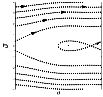
Figure 1: Stable and unstable manifolds of a Wannier-Stark pendulum (2) with $a\epsilon=0.5$ and $k\epsilon=0.7$. On the cylinder, arrows lie on a single continuous trajectory.

If $a\neq 0$ this is not true anymore. In particular, if $|a|<|k|$ then the flow has one stable and one unstable fixed point. Motion is completely integrable inside the stable island delimited by the separatrix, but not outside, because trajectories are unbounded there and motion cannot be confined to a torus (Fig.1). The separatrix (also called a ”bounce” BWH92 or ”instanton trajectory” Sch96 ) is the trajectory which approaches the unstable point, both in the infinitely far past, and in the infinitely far future ( loop in Fig.1, line PQ in Fig.2). The resonant Hamiltonian provides but a local description of the motion near a resonance. It misses the periodicity in action space which is an important global feature of the problem; nevertheless, it does provide a description of the inner structure of stable island(s).

II.2 Quantization.

Quantization of map (1) is a nontrivial task, because a shift in momentum by $2\pi\Omega$, as in the 1st eqn.(1), may be inconsistent with quantization of momentum in multiples of $\hbar$. This problem disappears if the angle $\theta$ in (1) is replaced by $x\in]-\infty,+\infty[$, because then the map describes motion of a particle in a line, and straightforward quantization yields the unitary operator

$${{\hat{\cal U}}}:=e^{ia\epsilon{\hat{X}}/\hbar}e^{-ik{\epsilon}\cos({\hat{X}})/\hbar}e^{-i{\hat{P}}^{2}/2\hbar}\;,$$

where ${\hat{X}}$ and ${\hat{P}}$ are the canonical position and momentum operators. However, the quantum dynamics thus defined on the line do not define any dynamics on the circle, except in cases when ${\hat{\cal U}}$ commutes with spatial translations by $2\pi$. This case only occurs when $a\epsilon$ is an integer multiple of $\hbar$. Then quasi-momentum is conserved and standard Bloch theory yields a family of well-defined rotor evolutions, parametrized by values of the quasi-momentum. If $a\epsilon=m\hbar/n$ with $m$ and $n$ integers, then it is easy to see that ${\hat{\cal U}}^{n}$ commutes with spatial translations by $2\pi$ and so the $n-$th power of the classical map ”on the circle” can be safely quantized.
Similar subtleties stand in the way of quantizing the Wannier-Stark pendulum. The WS Hamiltonian ”on the line” never commutes with translations by $2\pi$, as long as $a\epsilon\neq 0$. However, if $a\epsilon=m\hbar/n$, then the unitary evolution generated by the WS Hamiltonian over the integer time $n$ does commute with such translations GKKM98 , and so it yields a family of unitary rotor evolutions. Each of these yields a quantization of the WS pendulum flow at such integer times. We shall restrict to such ”commensurate” cases. In the language of the theory of Bloch oscillations GKK02 , these are the cases when the ”Bloch period” $T_{B}=\hbar/(a\epsilon)$ and the kicking period are commensurate.

III Decay Rates.

Let ${\hat{U}}$ generically denote the unitary operators that are obtained by quantization of map (1) or powers thereof, as discussed in Sect.II.2. We contend that, despite classical stable islands, the spectrum of ${\hat{U}}$ is purely continuous. Quasi-modes related to classical tori in the regular islands correspond to metastable states, associated with eigenvalues of ${\hat{U}}$, which lie strictly inside the unit circle, and thus have positive decay rates $\Gamma$ . They are analogous to the Wannier-Stark resonances. Arguments supporting this contention are presented in Appendix A, along with methods of numerically computing decay rates $\Gamma$. In this Section we obtain order-of-magnitude estimates of decay rates $\Gamma$.
Motion inside the islands is not integrable, but just quasi-integrable, and displays typical KAM structures, such as chains of higher-order resonant islands. We separately consider the cases when such structures are small (resp., large) on the scale of $\hbar$. In the latter case, our basic theoretical tool is the notion of Resonance Assisted Tunneling, which was introduced in BSU02 . This theory is presented from scratch in sects. III.2 and III.3, with special attention to the role of classical and quantum perturbation theory.

III.1 Wannier-Stark tunneling

First we consider the case when $\hbar$ is small compared to the size of an island and yet large compared to the size of the stochastic layer and of resonant chains inside the island. This in particular means that 2nd order corrections on the resonant Hamiltonian (2) are classically small, and so one expects the bare resonant Hamiltonian to capture the essential features.

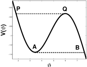
Figure 2: Wannier-Stark potential for $a=0.2$ and $k=0.7$.

This Hamiltonian is formally the Wannier-Stark Hamiltonian and stable islands are associated with elliptic motion near the bottom of the potential wells (Fig.2). A WKB estimate for the smallest decay rate from a well is

$$\Gamma\sim\frac{\omega_{0}}{2\pi}\;e^{-2S(A,B)/\hbar}$$ (3)

where $\omega_{0}$ is the angular frequency of the small oscillations and $iS(A,B)$ is the imaginary action along the classically forbidden path from point $A$ to point $B$, at constant energy equal to the value of the potential at the bottom of the well:

$$S(A,B)=\int_{\theta_{A}}^{\theta_{B}}d\theta\;\sqrt{2\epsilon(V(\theta)-V(\theta_{A}))}\;.$$

Reflection $\theta\to\pi-\theta$ turns $\theta_{A}$ into $\theta_{Q}$, $\theta_{B}$ into $\theta_{P}$, and reverses the sign of the argument of the square root; and so $S(A,B)=S(P,Q)$, the real action along the path from $P$ to $Q$ at constant energy equal to the value of the potential in $Q$. This path is the separatrix, so $2S(A,B)$ is equal to the area enclosed by the separatrix, which is in turn nearly equal to the area $\cal A$ of the actual island in the regime we are considering. Therefore,

$$\Gamma\sim\frac{\omega_{0}}{2\pi}e^{-{\cal A}/\hbar}.$$ (4)

This result is compared with a numerical simulation in Fig.3. Even better agreement with numerical data is obtained by using in (3) the trajectory with energy $\hbar\omega_{0}/2$ above the bottom of the well, which is an approximation to the ground state energy in the harmonic approximation. This is shown in Figs.3 and 4.
The success of the elementary WKB approximation (3) is due to the fact that in cases like Figs.3 and 4 the potential barriers on the right of $\vartheta_{B}$ are significantly lower than $V(\vartheta_{A})$, so that tunneling trajectories have to cross just one potential barrier. When this condition is not satisfied, one is faced with the full complexity of the WS problem.

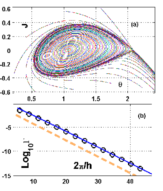
Figure 3: (Color online).(a) Phase portrait of system (1) with negative sign, for $\tilde{k}=0.8$ and $2\pi\Omega=0.7$. (b) Circles: numerically computed decay rate from the center of the regular island, as a function of $1/\hbar$. Lines show WKB estimates, obtained by using classically forbidden paths at constant energy (2). These are equal either to a minimum of the WS potential (dashed line) shown in Fig.2, or to the ground state energy in the potential well, estimated in the harmonic approximation (solid line).

III.2 Phenomenological Quantum Hamiltonian.

In Fig.4(b) we show the dependence of $\Gamma$ vs $\hbar$, for the case of the island of Fig.4(a). Like in the case of Fig.3, 2nd order resonances are not quite pronounced here, and so, at relatively large values of $\hbar$ (leftmost part of the Figure) the dominant contribution to decay is given by WS tunneling, and good agreement is observed with the theory of sect.III.1.

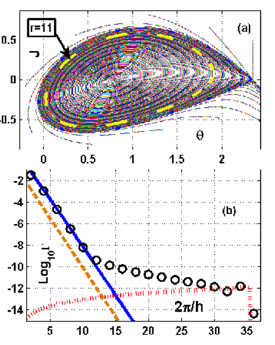
Figure 4: (Color online).Same as Fig.3 for $\tilde{k}=0.7$ and $2\pi\Omega=0.5$. The island chain highlighted in (a) is generated by a $11:1$ resonance at ${\mathcal{I}}_{111}\approx 0.251$, with $v=4.376\cdot 10^{-8}$, and $M=2.785$ (see App. B). The dotted line in (b) represents the theory (16) for decay assisted by this resonance, using the unperturbed spectrum (10).

As $\hbar$ decreases, a clear crossover is observed to slower decrease of $\Gamma$, indicating that a different mechanism of decay is coming into play, which overrules WS tunneling. In our interpretation, this is the mechanism of ”resonance assisted tunneling” to be discussed in what follows, which was introduced in ref.BSU02 . It is a quantum manifestation of classical KAM structures, and so we now consider the case when $\hbar$ is small compared to the size of the island, yet phase-space structures produced by higher-order corrections to the resonant Hamiltonian are not small on the scale of $\hbar$. The approach to be presently described is based on a quantum Hamiltonian, which is not formally derived from the exact dynamics, but is instead tailored after the actual structure of the classical phase space. This heuristic approach is applicable when the WS linewidth (4) is negligible with respect to the coupling between different WS tori (and between WS tori and the continuum) which is due to higher order corrections, and in fact it totally misses WS tunneling given by (4). It is assumed that the classical partition island/chaotic sea is quantally mirrored by a splitting of the Hilbert space of the system in a ”regular” and a ”chaotic” subspace, with respective projectors ${\hat{P}}_{r}$ and ${\hat{P}}_{c}$; and that the Hamiltonian ${\hat{H}}$ may be written as

$${\hat{H}}\; = \;{\hat{H}}_{r}\;+\;{\hat{H}}_{c}\;+\;{\hat{V}}\;+\;{\hat{V}}^{\dagger}\;,$$ (5)

where ${\hat{H}}_{r}={\hat{P}}_{r}{\hat{H}}{\hat{P}}_{r}$ is a ”regular” Hamiltonian, ${\hat{H}}_{c}={\hat{P}}_{c}{\hat{H}}{\hat{P}}_{c}$ is a ”chaotic” Hamiltonian, and ${\hat{V}}={\hat{P}}_{r}{\hat{H}}{\hat{P}}_{c}$ couples regular and chaotic states. In the case of maps, the Hamiltonian formalism has to be recovered by means of Floquet theory. Eigenvalues of Floquet Hamiltonians fall in Floquet zones, and for a system driven with a period $T$ in time, the width of a zone is $2\pi\hbar/T$. In our case we assume $T=1$ and so we identify the 1st Floquet zone with the interval $[0,2\pi\hbar)$. For the Hamiltonian ${\hat{H}}_{c}$ we assume in our case (where $a\neq 0$ is always understood) a continuous spectrum As this Hamiltonian is assumed to be ”chaotic”, we further assume that its quasi-energies are non-degenerate and completely fill each Floquet zone, because typical random matrices drawn from circular ensembles have simple spectra, with eigenphases uniformly distributed in $[0,2\pi]$. The discrete eigenvalues $E_{n}$ of the regular Hamiltonian ${\hat{H}}_{r}$ are therefore immersed in the continuous spectrum of the chaotic Hamiltonian ${\hat{H}}_{c}$, so the coupling perturbation ${\hat{V}}$ drives them off the real axis, and the imaginary parts $-i\hbar\Gamma_{n}/2$ they acquire are estimated by Fermi’s Golden Rule :

$$\Gamma_{n}\; \sim \;\frac{2\pi}{\hbar}|\langle E,c|{\hat{V}}^{\dagger}|E_{n}\rangle|_{E=E_{n}}^{2}\;.$$ (6)

where $|E,c\rangle$ is the eigenvector of ${\hat{H}}_{c}$ associated with an eigenvalue $E$ in the continuous spectrum ($\delta-$function normalization in energy is assumed for such eigenvectors). Choosing $E_{n}$ in the 1st Floquet zone of ${\hat{H}}_{c}$, (6) may be rewritten as

$$\Gamma_{n}\;\sim\frac{2\pi}{\hbar}\|{\hat{P}}_{0}{\hat{V}}^{\dagger}|E_{n}\rangle\|^{2}\mu(E_{n})\;.$$

where ${\hat{P}}_{0}$ is projection onto the 1st zone of ${\hat{H}}_{c}$. The function $\mu(E)$ is the Local Density of States, normalized to $1$, of the vector ${\hat{P}}_{0}{\hat{V}}^{\dagger}|E_{n}\rangle$ with respect to the chaotic Hamiltonian ${\hat{H}}_{c}$. It yields the probability that a transition prompted by ${\hat{V}}^{\dagger}$ from state $|E_{n}\rangle$ will lead to the continuum state $|E,c\rangle$ in the 1st zone. One may introduce the ”ergodic” assumption, that all in-zone transitions have the same probability. Then

$$\Gamma_{n}\;\sim\;\frac{1}{\hbar^{2}}\|{\hat{P}}_{0}{\hat{V}}^{\dagger}|E_{n}\rangle\|^{2}\;.$$ (7)

Whether or not the ergodic assumption is accepted, (7) may be assumed to hold up to a factor of order $1$.

III.3 Resonance-assisted decay.

At 1st order in $\epsilon$, the Hamiltonian ${\hat{H}}_{r}$ should correspond to the classical resonant Hamiltonian, and its eigenstates to quantized tori thereof. Therefore, the coupling ${\hat{V}}$ only reflects classical corrections of higher order than 1st, because the resonant Hamiltonian has no coupling between the inside and the outside of an island. Higher order corrections are present in ${\hat{H}}_{r}$ as well, and adding their secular (averaged) parts to the resonant Hamiltonian a new Hamiltonian ${\overline{H}}_{\mbox{\tiny res}}$ is obtained, which is still completely integrable, and shares the action variable ${\mathcal{I}}$ of the integrable WS pendulum flow (inside the WS separatrix). Semiclassical quantization of ${\overline{H}}_{\mbox{\tiny res}}$ yields energy levels $e_{n}={\overline{H}}_{\mbox{\tiny res}}({\mathcal{I}}_{n})$ with quantized actions ${\mathcal{I}}_{n}=(n+1/2)\hbar$.
In the following, by ”perturbation” we mean what is left of higher-order corrections, after removing averages. Thus the ”unperturbed” quasi-energy eigenvalues of ${\hat{H}}_{r}$ are given by $e_{n}+2\pi N\hbar$ with $N$ any integer ( $2\pi\hbar$ is the width of a Floquet zone). In the classical case, the destabilizing effects of the perturbation are mainly due to nonlinear resonances. A classical $r:s$ ($r,s$ integers) resonance occurs at ${{\mathcal{I}}}={{\mathcal{I}}}_{rs}$ if $r\omega({{\mathcal{I}}}_{rs})=2\pi s$, where $\omega({{\mathcal{I}}})=\partial{\overline{H}}_{\mbox{\tiny res}}({{\mathcal{I}}})/\partial{{\mathcal{I}}}$ is the angular frequency of the integrable motion in the island. The quantum fingerprints of classical nonlinear resonances are quasi-degeneracies in the quasi-energy spectrum. A degeneracy appears in the unperturbed quasi-energy spectrum of ${\hat{H}}_{r}$, anytime two or more energy levels $e_{n},e_{m},...$ are spaced by multiples of $2\pi\hbar$, that is the width of a Floquet zone. In the vicinity of a classical resonance ${\mathcal{I}}_{rs}$, this is approximately true, whenever $n-m$ is an integer multiple of $r$; for, in fact, $|e_{n}-e_{m}|\approx\hbar|n-m|\omega({\mathcal{I}}_{rs})=2\pi\hbar s|n-m|/r$. Thus, in the semiclassical regime, a classical resonance induces quantum quasi-degeneracies, which involve whole sequences of quantized tori. As such tori are strongly coupled by the perturbation, decay is enhanced. This quantum effect is Resonance Assisted Decay BSU02 .
The perturbative approach assumes that the sought for metastable states basically consist of superpositions of such strongly coupled, quasi-degenerate states. This leads to replacing ${\hat{P}}_{r}$ in (5) by projection ${\hat{P}}_{\mbox{\tiny R}}$ onto a quasi-degenerate subspace, similar to methods used in naama ; and so, in order to use Fermi’s rule (7), ${\hat{P}}_{\mbox{\tiny R}}{\hat{H}}{\hat{P}}_{\mbox{\tiny R}}$ must be diagonalized, and ${\hat{P}}_{\mbox{\tiny R}}{\hat{V}}$ must be specified. To this end we first write the matrix of ${\hat{P}}_{\mbox{\tiny R}}{\hat{H}}{\hat{P}}_{\mbox{\tiny R}}$ in a basis of quasi-degenerate states. Let ${{\mathcal{I}}}_{n_{0}}$ be a quantized action close to ${{\mathcal{I}}}_{rs}$. The energy levels $e_{n_{0}+Nr}$, where the integer $N$ takes both negative and positive values, have an approximately constant spacing, close to $2\pi\hbar s$, and thus form a ladder. There is one such ladder for each choice of the integer $n_{0}$ in the set of the $r$ closest integers to $n_{rs}\equiv{\mathcal{I}}_{rs}/\hbar-1/2$ (not necessarily an integer), and we fix one of them. The quasi-energy levels $e_{n_{0}+Nr}-2\pi\hbar Ns$ are quasi-degenerate . Denoting $|N\rangle$ the corresponding eigenstates, the projector ${\hat{P}}_{\mbox{\tiny R}}$ onto the ladder subspace is a finite sum $\sum_{N}|N\rangle\langle N|$, where $N$ ranges between a $N_{*}<0$ and a $N^{*}>0$. The number of terms in the sum is equal to the number of nearly resonant states inside the island and so is given by $L+1$ where $L=N^{*}-N_{*}$. Using that the actions ${I}_{N}$ of levels in a $r:s$ ladder are approximately spaced by multiples of $r\hbar$, $L$ is estimated by

$$L\;\approx\;\mbox{\rm Int}\left[\left(\frac{\cal A}{2\pi\hbar}-1\right)\frac{1}{r}\right]\;.$$ (8)

If only nearest-neighbor transitions are considered, the matrix of ${\hat{P}}_{\mbox{\tiny R}}{\hat{H}}{\hat{P}}_{\mbox{\tiny R}}$ over the basis $|N\rangle$ is tridiagonal, of size $L+1$. The off-diagonal elements $v(N)=\langle N|{\hat{H}}|N+1\rangle$ may be semiclassically assumed to slowly change with $N$, and will be hence denoted simply by $v$. The diagonal elements are the nearly degenerate quasi-energies $W(N)=e_{n_{0}+Nr}-Nsh$, and Taylor expansion of ${\overline{H}}_{\mbox{\tiny res}}({{\mathcal{I}}})$ to 2nd order near ${{\mathcal{I}}}_{rs}$ yields

$$W(N)\approx{\overline{H}}_{\mbox{\tiny res}}({\mathcal{I}}_{rs})+2\pi\hbar\frac{s}{r}(n_{0}-n_{rs})+\frac{\hbar^{2}}{2M}(n_{0}+rN-n_{rs})^{2}$$ (9)

where $M=1/\omega^{\prime}({{\mathcal{I}}}_{rs})$. It follows that, apart from a constant (independent on $N$) shift, the diagonal matrix elements of ${\hat{P}}_{\mbox{\tiny R}}{\hat{H}}{\hat{P}}_{\mbox{\tiny R}}$ are

$$W(N)\approx\frac{\hbar^{2}}{2M}(rN+\delta n)^{2}\;.$$ (10)

where $\delta n=n_{0}-n_{rs}$. Replacing this in ${\hat{P}}_{\mbox{\tiny R}}{\hat{H}}{\hat{P}}_{\mbox{\tiny R}}$, one easily recognizes that the classical limit $\hbar\to 0$, $L\to\infty$ of ${\hat{P}}_{\mbox{\tiny R}}{\hat{H}}{\hat{P}}_{\mbox{\tiny R}}$ is the classical pendulum Hamiltonian:

$${\cal H}_{rs}({\mathcal{I}}^{*},\theta^{*})=\frac{r^{2}{\mathcal{I}}^{*2}}{2M}+2v\cos(\theta^{*})\;,$$ (11)

in appropriate canonical variables ${\mathcal{I}}^{*},\theta^{*}$ ($N\hbar\sim{\mathcal{I}}^{*}=({\mathcal{I}}-{\mathcal{I}}_{rs})/r$ as $\hbar\to 0$). This is the well-known pendulum approximation near a classical resonance LL92 , directly derived from quantum dynamics ZA , and is related by a simple canonical transformation to the slightly different Hamiltonian (22) which is used in BSU02 .
The coupling to continuum ${\hat{P}}_{\mbox{\tiny R}}{\hat{V}}$ remains to be specified. Of all quantized tori in the chain, the closest to the chaotic sea corresponds to state $|N^{*}\rangle$, and we assume that this one state (in the given chain) is coupled to the continuum. This assumption implies :

$${\hat{V}}^{\dagger}{\hat{P}}_{\mbox{\tiny R}}\;=\;|\chi\rangle\langle N^{*}|\;,$$ (12)

where $|\chi\rangle$ is some vector in the chaotic subspace, about which our one assumption is that it lies in the 1st Floquet zone. Its norm has the meaning of a hopping amplitude from the ”gateway state” $|N^{*}\rangle$ to the normalized state $||\chi||^{-1}|\chi\rangle$. The latter state may be thought of as a ”last beyond the last” nearly resonant state, corresponding to an unperturbed torus which was sunk into the stochastic sea by the perturbation and so cannot any more support a regular quasi-mode of ${\hat{H}}_{r}$. Thus one may denote $||\chi\rangle||=v(N^{*})$, and extrapolate to this last transition, too, the semiclassical assumption $v(N^{*})\sim v$. After all such additional constructions, the ”ergodic assumption” (end of section III.2) is just that this last state has equal projections on all eigenstates of ${\hat{H}}_{c}$. Fermi’s rule (7) now yields, for the decay from an eigenstate $|E_{m}\rangle$ $(0\leq k\leq L)$ of ${\hat{P}}_{\mbox{\tiny R}}{\hat{H}}{\hat{P}}_{\mbox{\tiny R}}$,

$$\Gamma_{m}\sim\frac{v^{2}}{\hbar^{2}}|\langle N^{*}|E_{m}\rangle|^{2}\;.$$ (13)

The labeling $m=0,\ldots,L$ of the eigenstates of ${\hat{P}}_{\mbox{\tiny R}}{\hat{H}}{\hat{P}}_{\mbox{\tiny R}}$ is arbitrary for the time being. The tridiagonal Hamiltonian is defined on a chain of states and the scalar product in the last formula is the value of the eigenfunction $\langle N|E_{m}\rangle$ at the rightmost site $N=N^{*}$ in the chain. Assuming the eigenfunction to attain its maximum modulus at a site $N_{m}$, its value at site $N^{*}$ should be of order $\exp(-\xi_{m}|N^{*}-N_{m}|)$. The quantity $\xi_{m}^{-1}$ is the fall-off distance of this eigenfunction. For a tridiagonal Hamiltonian on a chain, arguments by Herbert, Jones, and Thouless Thou72 , estimate this distance , as

$$\xi_{m}\sim\ln\left(\frac{{D_{m}}}{\overline{v}}\right)\;,$$ (14)

where ${{D_{m}}}$ is the geometric average of the differences $|E_{j}-E_{m}|$ ($m$ fixed, $j$ variable, $j\neq m$), that is

$$\ln({{D_{m}}})=\frac{1}{L}\sum\limits_{j(\neq m)=0}^{L}\ln(|E_{j}-E_{m}|)\;,$$ (15)

and $\overline{v}$ is the geometric average of the hopping coefficients $v(N)$, ($N_{*}\leq N\leq N^{*}-1$). Under the assumption $v(N)\approx v=$const., ${\overline{v}}=v$, and so finally

$$\Gamma_{m}\;\sim\;\frac{v^{2}}{\hbar^{2}}\left(\frac{v}{{{D_{m}}}}\right)^{2(N^{*}-N_{m})}\;.$$ (16)

It should be emphasized that the $E_{m}$ used in (15) are the eigenvalues of ${\hat{P}}_{\mbox{\tiny R}}{\hat{H}}{\hat{P}}_{\mbox{\tiny R}}$ and not its diagonal elements $W_{m}$ (10), and that eqn. (14) is not perturbative.

III.4 Single-Resonance Assisted Decay.

At any $v\neq 0$, an island hosts a dense set of resonances, but only a few of them are quantally resolved. On the other hand, quasi-resonant ladders of states may be formed, only if the resonant transitions are not so broad as to involve off-ladder states. That means that the classical chain of islands should not be too wide, because its width is determined by the same parameter $v$ which yields the hopping amplitude between nearly resonant states.
In this section we consider the case when a single, not too wide resonance dominates all the others, so that each metastable state may be assumed to sit on one of the ladders which are associated with that resonance. Decay rates $\Gamma_{m}$ are not affixed to unperturbed tori, but to eigenstates $|E_{m}\rangle$ of a ladder Hamiltonian. For $v=0$ these correspond to quantized tori in the quasi-resonant ladder, via (10), and their labeling by $m=0,\ldots,L$ may be chosen accordingly. For not quite small $v$, however, the correspondence between metastable states and unperturbed tori may be broken, due to avoided crossings; and so labeling by the original quantum number may not anymore reflect how deep in the island an eigenstate is located.
We restrict the following discussion to decay ”from the center of the island”, meaning that we consider a metastable state, which is mostly supported in the innermost part of the island, and is labeled by $m=0$. For this state, (16) reads:

$$\Gamma_{0}\;\sim\;\frac{v^{2(L+1)}}{\hbar^{2}D_{0}^{2L}}\;=\;\frac{v^{2}}{\hbar^{2}}e^{-2\xi_{0}L}\;\;\;;\;\;\;\xi_{0}=\ln(D_{0})-\ln({v}).$$ (17)

For quite small $v$, explicit calculation is possible, using for $E_{j}$ their unperturbed ($v=0$) values given by (10). This leads to

$$|E_{j}-E_{0}|\approx\hbar^{2}|r^{2}j^{2}-2n_{rs}rj|/2M,$$ (18)

and then (16) with (14) and (15) leads to

$$\xi_{0}\simeq\ln\left(\frac{\hbar^{2}}{2Mv}\right)+\frac{1}{L}\sum\limits_{j=1}^{L}\ln(|r^{2}j^{2}-2n_{rs}rj|)\;.$$ (19)

to be used in (17). In the average, (17) takes the form (cp.(8)):

$$\Gamma_{0}\sim\frac{v^{2}}{\hbar^{2}}e^{-\xi_{0}{\cal A}/\pi r\hbar}\;,\;.$$ (20)

This equation shows that the average dependence of $\Gamma_{0}$ on $1/\hbar$ is exponential, because the dependence of $\xi_{0}$ on $\hbar$ is semiclassically weak. In fact, $v$ is a classical quantity, and in the limit $\hbar\to 0$ the average over levels $E_{j}$ which enters eqn. (15) turns into a purely classical quantity, given by the phase-space average of $\ln({\cal H}_{rs}-E_{0})$ (cp.(11)) over the island.

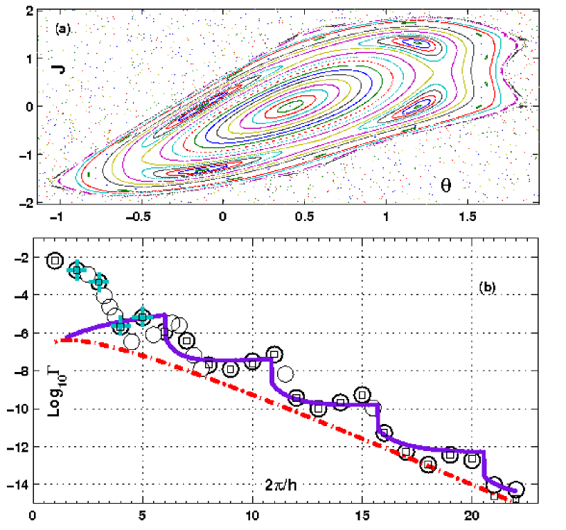
Figure 5: (Color online).(a) Phase portrait of map (1) with negative sign, for ${\tilde{k}}=2.5$ and $2\pi\Omega=1$. The 4-islands chain is due to a $4:1$ resonance at ${\mathcal{I}}_{41}\approx 0.43$, with $v\approx 7.275.10^{-4}$ and $M\approx 3.866$. (b) Minimal decay rate from the island shown in (a), calculated by different numerical (symbols) and theoretical (lines) methods. Circles: truncated basis method. Pluses: long-time decay of an initial coherent state in the center of the island. Small Squares : Complex Scaling Method. Solid line : formula (17), with (19). Dotted-dashed line: continuum approximation (20),(21).

Approximating the sum in (19) by an integral, and denoting ${\cal A}_{rs}=2\pi{{\mathcal{I}}}_{rs}=2\pi\hbar n_{rs}$ the area enclosed by the $r:s$ resonant unperturbed torus, and $x={\cal A}_{rs}/{\cal A}$,

$$\xi_{0}\sim-\ln\left(\frac{8\pi^{2}Mv}{{\cal A}^{2}}\right)-2+2x\ln(2x)+(1-2x)\ln(|1-2x|)\;\;.$$ (21)

In formula (17) (with (19)), $L$ is anyway a discrete variable, which discontinuously jumps by $1$ anytime increase of $1/\hbar$ grants accommodation of a new quasi-resonant torus in the island (cp.(8)). This produces a stepwise dependence of $\Gamma_{0}$ on $1/\hbar$, superimposed on the average exponential dependence. This structure is smoothed in (20) with (21).

III.5 Numerical results for resonance assisted decay.

Eqns.(17) and (20) (supplemented by (19) or (21)) are the main results of the theory of resonance assisted decay and are tested against numerical results in this section. They require specification of $M,v,{\mathcal{I}}_{rs}$ as input parameters. In the case of well-pronounced chains of resonant islands, the values of $M,v$, and ${\mathcal{I}}_{rs}$ may be found by ”measuring” areas in the classical phase-space portrait, taking advantage of the fact that a resonant chain is bounded in between the separatrices of a pendulum (11). This method was introduced in BSU02 , and is reviewed in Appendix B for the reader’s convenience.
For small $v$, unperturbed eigenvalues (10) may be used in (15) for the purpose of calculating $D_{m}$, leading to (17) (with (19)), but one has to beware of values of $\hbar$, that enforce degeneracy of the unperturbed spectrum (10). Inadvertent use of the spectrum (10) in (15) in such cases leads to artificial divergence of $\Gamma$. In the actual spectrum to be used in (15), degeneracies are replaced by avoided crossings, which may lead to local enhancement of resonance-assisted tunneling, as discussed in Appendix C and shown in Fig. 11.
A case with a single dominant resonance $4:1$ is presented in Fig.5 . Decay rates calculated from (17) with (10) and (19) are shown in (b) for the innermost state in the island which is shown in Fig.5(a). Also shown are results of directly calculating $\Gamma$s, by methods described in Appendix A. Formula (17), with (19), is seen to correctly reproduce the actual $\Gamma$s, in order of magnitude at least. The stepwise dependence predicted in BSU02 and explained in the end of previous section is here remarkably evident. The continuum (quasiclassical) approximation (20),(21) is also shown in the same Figure. In Fig.6 it is seen to better and better agree with (17), with (19), at smaller and smaller values of $\hbar$.

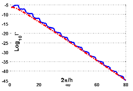
Figure 6: (Color online).Comparison between (17), with (19), and the continuum formula (20),(21)

As remarked in section III.4, the presented theory, being essentially perturbative, is expected to fail in the case of large classical resonances. An example is presented in Fig.7.

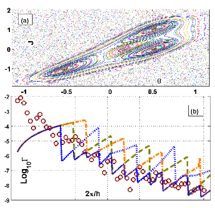
Figure 7: (Color online).Illustrating a case with a very broad resonant chain. (a): Phase portrait of Map(1) with negative sign, for ${\tilde{k}}=\pi$ and $2\pi\Omega=0.5$. The numerical values for the $3:1$ resonance are $I_{31}=0.13,v=1.9\cdot 10^{-3},M=1.52$ (b): Minimal decay rate from the island, vs $2\pi/\hbar$. Circles: numerical data (truncated basis). Dotted, dashed, and dash-dotted lines show decay rates for the three lowest-lying states in the island, computed from the theory of decay assisted by the large $3:1$ resonance . The solid line shows the smallest of these.

Finally in Fig.8 we present a case with two resonant chains of comparable size. Results are not well described by the theory based on either resonance, and thus appear to contradict a somewhat natural expectation, that each resonance should contribute its own set of metastable states. The single-ladder picture may not be adequate in such cases, which therefore remain outside the present scope of the theory.

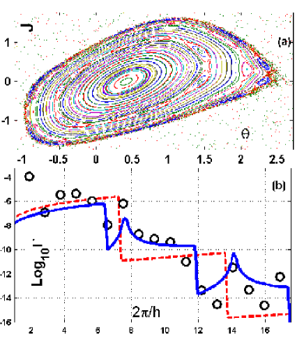
Figure 8: (Color online).Illustrating a case with two classical resonances of comparable size. Here ${\tilde{k}}=1.329$ and $2\pi\Omega=0.5336$. Circles in (b) represent the minimal decay rates from the truncated basis method. Lines in (b) represent the theory of Resonance Assisted decay, using either the $6:1$ resonance (solid line) or the $7:1$ resonance (dashed line). The former resonance has $v=1.8\cdot 10^{-4},M=4.504,{\mathcal{I}}_{61}=0.46$, and the latter has $v=3.1\cdot 10^{-4},M=2.626,{\mathcal{I}}_{71}=0.93$.

IV Discussion and Conclusions

The decay rates of some metastable states related to phase space islands were calculated and the required theoretical framework was developed. The main results of the paper are (4), (16) and (17), where the decay rates of wave packets in phase space islands were calculated for various conditions. If the effective Planck’s constant is sufficiently large, so that island chains cannot be resolved on its scale, standard WKB theory was found to work well. As the effective Planck’s constant is decreased, island chains are resolved, and dominate the decay by the mechanism of resonance assisted tunneling. Its signature here is the step structure of Fig.5(b). The average slope of $\ln\Gamma$ (see (20)) as a function of $1/\hbar$ is $-\xi_{0}{\cal A}/\pi r$, with $\xi_{0}$ given by (21) and is independent of $\hbar$. In the WKB regime a different slope is found (see (4)). For some values of the parameters, resonance-assisted tunneling can be further enhanced by a degeneracy between a semiclassical state deep inside the island and one that is close to the boundary. An interesting question is about possible effects of this kind, due to ”vague tori” SR82 , i.e., to classical structures which quantally act as tori, in spite of lying outside an island. Indeed, observations in FGR00 have suggested a possible role for cantori in enhancing QAMs at times.
The theory strongly relies on the dominance of one resonant island chain If the phase space area of the chain is not small as is the case in Fig.7 or if the tunneling is assisted by two (or more) resonant island chains of approximately equal strength, as is the case in Fig.8, our theory requires modification.

The theory is relevant for systems of experimental interest but the steps of Fig.5 were found for a regime where the decay rate is too small to be experimentally accessible. Overcoming this problem is a great theoretical and experimental challenge.

Appendix A Metastable states.

Our methods of computing decay rates $\Gamma$ were: (1) basis truncation, (2) complex scaling, (3) simulation of wave-packet dynamics. In the cases investigated in this paper, the most economical one, and thus the one of our prevalent use, was (1). The other two methods were used to cross-check results of (1) in a number of cases. The observed agreement between such completely independent computational schemes demonstrates the existence of resonances (in the sense of metastable states).

A.1 Basis Truncation.

Let ${\hat{U}}$ denote the unitary evolution operator that is obtained by quantizing map (1), as described in sect.II.2; and let $|n\rangle$, $(n\in{\mathbb{Z}})$ be the eigenvectors of the angular momentum operator ${\hat{J}}$, such that $\langle\theta|n\rangle=(2\pi)^{-1/2}\exp(in\theta)$. ”Basis truncation” consists in replacing ${\hat{U}}$ by ${\hat{U}}_{\nu}={\hat{P}}_{\nu}{\hat{U}}{\hat{P}}_{\nu}$, where ${\hat{P}}_{\nu}=\sum_{|n|\leq\nu}|n\rangle\langle n|$. This introduces an artificial dissipation, which turns the quantum dynamics from unitary to sub-unitary. The eigenvalues $z_{j}$, $(j=1,\ldots,2\nu+1)$ of ${\hat{U}}_{\nu}$ lie inside the unit circle, with positive decay rates $\Gamma_{j}=\ln(1/|z_{j}|)/2$. As $\nu$ is increased, most of them move towards the unit circle, but some appear to stabilize at fixed locations inside the circle, because they approximate actual, subunitary eigenvalues of the exact $(\nu=\infty)$ non-dissipative dynamics. The seeming contradiction to unitarity of the limit dynamics ${\hat{U}}$ is solved by the observation that the eigenfunctions of ${\hat{U}}_{\nu}$, which are associated with such eigenvalues, tend to increase in the negative momentum direction (Fig.10), as expected of Gamov states, and if this behavior is extrapolated to the limit, then they cannot belong in the Hilbert space wherein ${\hat{U}}$ acts unitarily. In order to make room for such non-unimodular eigenvalues, ${\hat{U}}$ must be extended to a larger functional space. Complex scaling, to be described in the next subsection, provides a consistent method of doing that.
Simulations of wave packet dynamics, performed in the total absence of any dissipation whatsoever, confirm this interpretation of the stable subunitary eigenvalues (Fig.9). The initial wave packet is a coherent state supported near the center of the island . We use a FFT algorithm, so the computed evolution is fully unitary, and reliably reproduces the exact evolution over a long time, thanks to the large dimension of the FFT . We compute the decay in time of the probability in a momentum window which contains the classical island. After an initial rapid decay, due to escape of the part of the distribution which initially lies outside the island, the decay turns into a clean exponential with rate $\gamma\approx 5.66$ (Fig.10). Among the eigenfunctions of the truncated basis evolution, which correspond to stabilized eigenvalues, we select the one which has largest overlap with the chosen initial state. We thus find that (i) the decay rate $\Gamma$ of this eigenfunction is $\approx\gamma$, (ii) the Husimi function of that part of the wavepacket, which has survived in the chosen window until the end of the dynamical calculation, nearly reproduces the Husimi function of the eigenfunction (Fig.9).
Numerical computation of long-time exponential decay may be less easy than in the above particular example. If an initial state is overlapped by several metastable states with slightly different $\Gamma$, resolving them may take quite a long computational time, and hence a huge basis, because of accelerated motion outside the island.

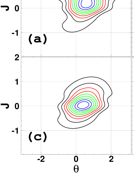
Figure 9: (Color online).(a),(b),(c): Evolution of an initial coherent state located at the center of the island of Fig.5, for ${\tilde{k}}=2.5$, $2\pi\Omega=1$, $\hbar=0.25$, numerically simulated by a FFT method with basis size $2^{17}$. (a),(b),(c) show contour plots of the Husimi functions at times t=100, t=1000, t=16000 respectively. (d): Husimi contour plot of the eigenfunction of the truncated basis dynamics, which has the largest overlap with the initial coherent state. The size of the truncated basis is $4096$.

A.2 Complex Scaling.

Scattering resonances may be sometimes computed by diagonalizing a non-hermitean Hamiltonian, which is constructed by ”complex coordinate” methods such as analytic dilation, and the like MSV03 ; RS78 . Despite absence of scattering theory, a method of this sort was devised for the subunitary eigenvalues considered in this paper, as follows. Any function $\psi(\theta)$ over $[0,2\pi]$ is at once a function $\tilde{\psi}(z)$ of the complex variable $z$ running on the unit circle. Let ${\cal B}$ denote the class of those functions $\psi(\theta)$, which can be analytically continued to the whole complex plane, except possibly the origin. For given $1\geq\rho>0$ the scaling operator $h_{\rho}$ is defined to act on the functions of this class as in $(h_{\rho}\psi)(\theta)=\tilde{\psi}(\rho e^{i\theta})$. The crucial property of the operator ${\hat{U}}$, which makes the present construction possible, is that of transforming functions in class ${\cal B}$ in functions in the same class, and so the operator $U_{\rho}\equiv h_{\rho}{\hat{U}}h^{-1}_{\rho}$ is a well defined operator in ${\cal B}$. This operator trivially extends by continuity to an operator $U_{\rho}$ G06 which is defined on the whole of $L^{2}([0,2\pi])$. This extension formally amounts to defining ${\hat{U}}$ also on a class of functions, which are not square integrable. The new “functions” thus acquired in the domain of the evolution operator may be very singular objects; e.g., in the momentum representation, they are allowed to exponentially diverge at infinity. In the special case $\hbar=1/n$ with $n$ integer, ${\hat{U}}_{\rho}$ has the form :

$${\hat{U}}_{\rho}=\rho^{n}e^{i{n\hat{\theta}}}e^{-ik_{+}\cos({\hat{\theta}})}e^{k_{-}\sin({\hat{\theta}})}e^{-i{\hat{J}}^{2}/2}\;\;,\;k_{\pm}=\frac{1}{2}{\tilde{k}}\left|\rho\pm\rho^{-1}\right|\;.$$

which restitutes ${\hat{U}}$ for $\rho=1$. The eigenvalues of ${\hat{U}}_{\rho}$ as a $L^{2}$ operator are at once eigenvalues of the “extended” ${\hat{U}}$, and each of the latter eigenvalues is an eigenvalue of ${\hat{U}}_{\rho}$ for $\rho$ sufficiently distant from $1$. The ”complex scaling” method of computing $\Gamma$, which is mentioned in the main text, consists in diagonalization of ${\hat{U}}_{\rho}$. At small $\hbar$ this method is computationally problematic, due to exponentially large elements in the matrix of ${\hat{U}}_{\rho}$.

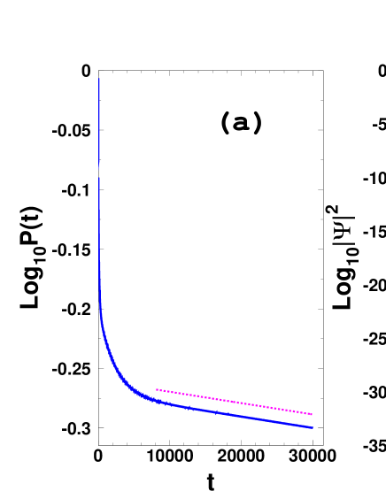
Figure 10: (Color online).(a): Decay in time of the probability in a momentum window containing the island, for the same parameter values as in Fig.9, and for the same choice of the initial state. The size of the basis used in the simulation is $2^{18}$. The straight line has slope $\approx-5.66$. (b) squared modulus of the truncated basis eigenfunction presented in Fig.9(d), in the momentum representation.

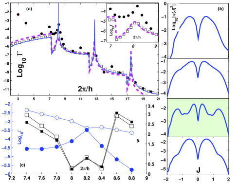
Figure 11: (Color online).(a) Decay rate from the 1st excited state in the island, vs $1/\hbar$, for the same parameter values as in Fig.5. Dots: numerical (truncated basis method). Solid line: formula (16) with (15), using the unperturbed ladder spectrum (10). Squares: same formula, using the perturbed spectrum of the tridiagonal matrix with (10) as diagonal elements. Dashed line: same formula, using the actual spectrum, semiclassically reconstructed from the layout of tori in the island. (b) the eigenstate of the (truncated) evolution operator, corresponding to the decay rate shown in (a) for values of $1/\hbar$: $7$, $8$, $8.2$ and $8.6$ (from above down), in the momentum $J$ representation. Only a $J-$interval of roughly the size of the island is shown. (c) Decay rate $\Gamma$ (circles) and real quasi-energy $w$ (squares) vs $1/\hbar$, for the 1st (full symbols) and the 5th (empty symbols) excited states.

Appendix B Inferring Parameters of a Classical Resonance from Phase Portraits.

Parameters ${\mathcal{I}}_{rs}$, $M$, and $v$ of a classical $r:s$ resonance respectively specify the value of the unperturbed action where the resonance is located, the inverse nonlinearity $1/\omega^{\prime}({\mathcal{I}}_{rs})$, and the strength of the resonant harmonic perturbation. These parameters are indispensable for the formalism described in sect.III.3, and may be retrieved from the phase-space portrait, using formulae taken from ES05 . Here we reproduce a sketchy derivation for the reader’s convenience. Motion in a $r:s$ resonant chain is approximately described by a pendulum Hamiltonian LL92 , which may be written in the form (which is canonically equivalent to (11):

$$H_{rs}({{\mathcal{I}}},\varphi)=\frac{1}{2M}({\mathcal{I}}-{\mathcal{I}}_{rs})^{2}\;+\;2v\;\cos(r\varphi)\;.$$ (22)

In this paper, ${\mathcal{I}}$ is the action variable of the WS-pendulum Hamiltonian (2). The Separatrices of Hamiltonian (22) are the curves ${\mathcal{I}}={\mathcal{I}}_{\pm}(\varphi)={\mathcal{I}}_{rs}\pm 2\sqrt{Mv(1-\cos(r\varphi))}$, and so the phase areas $S_{\pm}$ they enclose satisfy:

$$S_{+}\;+\;S_{-}\; = \;4\pi{\mathcal{I}}_{rs}\;,$$

$$S_{+}\;-\;S_{-}\; = 2\int_{0}^{2\pi}d\varphi\;({\mathcal{I}}_{+}(\varphi)-{\mathcal{I}}_{rs})\;=\;16\sqrt{2Mv}\;.$$ (23)

The monodromy matrix of the stable period-$r$ orbit that is responsible for the resonant chain is easily obtained by linearizing the flow (22) near the stable equilibrium point(s). Its trace is found to be ${\cal M}=2\cos(r\nu)$ where $\nu=r\sqrt{2v/M}$ is the angular frequency of the small pendulum oscillations. This leads to

$$\sqrt{2v/M}\;=\;r^{-2}\arccos({\cal M}/2)\;.$$ (24)

The phase-space areas $S_{\pm}$ and the Monodromy Matrix can be numerically determined, and once their values are known eqs.(B) and (24) can be solved for ${\mathcal{I}}_{rs}$, $M$, and $v$.

Appendix C Avoided Crossings.

An exact degeneracy arises in the unperturbed ladder spectrum (10) whenever two quantized actions in the ladder are symmetrically located with respect to the the resonant action ${\mathcal{I}}_{rs}$. This requires $\delta n=0$ or $\delta n=\pm r/2$ in (10) and so, if $(n_{i}+1/2)\hbar$ is the smallest quantized action in the ladder, such symmetric pairs exist if, and only if,

$$\frac{1}{\hbar}=\frac{2n_{i}+lr+1}{2{\mathcal{I}}_{rs}}\;\;\mbox{\rm and}\;\;L(\hbar)\geq l\;,$$ (25)

for some integer $l\geq 1$. In the above inequality, the length $L$ of the ladder depends on $\hbar$ as in (8). In the case of Fig.5, where $n_{i}=0$ (the ground state), (25) is never satisfied for $1/\hbar<20$. The data in Fig.5 were computed using the spectrum (10), and no significant difference could be found between them and data computed by using the actual spectrum, semiclassically reconstructed from the layout of tori in the island. In Fig.11, where $n_{i}=1$ (the ”1st excited state”), (25) is satisfied for $1/\hbar=8.2,12.8,17.44$, corresponding to $l=1,2,3$. At such values of $1/\hbar$ the spectrum (10)(with the appropriate $\delta n$) is degenerate and using it in formulas (15),(16) obviously causes $\Gamma$ to diverge, as shown by the narrow peaks in Fig.11. Such artifacts disappear on inserting the proper (perturbed) spectrum, obtained by diagonalizing the ladder Hamiltonian with the diagonal elements given by (10), because for $v\neq 0$ the spectrum is never degenerate. Nevertheless avoided crossings take place at the values (25) of $\hbar$, giving rise to local peaks in the dependence of $\Gamma$ on $\hbar$.
At the same values of $1/\hbar$ avoided crossings are observed even between subunitary, stabilized eigenvalues of the truncated evolution operators (see App.A). This is shown in Fig.11(c). The eigenvalues are written $z=e^{-\Gamma/2-iw}$ and it is seen that, as $1/\hbar$ approaches a value $\approx 8.2$, a pair of complex eigenvalues undergo a close avoided crossing. The corresponding states exhibit standard behavior at avoided crossings. The distribution in momentum $J$ of one of them is shown in Fig.11). This state nominally corresponds to the $n=1$ unperturbed state, and in fact in (b)(top) it looks similar to the 1st excited state of a harmonic oscillator. The other state nominally corresponds to the $n=5$ unperturbed state. At the avoided crossing (3d inset from top in (b)) the former state significantly expands over the island, because it is basically a superposition of two unperturbed states, which are located symmetrically with respect to ${\mathcal{I}}_{41}$. This gives rise to a local enhancement of the decay rate.

References

- (1) A.J.Lichtenberg and A.A.Lieberman, Regular and Chaotic Motion, Springer-Verlag NY, (1992).
- (2) J. U. N ckel and A. D. Stone, Nature 385 (London), 45 (1997); C. Gmachl, F. Capasso, E. E. Narimanov, J. U. N ckel, A. D. Stone, J. Faist, D. L. Sivco, and A. Y. Cho, Science 280, 1556 (1998); H. E.Tureci, H. G. L. Schwefel, A. D. Stone, and E. E. Narimanov, Opt. Express 10, 752 (2002).
- (3) W. K. Hensinger, H. Haffner, A. Browaeys, N. R. Heckenberg, K. Helmerson, C. McKenzie, G. J. Milburn, W. D. Phillips, S. L. Rolston, H. Rubinsztein-Dunlop, and B. Upcroft, Nature 412 (London), 52 (2001); D. A. Steck, W. H. Oskay, and M. G. Raizen, Science 293, 274 (2001).
- (4) V. Averbukh, S. Osovski, and N. Moiseyev, Phys. Rev. Lett. 89, 253201 (2002); S. Osovski, and N. Moiseyev, Phys. Rev. A 72, 033603 (2005).
- (5) D. Turaev and V. Rom-Kedar, Nonlinearity 11, 575 (1998); V. Rom-Kedar and D. Turaev, Physica D 130, 187 (1999).
- (6) A. Kaplan, N. Friedman, M. F. Andersen, and N. Davidson, Phys. Rev. Lett. 87, 274101 (2001); M. F. Andersen, A. Kaplan, N. Friedman, and N. Davidson, J. Phys. B: At. Mol. Opt. 35, 2183 (2002); A. Kaplan, N. Friedman, M. F. Andersen, and N. Davidson, Physica D 187, 136 (2004).
- (7) O. Bohigas, S. Tomsovic and D. Ullmo, Phys. Rep. 223, 43 (1993); S. Tomsovic and D. Ullmo, Phys. Rev. E 50, 145 (1994); F. Leyvraz and D. Ullmo, J. Phys. A 29, 2529 (1996); E. Doron and S. D. Frischat, Phys. Rev. Lett. 75, 3661 (1995); S. D. Frischat and E. Doron, Phys. Rev. E 57, 1421 (1998); J. Zakrzewski, D. Delande and A. Buchleitner, Phys. Rev. E 57, 1458 (1998).
- (8) A. Iomin, S. Fishman and G.M. Zaslavsky, Phys. Rev. E 65, 036215 (2002); J.D. Hanson, E. Ott and T.M. Antonsen, Phys. Rev. A 29, 819 (1984).
- (9) O.Brodier, P.Schlagheck and D.Ullmo, Ann. Phys. 300 (2002) 88.
- (10) V.A.Podolsky and E.E.Narimanov, Phys. Rev. Lett. 91, 263601 (2002).
- (11) C.Eltschka and P.Schlagheck, Phys. Rev. Lett. 94, 01401 (2005).
- (12) A.Bäcker, R.Ketzmerick, A.Monastra, Phys. Rev. Lett. 94, 054102, (2005).
- (13) M.K.Oberthaler, R.M.Godun, M.B.d’Arcy, G.S.Summy and K.Burnett, Phys. Rev. Lett. 83,4447, (1999); R.M.Godun, M.B.d’Arcy, M.K.Oberthaler, G.S.Summy, and K.Burnett, Phys. Rev. A62, 013411, (2000).
- (14) S.Fishman, I.Guarneri, L.Rebuzzini, Phys. Rev. Lett. 89, 084101, (2002); J.Stat.Phys. 110, 911, (2003).
- (15) M.B. d’Arcy, G.S. Summy, S. Fishman and I. Guarneri, Physica Scripta 69, C25-31, (2004).
- (16) I.Guarneri, L.Rebuzzini and S.Fishman, preprint, (2005).
- (17) M.Glück, A.R.Kolovsky, and H.J.Korsch, Phys. Rep. 366, 103, (2002).
- (18) M.Glück, A.R. Kolovsky, H.J.Korsch, N.Moiseyev, Eur. Phys. J. D4,239, (1998).
- (19) D.Boyanovsky, R.Wiley, R.Holman, Nucl. Phys. B 376,599, (1992).
- (20) L.Schulman, Techniques and Applications of Path Integration, Wiley-Interscience, (1996), ch. 29.
- (21) D.J.Thouless, J.Phys. C: Solid State Phys. 5, 77, (1972); D.C. Herbert and R. Jones, J.Phys. C: Solid State Phys. 4, 1145, (1971).
- (22) G.M. Zaslavsky, Phys. Rep. 80, 157, (1981).
- (23) N.Moiseyev, Phys. Rep. 302, 811, (1998).
- (24) M.Reed and B.Simon, Methods of Modern Mathematical Physics IV: Analysis of Operators, Academic Press, (1978).
- (25) I.Guarneri, unpublished (2005)
- (26) R.B. Shirts and W.P. Reinhardt, J. Chem. Phys. 77, 5204, (1982).
- (27) N.Brenner and S. Fishman, Phys. Rev. Lett. 77, 3763, (1996); N.Brenner and S. Fishman, J. Phys. A 28, 5973, (1995); C. de Oliveira, I.Guarneri and G.Casati, Europhys. Lett. 27, 187 (1994).