Multimode theory of measurement-induced non-Gaussian operation on wideband squeezed light

Abstract

We present a multimode theory of non-Gaussian operation induced by an imperfect on/off-type photon detector on a splitted beam from a wideband squeezed light. The events are defined for finite time duration $T$ in the time domain. The non-Gaussian output state is measured by the homodyne detector with finite bandwidh $B$. Under this time- and band-limitation to the quantm states, we develop a formalism to evaluate the frequency mode matching between the on/off trigger channel and the conditional signal beam in the homodyne channel. Our formalism is applied to the CW and pulsed schemes. We explicitly calculate the Wigner function of the conditional non-Gaussian output state in a realistic situation. Good mode matching is achieved for $BT\lesssim 1$, where the discreteness of modes becomes prominant, and only a few modes become dominant both in the on/off and the homodyne channels. If the trigger beam is projected nearly onto the single photon state in the most dominant mode in this regime, the most striking non-classical effect will be observed in the homodyne statistics. The increase of $BT$ and the dark counts degrades the non-classical effect. In the CW scheme, one will be able to attain a stringent mode matching in the regime $BT\lesssim 0.1$. Actually the bandwidth can be set typically to $B\approx 10$  MHz by using an appropriate set of filters, while the duration $T$ can be set in 10 ns order by electrical gating. The spatial mode matching can be fulfilled by careful cavity locking. The temporal mode matching is not a problem in that time scale. So the CW scheme will provide a good test-bed for non-Gaussian operations. In the pulsed scheme, the duration $T$ is automatically set by the laser pulse width, which is typically of ps order. The band limitation comes from the LO bandwidth $\approx 1$ THz, corresponding to the Fourier-transform limit $BT\approx 1$. This still satisfies the condition for observing the non-classical effect provided that the mode matching in terms of the other degrees of freedom is perfect. In practice, however, it may be more challenging to realize a high quality spatiotemporal mode matching in the pulsed scheme than the CW setting.

I Introduction

Homodyning and photon counting are standard techniques to measure quantum states of optical fields. The former accesses the continuous nature of optical fields, while the latter does the discrete nature of them. The homodyning technique can now have a quantum efficiency exceeding 99% at certain wavelengths, and has been successfully applied to various tasks in quantum optics and quantum information science. In particular, it provides a powerful tool to completely characterize a quantum state by reconstructing the Wigner function of the density operator, referred to as the quantum state tomography.

Photon counting technique, on the other hand, still fails in attaining near-unit quantum efficiency and single photon resolution. These properties, however, are not always necessary. In fact the on/off type photon counting technique with less than unit quantum efficiency can be useful for certain applications. One of such applications is the conditional photon substraction from the squeezed light. That is, a small fraction of the squeezed light is beamsplitted as trigger photons, and guided into the on/off detector. By making the amount of fraction of the trigger beam small enough, the detection click effectively realizes the single photon subtraction from the main signal beam. This method allows one to conditionally generate the Schrödinger-cat-like state Dakna97 , and also to conditionally increase the entanglement of the bipartite squeezed beams Opatrny00 ; Cochrane02 ; Browne03 . More importantly these conditional operations are non-Gaussian operations that can be implemented with current technologies. The importance of non-Gaussian operations on continuous variables (CVs) is highlighted by the following no-go statements concerning the Gaussian operations. Firstly, quantum speed up is impossible for harmonic oscillators by Gaussian operations with Gaussian inputs Bartlett02PRLs . Secondly, the distillation of Gaussian entanglement from two Gaussian entangled states is impossible only by Gaussian LOCC based on homodyne detection Eisert02 ; Fiurasek02 ; Giedke02 . Therefore, implementation of non-Gaussian operations is crucial to extract ultimate potential of photonic quantum information processing.

The first experimental demonstration of the measurement-induced non-Gaussian operation was done by Wenger et al. in the ultra-short pulsed regime Wenger04 . They could observe the phase sensitive non-Gaussian distributions, that is, a small dip around the origin of the phase space in an unisotropic Wigner function distribution. In order to observe the negative dip in the Wigner function distribution, which is a strong indication of the non-classicality of the state, more careful mode matching considerations should be taken.

Ideally the main signal beam and the trigger beam must be prepared in the same mode. That is, trigger photons detected by the photon counter must be in a mode obseved by the homodyne detector with respect to the spatial, temporal, frequency and polarization modes. Otherwise the homodyne detector will see the modes that are not quantum correlated with the trigger photons, degrading the non-Gauusian operations significantly.

The mode matching problem in this kind of conditional operation was first studied by Ou Ou97QSemiclOpt . He studied the mode matching in the scheme of homodyne measurement of a conditionally prepared single photon state by measurements on a biphoton state produced in the parametric down-conversion. This scheme was originally proposed by Yurke and Stoler Yurke_Stoler87 , which was analyzed in a single mode assuming the perfect mode matching. Ou studied it in more practical situations, and showed that one has to use a narrow spectral filter in the trigger channel in order to match the conditionally prepared single photon mode to the one of the LO.

Grosshans and Grangier extended the analysis, and provided a useful formula to renormalize the time and frequency overlap between the signal and trigger wave packets into an effective quantum efficiency of the homodyne detector Grosshans01 . They studied the two cases: (i) continuous experiment where the pump and the LO beams are initially continuous wave (CW) with small enough linewidths, and (ii) pulsed experiment where pump pulses short enough are used so that their linewidth becomes greater than the frequency filter bandwidth for the trigger photons. They concluded that the mode matching condition is much more easily fulfilled in the pulsed regime.

The mode matching in the pulsed regime was further studied by Aichele et al. including more general models for the spatial and spectral filters in the trigger channel Aichele Lvovsky Schiller 02EurPhysJD . They performed an explicit calculation of the degree of mode matching in terms of both frequency-momentum and time-space representations, and showed ways to attain the optimal mode matching by using narrowband filters in the trigger channel. Viciani et al. further investigated temporal and spectral properties of entangled photon pair for various filter functions Viciani Zavatta Bellini 04PRA .

In these works Ou97QSemiclOpt ; Yurke_Stoler87 ; Grosshans01 ; Aichele Lvovsky Schiller 02EurPhysJD ; Viciani Zavatta Bellini 04PRA , the parametric down conversion process is treated within the first order perturbation theory, and it is assumed that the idler photon is detected by an ideal photon counter. The conditional signal state is then measured by an imperfect homodyne detector with the effective quantum efficiency. In the experiment by Wenger et al., however, the squeezed state from a parametric amplifier was used, which is beyond the first order perturbation theory of parametric process. The state includes higher photon numbers. When the trigger beam from such a state is detected by a realistic photon counter which can detect the arrival of photons but usually fails in precise discrimination of the photon number, the conditional output state results in a mixed state. Realistic photon counters also suffer from dark counts, which cause fake triggers, and degrade the quality of the conditional state.

These imperfections were considered in the context of observing the negativity of Wigner function distribution of a photon-subtracted squeezed state in kim Park Knight Jeong 05PRA . The on/off detector characteristics including the dark counts was modeld by the modal purity factor, and the mode mismatch by the inefficiency of homodyne dtector. Unfortunately, however, theories at such a level of phenomenological parameterization cannot provide practically useful design guidelines. In fact, experimentalists want to know, for example, an appropriate time duration of photon counting and homodyne detection in order to observe the negativity of Wigner function distribution, depending on the spectral characteristics of the squeezed state source.

In this paper we develop a multimode theory that can explicitly calculate the photon-subtracted squeezed state, and can clarify the conditions to observe the negativity of Wigner function distribution in realistic situations, taking practical imperfections and multimode aspects of the quantum states into account. Particular emphasis is made on the frequency mode matching under the time- and band-limitation to the optical fields. Analysis along this line is essential for designing the practical setup of the non-Gaussian operations and analyzing the measurement results. Nevertheless explict analyses have never been given so far to our knowledge. In fact, this is the most non-trivial aspect in the mode matching issue Huang_Kumar89PRA ; Zhu_Caves90 . This problem is also related with the simultaneous control of discrete and continuous natures of quantum optical fields. Discrete aspects such as photon counting are often seen in the time domain, while continuous ones have been exploited most so far in the frequency domain. The optimal control of both aspects relates deeply to the optimal mode matching of the time- and band-limited quantum states. The necessary theoretical basis was already given by Zhu and Caves Zhu_Caves90 . We extend this theory into the scheme of conditional preparation of non-Gaussian state by photon subtraction from the squeezed state.

In what follows, the mode matching in terms of the other degrees of freedom, i.e. the spatial and polarization degrees of freedom, is neglected for simplicity. It is actually made almost perfect in the CW scheme based on cavity optical parametric oscillator systems by careful cavity lockings. We start with a brief review of basic notions and mathematical tools on time- and band-limited signals in Section II. Using this basis, we then develop a formulation to describe and analyze the mode that the homodyne detector actually observes in Section III. In Section IV, we model the on/off detector including practical imperfections. In Section V, an explicit formulus of the Wigner function distribution of the conditional state is given. In Section VI, our formalism is applied to the CW scheme, and numerical examples of the Wigner function and mode matching design charts are given. In Section VII, the pulsed scheme is analyzed. Section VIII concludes with a few remarks.

II Time- and band-limited signals

Consider a light beam in a single transverse mode of the optical field with a continuous spectrum. We denote the positive-frequency part of the field operator by

$$\hat{a}(t)=\frac{1}{2\pi}\int_{-\infty}^{\infty}d\Omega\hat{a}(\omega_{0}+\Omega)e^{-i(\omega_{0}+\Omega)t}.$$ (1)

Here $a(\omega_{0}+\Omega)$ is the annihilation operator for the Fourier component at angular frequency $\omega_{0}+\Omega$, where $\omega_{0}$ is the center angular frequency of the spectrum of a laser source. The operator obeys the continuum commutation relation

$$[\hat{a}(\omega_{0}+\Omega),\hat{a}^{\dagger}(\omega_{0}+\Omega^{\prime})]=2\pi\delta(\Omega-\Omega^{\prime}).$$ (2)

The time dependent field operator $\hat{a}(t)$ is defined in the interval $(-\infty,\infty)$, and obeys the commutation relation

$$[\hat{a}(t),\hat{a}^{\dagger}(t^{\prime})]=\delta(t-t^{\prime}).$$ (3)

Suppose that this transverse mode is excited into an ideal band-limited squeezed vacuum state. Let the finite bandwidth $B$ in Hz, and be centered at the optical frequency $\omega_{0}/2\pi$. We assume that $B\ll\omega_{0}/2\pi$. Such a state is mathematically represented by

$$\left|\mathbf{r}\right\rangle=\hat{S}\left|\mathbf{0}\right\rangle,$$ (4)

with

$$\hat{S}=\mathrm{exp}\Biggl{(}\frac{1}{2\pi}\int_{-\pi B}^{\pi B}d\Omega\frac{\gamma(\Omega)}{2}\biggl{[}\hat{a}(\omega_{0}+\Omega)\hat{a}(\omega_{0}-\Omega)$$

$$-\hat{a}^{\dagger}(\omega_{0}+\Omega)\hat{a}^{\dagger}(\omega_{0}-\Omega)\biggr{]}\Biggr{)},$$ (5)

where $\gamma(\Omega)=\gamma(-\Omega)$ is a frequency-dependent real squeezing parameter. This state can be obtained from the output of a degenerate parametric amplifier. The squeezing bandwidth is determined by the degree of phase mismatching. A cavity is often used to enhance the nonlinear interaction. In such a case the state Eq. (4) describes an ideally simplified output state from the cavity provided that the parametric oscillation is operated below threshold. The bandwidth is then given by the cavity bandwidth. Its precise modeling is described in Section VI. By the way, the band limitation becomes essential not for describing the squeezing process but for analyzing the homodyne current from detector electronics, which has a finite, usually not so wide, bandwidth. It is this current that defines the measured mode. This point is discussed later again.

For mathematical convenience we introduce the following operator in the rotating frame about the center frequency $\omega_{0}$,

$$\hat{A}(t)=\hat{a}(t)e^{i\omega_{0}t}=\frac{1}{2\pi}\int_{-\infty}^{\infty}d\Omega\hat{A}(\Omega)e^{-i\Omega t},$$ (6)

where $\hat{A}(\Omega)=\hat{a}(\omega_{0}+\Omega)$. The squeezing operator is then rewritten by

$$\hat{S}=\mathrm{exp}\Biggl{(}\frac{1}{2\pi}\int_{-\pi B}^{\pi B}d\Omega\frac{\gamma(\Omega)}{2}\biggl{[}\hat{A}(\Omega)\hat{A}(-\Omega)$$

$$-\hat{A}^{\dagger}(\Omega)\hat{A}^{\dagger}(-\Omega)\biggr{]}\Biggr{)}.$$ (7)

Using the squeezed source thus described, we now consider a scheme depicted in Fig. 1. The squeezed vacuum beam is splitted via a beamsplitter with a small reflectance $1-\tau$. The reflected beam in path B is guided into an on/off detector. The main transmitted beam at path A, the signal beam, is measured by a homodyne detector. The “on” signals at the on/off detector are used as the triggers to select homodyne events. It is assumed that both the on/off and the homodyne detectors have the same measurement time duration $T$. It is this time interval $T$ to define events in the time domain. Actually, it is not until the measured modes (states) by the on/off and homodyne detectors are specified that the quantum states of the trigger photons and the conditionally selected homodyne events are clearly defined. In other words, it is neither the temporal width of the input pulse nor its spectral bandwidth that directly determines the characteristics of the conditional events.

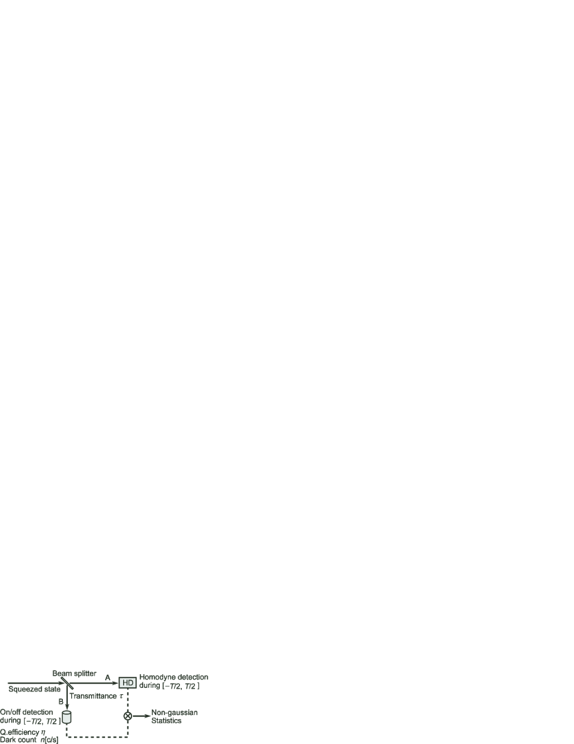
Figure 1: Scheme of the non-Gaussian operation induced by the measurement by the on/off detector.

In order to analyze this scheme we should find an appropriate orthonormal basis set for describing simultaneously the squeezing, the homodyne detection process, and the on/off detection process. The squeezing and homodyne detection of it are described most easily in the frequency domain, whereas the on/off detection is based on the photon counting events appearing in the time domain. The continuum set of the frequency modes $\{\hat{A}(\Omega)\}$ satisfying the commutation relation Eq. (2) is not an appropriate set.

Band-limited signals to $[-B/2,B/2]$ in Hz can be uniquely represented by

$$\hat{A}_{B}(t) = \frac{1}{2\pi}\int_{-\pi B}^{\pi B}d\Omega\hat{A}(\Omega)\mathrm{e}^{-i\Omega t},$$ (8)

$$= \frac{1}{\sqrt{B}}\sum_{k=-\infty}^{\infty}\hat{A}(\frac{k}{B})\theta_{k}(t),$$

where $\theta_{k}(t)$ is the sinc function

$$\theta_{k}(t)=\sqrt{B}\frac{\sin\pi B(t-\frac{k}{B})}{\pi B(t-\frac{k}{B})},$$ (9)

satisfying the orthonormal relation

$$\int_{-\infty}^{\infty}dt\theta_{k}(t)\theta_{l}(t)=\delta_{kl}.$$ (10)

This set, however, is not orthogonal on a finite time duration. So the use of this set is not convenient for describing the events defined on a finite time duration.

Time-limited signals to $[-T/2,T/2]$, on the other hand, can be uniquely represented by

$$\hat{A}_{T}(t)=\sum_{k=-\infty}^{\infty}\hat{A}_{T,k}\phi_{k}(t),$$ (11)

where

$$\phi_{k}(t)=\left\{\begin{array}[]{ll}\displaystyle\frac{1}{\sqrt{T}}\mathrm{exp}(-i\displaystyle\frac{2\pi kt}{T})&\quad-\displaystyle\frac{T}{2}\leq t\leq\displaystyle\frac{T}{2},\\ 0&\quad\mathrm{otherwise},\end{array}\right.$$ (12)

satisfying the orthonormal relation

$$\int_{-T/2}^{T/2}dt\phi_{k}^{\ast}(t)\phi_{l}(t)=\delta_{kl}.$$ (13)

The Fourier coefficient $\hat{A}_{T,k}$ is defined by

$$\hat{A}_{T,k}=\frac{1}{\sqrt{T}}\int_{-T/2}^{T/2}dt\hat{A}(t)\phi_{k}^{\ast}(t),$$ (14)

using the operator in Eq. (6). Although this set is useful to describe the events in the time domain, it makes the analysis complicated when the signal is band-limited. Such a band-limited analysis becomes essential in describing the homodyne current from detector electronics with a finite bandwidth.

The appropriate set to expand the time- and band-limited signals is known as prolate spheroidal wave functions Prolate spheroidal wave functions . These functions frequently apprear in diverse problems in physics and mathematics, and were first introduced to quantum optics by Zhu and Caves Zhu_Caves90 . These functions are defined by the solutions of the integral equation in the time domain

$$\chi_{k}(c)\Psi_{k}(c,t)=\int_{-T/2}^{T/2}dt^{\prime}\frac{\sin\pi B(t-t^{\prime})}{\pi(t-t^{\prime})}\Psi_{k}(c,t^{\prime}),$$ (15)

or equivalently in the frequency domain

$$\chi_{k}(c)\Phi_{k}(c,\Omega)=\int_{-\pi B}^{\pi B}d\Omega^{\prime}\frac{\sin\frac{(\Omega-\Omega^{\prime})T}{2}}{\pi(\Omega-\Omega^{\prime})}\Phi_{k}(c,\Omega^{\prime}).$$ (16)

Actually, given any $T>0$ and any $B>0$, one can find a countably infinite set of real functions for the integral equation

$$\chi_{k}(c)S_{0k}(c,x)=\int_{-1}^{1}dy\frac{\sin c(x-y)}{\pi(x-y)}S_{0k}(c,y),\quad|x|\leq 1,$$ (17)

and a set of real positive numbers satisfying

$$1\geq\chi_{0}(c)>\chi_{1}(c)>\chi_{2}(c)>\cdots,$$ (18)

where $c=\pi BT/2$. The solution $S_{0k}(c,x)$ is called the angular prolate spheroidal wave functions whose properties are summarized in Appendix A. The eigenvalues $\chi_{k}(c)$ are expressed by using a second set of solution $R_{0k}^{(1)}(c,x)$, called the radial prolate spheroidal wave functions, as

$$\chi_{k}(c)=\frac{2c}{\pi}\left[R_{0k}^{(1)}(c,1)\right]^{2}.$$ (19)

$R_{0k}^{(1)}(c,x)$ differ from $S_{0k}(c,x)$ only by a real scale factor.

Using the above functions, the complete and orthonormal set on the finite bandwidth $|\Omega|\leq\pi B$ can be given by

$$\Phi_{k}(c,\Omega)=\sqrt{\frac{2k+1}{B}}S_{0k}(c,\frac{\Omega}{\pi B}),\quad k=0,1,\cdots.$$ (20)

These functions satisfy

$$\Phi_{k}(c,\Omega)=(-1)^{k}\Phi_{k}(c,-\Omega),$$ (21)

$$\frac{1}{2\pi}\int_{-\pi B}^{\pi B}d\Omega\Phi_{k}(c,\Omega)\Phi_{l}(c,\Omega)=\delta_{kl}.$$ (22)

The Fourier transforms of the functions $\Phi_{k}(c,\Omega)$ give mode functions in the time domain. They are explicitly

$$\Psi_{k}(c,t) = \frac{1}{2\pi}\int_{-\pi B}^{\pi B}d\Omega\Phi_{k}(c,\Omega)e^{-i\Omega t}$$ (23)

$$= \sqrt{(2k+1)B}(-i)^{k}R_{0k}^{(1)}(c,1)S_{0k}(c,\frac{2t}{T}).$$

The functions $\Psi_{k}(c,t)$ are defined in the interval $(-\infty,\infty)$ and are orthonormal,

$$\int_{-\infty}^{\infty}dt\Psi_{k}(c,t)\Psi_{l}(c,t)^{\ast}=\delta_{kl}.$$ (24)

They also keep the orthogonality relation over the interval $[-T/2,T/2]$,

$$\int_{-T/2}^{T/2}dt\Psi_{k}(c,t)\Psi_{l}(c,t)^{\ast}=\chi_{k}(c)\delta_{kl}.$$ (25)

For a fixed value of $c$ the $\chi_{k}(c)$ fall off to zero rapidly with increasing $k$ once $k$ has exceeded $2c/\pi$ $(=BT)$. A small value of $\chi_{k}(c)$ implies that $\Psi_{k}(c,t)$ will have most of its weight outside the interval $[-T/2,T/2]$ whereas a value of $\chi_{k}(c)$ near 1 implies that $\Psi_{k}(c,t)$ will be concentrated largely in $[-T/2,T/2]$. The inverse Fourier transformation is

$$\chi_{k}(c)\Phi_{k}(c,\Omega)=\int_{-T/2}^{T/2}dt\Psi_{k}(c,t)e^{i\Omega t}.$$ (26)

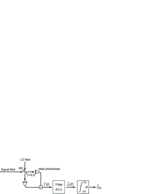
Figure 2: Scheme of balanced homodyne detection.

The time- and band-limited fields are now quantized in terms of these mode $k$. We thus introduce the discrete set of the operators

$$\hat{A}_{k} = \frac{1}{2\pi}\int_{-\pi B}^{\pi B}d\Omega\hat{A}(\Omega)\Phi_{k}(c,\Omega),$$ (27)

$$= \int_{-\infty}^{\infty}dt\hat{A}(t)\Psi_{k}^{\ast}(c,t),$$

which obeys the commutation relation

$$[\hat{A}_{k},\hat{A}_{l}^{\dagger}]=\delta_{kl}.$$ (28)

The operators $\hat{A}(\Omega)$ confined in the finite bandwidth $B$, such as the ones appearing in the squeezing operator Eq. (II), can be expanded as

$$\hat{A}(\Omega)=\sum_{k=0}^{\infty}\hat{A}_{k}\Phi_{k}(c,\Omega).$$ (29)

Let us assume a rectangular squeezing spectrum $\gamma(\Omega)=\gamma$ in Eq.(II). The squeezing operator then factors into a product of single mode squeezing operators

$$\hat{S}=\bigotimes_{k=0}^{\infty}\hat{S}_{k},\quad\hat{S}_{k}=\mathrm{exp}\left[\frac{r_{k}}{2}\left(\hat{A}_{k}^{2}-\hat{A}_{k}^{\dagger 2}\right)\right],$$ (30)

with the squeezing parameter for mode $k$

$$r_{k}=(-1)^{k}\gamma.$$ (31)

The multimode squeezed vacuum state Eq. (4) is now represented by

$$\left|\mathbf{r}\right\rangle=\bigotimes_{k=0}^{\infty}\left|r_{k}\right\rangle,\quad\left|r_{k}\right\rangle=\hat{S}_{k}\left|0\right\rangle.$$ (32)

III Homodyne detection

In order to analyze the mode matching issue in the non-Gaussian operation depicted in Fig. 1, it is essential to know what kind of modes are actually measured in the detectors. In this section we study the homodyne detection from this point of view. The most commonly used homodyne detection scheme is the so-called balanced homodyne detector. Its typical scheme is shown in Fig. 2. In this scheme the signal field $\hat{A}(t)$ is first combined with the LO field $\hat{A}^{\mathrm{L}}(t)$, via a 50:50 beam splitter and the two output beams are converted into photocurrents at each photodetector. The photocurrents from the two detectors are balanced to produce the difference current.

If the photodetector has a $\delta$-function response in time so that it covers the infinite bandwidth, the photocurrents are produced intantaneously. The difference current can then be given by

$$\hat{I}(t)=\hat{A}^{\mathrm{L}\dagger}(t)\hat{A}(t)+\hat{A}^{\dagger}(t)\hat{A}^{\mathrm{L}}(t).$$ (33)

In practical case, however, photodetectors themselves have a non-$\delta$-function response and have a finite bandwidth. Furthermore the difference current is often electrically amplified, and is finally analyzed. The bandwidth of homodyne detector electronics is also limited, usually to a few hundred MHz at most. These effects can be modeled by the response function $h(t)$ such that the instantaneous difference current is filtered through this function Yurke85 ; Ou_Kimble95 . The operator for the filtered current is given by

$$\hat{I}_{h}(t)=\int_{-\infty}^{\infty}d\tau h(t-\tau)\hat{I}(\tau).$$ (34)

This current is integrated over the time duration $[-T/2,T/2]$

$$\hat{I}_{Th}=\int_{-T/2}^{T/2}dt\hat{I}_{h}(t).$$ (35)

This operator directly corresponds to the final observable in the homodyne detection in the present context. Explicit calculation of this current $\hat{I}_{Th}$ will be made for each specific physical model in later sections.

In this section we first assume an ideal homodyne detector with the infinite bandwidth, i.e. $h(t-\tau)=\delta(t-\tau)$, and derive an explicit expression for the final observable. Since the LO field is usually a strong classical field so that its quantum fluctuations can be neglected. We further assume that the LO field has the same or narrower bandwidth than that of the squeezing so that the LO field can be band-limited at least to $|\Omega|\leq\pi B$. One may then expand it as

$$\hat{A}^{\mathrm{L}}(t)=\sum_{k=0}^{\infty}\hat{A}_{k}^{\mathrm{L}}\Psi_{k}(c,t)=\sum_{k=0}^{\infty}\alpha_{k}^{\mathrm{L}}e^{i\phi}\Psi_{k}(c,t).$$ (36)

One should, on the other hand, note that the field operator at the signal port $\hat{A}(t)$ in Eq. (33) can NOT be band-limited because the ideal homodyne detector can be sensitive to the modes even outside the bandwidth of the input squeezed beam, and these modes add the vacuum fluctuations to the homodyne current. So we decompose the field $\hat{A}(t)$ into a sum of the following two components

$$\hat{A}(t)=\hat{A}_{B}(t)+\hat{A}_{V}(t).$$ (37)

Here the first component $\hat{A}_{B}(t)$ is band-limited to the squeezing bandwidth, and hence can be expanded as

$$\hat{A}_{B}(t)=\frac{1}{2\pi}\int_{-\pi B}^{\pi B}d\Omega\hat{A}(\Omega)e^{-i\Omega t}=\sum_{k=0}^{\infty}\hat{A}_{k}\Psi_{k}(c,t).$$ (38)

The second component $\hat{A}_{V}(t)$ consists of the remaining frequency modes

$$\hat{A}_{V}(t)=\frac{1}{2\pi}\left[\int_{-\infty}^{-\pi B}d\Omega+\int_{\pi B}^{\infty}d\Omega\right]\hat{A}(\Omega)e^{-i\Omega t}.$$ (39)

Accordingly the whole Hibert space is divided into two subspaces: one is $\cal H^{\mathrm{S}}$ for the field modes inside the squeezing bandwidth $|\Omega|\leq\pi B$, and the other $\cal H^{\mathrm{V}}$ for the field modes outside the squeezing bandwidth $|\Omega|>\pi B$. The operators $\hat{A}_{B}(t)$ and $\{\hat{A}_{k}\}$ act on $\cal H^{\mathrm{S}}$, while the operator $\hat{A}_{V}(t)$ acts on $\cal H^{\mathrm{V}}$.

The ideal homodyne current is then written as

$$\hat{I}(t) = \sum_{k=0}^{\infty}\sum_{l=0}^{\infty}\alpha_{k}^{\mathrm{L}}e^{-i\phi}\Psi_{k}^{\ast}(c,t)\hat{A}_{l}\Psi_{l}(c,t)$$ (40)

$$+ \sum_{k=0}^{\infty}\alpha_{k}^{\mathrm{L}}e^{-i\phi}\Psi_{k}^{\ast}(c,t)\hat{A}_{V}(t)+\mathrm{h.\,c.},$$

which is defined on the whole Hilbert space $\cal H^{\mathrm{S}}\otimes\cal H^{\mathrm{V}}$. This current is integrated over the time duration $T$ to define the event signals in the time domain

$$\hat{I}_{T} = \int_{-T/2}^{T/2}dt\hat{I}(t)$$ (41)

$$= \sqrt{2}\sum_{k=0}^{\infty}\alpha_{k}^{\mathrm{L}}\chi_{k}(c)\hat{A}_{k}e^{-i\phi}$$

$$+ \sqrt{2}\sum_{k=0}^{\infty}\alpha_{k}^{\mathrm{L}}\sqrt{\chi_{k}(c)[1-\chi_{k}(c)]}\hat{V}_{k}e^{-i\phi}$$

$$+ \mathrm{h.\,c.},$$

where we have used the orthogonality relation Eq. (25), and have introduced the quadrature operators on $\cal H^{\mathrm{V}}$

$$\hat{V}_{k}=\frac{1}{\sqrt{\chi_{k}(c)[1-\chi_{k}(c)]}}\int_{-T/2}^{T/2}dt\hat{A}_{V}(t)\Psi_{k}^{\ast}(c,t),$$ (42)

which satisfies the commutation relation

$$[\hat{V}_{k},\hat{V}_{l}^{\dagger}]=\delta_{kl}.$$ (43)

Define the quadrature operators on $\cal H^{\mathrm{S}}$ for the modes inside the squeezing bandwidth $|\Omega|\leq\pi B$

$$\hat{X}_{k}^{\mathrm{S}}(\phi)=\frac{1}{\sqrt{2}}(\hat{A}_{k}e^{-i\phi}+\hat{A}_{k}^{\dagger}e^{i\phi}),$$ (44)

and the ones on $\cal H^{\mathrm{V}}$ for the modes outside the squeezing bandwidth $|\Omega|>\pi B$

$$\hat{X}_{k}^{\mathrm{V}}(\phi)=\frac{1}{\sqrt{2}}(\hat{V}_{k}e^{-i\phi}+\hat{V}_{k}^{\dagger}e^{i\phi}),$$ (45)

and rewrite Eq. (41) as

$$\hat{I}_{T} = \int_{-T/2}^{T/2}dt\hat{I}(t)$$ (46)

$$= \sqrt{2}\sum_{k=0}^{\infty}\alpha_{k}^{\mathrm{L}}\chi_{k}(c)\hat{X}_{k}^{\mathrm{S}}(\phi)$$

$$+ \sqrt{2}\sum_{k=0}^{\infty}\alpha_{k}^{\mathrm{L}}\sqrt{\chi_{k}(c)[1-\chi_{k}(c)]}\hat{X}_{k}^{\mathrm{V}}(\phi).$$

This integrated homodyne current operator defines the mode which is actually observed in the time domain analysis, the so called LO matched mode Smithey93_PRL_DC_Homodyne ; Raymer95_JOSAB_HomodyneModeMatch .

We define the quadrature operator for the LO matched mode in the following way. Define the weight factors

$$w_{k}^{\mathrm{S}}=\frac{\alpha_{k}^{\mathrm{L}}\chi_{k}(c)}{\sqrt{\displaystyle\sum_{k=0}^{\infty}(\alpha_{k}^{\mathrm{L}})^{2}\chi_{k}(c)}},$$ (47)

and

$$w_{k}^{\mathrm{V}}=\frac{\alpha_{k}^{\mathrm{L}}{\sqrt{\chi_{k}(c)[1-\chi_{k}(c)]}}}{\sqrt{\displaystyle\sum_{k=0}^{\infty}\left(\alpha_{k}^{\mathrm{L}}\right)^{2}\chi_{k}(c)}},$$ (48)

such that

$$\sum_{k=0}^{\infty}\left[\left(w_{k}^{\mathrm{S}}\right)^{2}+\left(w_{k}^{\mathrm{V}}\right)^{2}\right]=1.$$ (49)

In order to simplify the notation on the Hilbert space $\cal H^{\mathrm{S}}\otimes\cal H^{\mathrm{V}}$, let us further introduce vector notations

$$\hat{\mathbf{X}}(\phi)\equiv\left[\begin{array}[]{c}\hat{X}_{0}(\phi)\\ \hat{X}_{1}(\phi)\\ \hat{X}_{2}(\phi)\\ \vdots\\ \end{array}\right]\equiv\left[\begin{array}[]{c}\hat{X}_{0}^{\mathrm{S}}(\phi)\\ \hat{X}_{1}^{\mathrm{S}}(\phi)\\ \vdots\\ \hat{X}_{0}^{\mathrm{V}}(\phi)\\ \hat{X}_{1}^{\mathrm{V}}(\phi)\\ \vdots\\ \end{array}\right],$$ (50)

$$\bm{\epsilon}\equiv\left[\begin{array}[]{c}\epsilon_{0}\\ \epsilon_{1}\\ \epsilon_{2}\\ \vdots\\ \end{array}\right]\equiv\left[\begin{array}[]{c}w_{0}^{\mathrm{S}}\\ w_{1}^{\mathrm{S}}\\ \vdots\\ w_{0}^{\mathrm{V}}\\ w_{1}^{\mathrm{V}}\\ \vdots\\ \end{array}\right],$$ (51)

and

$${\mathbf{x}}(\phi)\equiv\left[\begin{array}[]{c}x_{0}(\phi)\\ x_{1}(\phi)\\ x_{2}(\phi)\\ \vdots\\ \end{array}\right]\equiv\left[\begin{array}[]{c}x_{0}^{\mathrm{S}}(\phi)\\ x_{1}^{\mathrm{S}}(\phi)\\ \vdots\\ x_{0}^{\mathrm{V}}(\phi)\\ x_{1}^{\mathrm{V}}(\phi)\\ \vdots\\ \end{array}\right],$$ (52)

where

$$\hat{X}_{k}^{\mathrm{S}}(\phi)\left|x_{k}^{\mathrm{S}}(\phi)\right\rangle=x_{k}^{\mathrm{S}}(\phi)\left|x_{k}^{\mathrm{S}}(\phi)\right\rangle,$$ (53)

and

$$\hat{X}_{k}^{\mathrm{V}}(\phi)\left|x_{k}^{\mathrm{V}}(\phi)\right\rangle=x_{k}^{\mathrm{V}}(\phi)\left|x_{k}^{\mathrm{V}}(\phi)\right\rangle.$$ (54)

Here we have

$$[\hat{X}_{k}(\phi),\hat{X}_{l}(\phi+{\pi\over 2})]=i\delta_{kl}.$$ (55)

The integrated homodyne current Eq. (46) is then written as

$$\hat{I}_{T}={\sqrt{2\displaystyle\sum_{k=0}^{\infty}\left(\alpha_{k}^{\mathrm{L}}\right)^{2}\chi_{k}(c)}}\tilde{X}_{0}(\phi)$$ (56)

where

$$\tilde{X}_{0}(\phi)={}^{t}\bm{\epsilon}\cdot\hat{\mathbf{X}}(\phi)$$ (57)

is the quadrature operator for the LO matched mode, which is defined on the entire Hilbert space $\cal H^{\mathrm{S}}\otimes\cal H^{\mathrm{V}}$. It is this operator that corresponds to the final observable in the homodyme detector for the time domain non-Gaussian operation. In the following calculation we only need quadrature operators at $\phi=0$, those are simply represented by

$$\hat{X}_{k} = \hat{X}_{k}(0),$$

$$\hat{P}_{k} = \hat{X}_{k}({\pi\over 2}),$$

$$\tilde{X}_{0} = \tilde{X}_{0}(0),$$

$$\tilde{P}_{0} = \tilde{X}_{0}({\pi\over 2}).$$

The POVM and the resulting measurement statistics for the integrated homodyne current is described by using the eigenstates of $\tilde{X}_{0}$

$$\tilde{X}_{0}\left|x_{0}^{\prime}\right)=x_{0}^{\prime}\left|x_{0}^{\prime}\right).$$ (59)

The round ket notation $\left|\,\,\,\right)$ is used to discriminate these eigenstates from the ones for the quadrature operators which describe the input squeezed $\{\hat{X}_{0}^{\mathrm{S}},\hat{X}_{1}^{\mathrm{S}},\cdots\}$ and the vacuum $\{\hat{X}_{0}^{\mathrm{V}},\hat{X}_{1}^{\mathrm{V}},\cdots\}$ fields

$$\hat{X}_{k}\left|x_{k}\right\rangle=x_{k}\left|x_{k}\right\rangle,\quad(k=0,1,\cdots).$$ (60)

In order to represent the quantum state of measured mode, and to calculate the corresponding Wigner function, we have to derive the formula to connect $\{\left|x_{0}^{\prime}\right)\}$ with $\{\left|x_{0}\right\rangle,\left|x_{1}\right\rangle,\cdots\}$. For this purpose we consider a real unitary transformation

$$\left[\begin{array}[]{c}\tilde{X}_{0}\\ \tilde{X}_{1}\\ \tilde{X}_{2}\\ \vdots\end{array}\right]=\left[\begin{array}[]{cccc}\epsilon_{0}&\epsilon_{1}&\epsilon_{2}&\cdots\\ u_{10}&u_{11}&u_{12}&\cdots\\ u_{20}&u_{21}&u_{22}&\cdots\\ \vdots&\vdots&\vdots&\ddots\\ \end{array}\right]\left[\begin{array}[]{c}\hat{X}_{0}\\ \hat{X}_{1}\\ \hat{X}_{2}\\ \vdots\end{array}\right],$$ (61)

which includes the linear relation of Eq. (57) in the 0th component. We denote this equation as

$$\tilde{\mathbf{X}}={\mathbf{U}}\hat{\mathbf{X}}.$$ (62)

Such a unitary transformation is not unique, but here we need not to know its explicit components. As in Eq. (59), the eigenstates of $\tilde{X}_{k}$ are denoted by

$$\tilde{X}_{k}\left|x_{k}^{\prime}\right)=x_{k}^{\prime}\left|x_{k}^{\prime}\right),\quad(k=0,1,\cdots).$$ (63)

The two sets of operators $\{\hat{X}_{k}\}$ and $\{\tilde{X}_{k}\}$ can be considered to act on the same Hilbert space $\cal H^{\mathrm{S}}\otimes\cal H^{\mathrm{V}}$. In fact, the tensor product states of all the modes for the two sets of eigenstates are related with each other by

$$\left|\mathbf{x}\right\rangle \equiv \bigotimes_{k=0}^{\infty}\left|x_{k}\right\rangle$$ (64)

$$= \exp(-i{}^{t}\mathbf{x}\cdot\hat{\mathbf{P}})\left|\mathbf{0}\right\rangle$$

$$= \exp(-i{}^{t}\mathbf{x}\mathbf{U}^{\dagger}\cdot\mathbf{U}\hat{\mathbf{P}})\left|\mathbf{0}\right\rangle$$

$$= \exp(-i{}^{t}\mathbf{x^{\prime}}\cdot\tilde{\mathbf{P}})\left|\mathbf{0}\right\rangle$$

$$= \bigotimes_{k=0}^{\infty}\left|x^{\prime}_{k}\right)$$

$$= \left|\mathbf{x^{\prime}}\right),$$

where

$$\mathbf{x^{\prime}}=\mathbf{U}\mathbf{x}.$$ (65)

Given an input multimode field in a quantum state $\hat{\rho}$ on $\cal H^{\mathrm{S}}\otimes\cal H^{\mathrm{V}}$, the integrated homodyne current delivers information only on the LO matched mode in $\hat{\rho}$. Therefore what we actually observe is a reduced density operator on the subspace $\cal H^{\mathrm{L}}$ spanned by $\left|x_{0}^{\prime}\right)$

$$\tilde{\rho}\equiv\int dx^{\prime}_{1}\int dx^{\prime}_{2}\cdots\left(x^{\prime}_{1},x^{\prime}_{2},\cdots\right|\hat{\rho}\left|x^{\prime}_{1},x^{\prime}_{2},\cdots\right).$$ (66)

The matrix element in terms of the quadrature eigenstates for the LO matched mode on the subspace $\cal H^{\mathrm{L}}$ is given by

$$\left(x\right|\tilde{\rho}\left|y\right) = \int dx^{\prime}_{0}\int dx^{\prime}_{1}\int dx^{\prime}_{2}\cdots\delta(x-x^{\prime}_{0})$$ (67)

$$\times\left(x^{\prime}_{0},x^{\prime}_{1},x^{\prime}_{2},\cdots\right|\hat{\rho}\left|y,x^{\prime}_{1},x^{\prime}_{2},\cdots\right)$$

$$= \int d\mathbf{x^{\prime}}\delta(x-{}^{t}\bm{\epsilon}\cdot\mathbf{x})$$

$$\times\left(\mathbf{x}^{\prime}\right|\hat{\rho}\left|y,x^{\prime}_{1},x^{\prime}_{2},\cdots\right),$$

where we have used the relation of the eigenvalues for the LO matched mode

$$x^{\prime}_{0}=\sum_{l=0}^{\infty}\epsilon_{l}x_{l}={}^{t}\bm{\epsilon}\cdot\mathbf{x}.$$ (68)

We then transform the variables $\mathbf{x^{\prime}}={}^{t}(x^{\prime}_{0},x^{\prime}_{1},x^{\prime}_{2},\cdots)$ into $\mathbf{x}={}^{t}(x_{0},x_{1},x_{2},\cdots)$ by Eq. (65). Firstly we have

$$\int d\mathbf{x^{\prime}}=\int d\mathbf{x},$$ (69)

because the Jacobian of this variable transformation is $|\mathrm{det}\mathbf{U}|=1$. Secondly

$$\left(\mathbf{x}^{\prime}\right|=\left\langle\mathbf{x}\right|$$ (70)

according to Eq. (64). Thirdly the quadrature eigenstates $\left|y,x^{\prime}_{1},x^{\prime}_{2},\cdots\right)$ is converted as

$$\left|y,x^{\prime}_{1},x^{\prime}_{2},\cdots\right) = \bigotimes_{k=0}^{\infty}\left|x_{k}+\bigl{(}y-{}^{t}\bm{\epsilon}\cdot\mathbf{x}\bigr{)}\epsilon_{k}\right\rangle$$ (71)

$$= \left|\mathbf{x}+(y-{}^{t}\bm{\epsilon}\cdot\mathbf{x})\bm{\epsilon}\right\rangle,$$

because

$$\left[\begin{array}[]{c}y\\ x_{1}^{\prime}\\ x_{2}^{\prime}\\ \vdots\end{array}\right]=\mathbf{U}\left[\begin{array}[]{c}x_{0}+(y-x_{0}^{\prime})\epsilon_{0}\\ x_{1}+(y-x_{0}^{\prime})\epsilon_{1}\\ x_{2}+(y-x_{0}^{\prime})\epsilon_{2}\\ \vdots\end{array}\right],$$ (72)

which can be obtained by eliminating the terms $\sum_{k=1}^{\infty}u_{kj}x_{k}^{\prime}$ in the following two equations

$$\mathbf{U}^{\dagger}\left[\begin{array}[]{c}y\\ x_{1}^{\prime}\\ x_{2}^{\prime}\\ \vdots\end{array}\right]=\left[\begin{array}[]{c}\epsilon_{0}y+\sum_{k=1}^{\infty}u_{k0}x_{k}^{\prime}\\ \epsilon_{1}y+\sum_{k=1}^{\infty}u_{k1}x_{k}^{\prime}\\ \epsilon_{2}y+\sum_{k=1}^{\infty}u_{k2}x_{k}^{\prime}\\ \vdots\end{array}\right],$$ (73)

and

$$\left[\begin{array}[]{c}x_{0}\\ x_{1}\\ x_{2}\\ \vdots\end{array}\right]=\mathbf{U}^{\dagger}\left[\begin{array}[]{c}x_{0}^{\prime}\\ x_{1}^{\prime}\\ x_{2}^{\prime}\\ \vdots\end{array}\right]=\left[\begin{array}[]{c}\epsilon_{0}x_{0}^{\prime}+\sum_{k=1}^{\infty}u_{k0}x_{k}^{\prime}\\ \epsilon_{1}x_{0}^{\prime}+\sum_{k=1}^{\infty}u_{k1}x_{k}^{\prime}\\ \epsilon_{2}x_{0}^{\prime}+\sum_{k=1}^{\infty}u_{k2}x_{k}^{\prime}\\ \vdots\end{array}\right],$$ (74)

The matrix element Eq. (67) is finally given by

$$\left(x\right|\tilde{\rho}\left|y\right)=\int d\mathbf{x}\delta(x-{}^{t}\bm{\epsilon}\cdot\mathbf{x})\left\langle\mathbf{x}\right|\hat{\rho}\left|\mathbf{x}+(y-x)\bm{\epsilon}\right\rangle.$$ (75)

This formulus allows one to calculate the statistics of the LO matched mode in the time-integrated homodyne detection (the left-hand side), using the quantum state originally represented in terms of the plorate spheroidal wave function modes (the right-hand side).

IV On/off detector

In contrast to that homodyne detectors can be implemented in the near ideal condition at least for the near infrared wavelengths at present using Si p-i-n photodiodes, on/off detectors usually suffer from imperfect efficiency and dark counts. In the present context where an on/off detector is used to select events, dark counts essentially influence the quality of the non-Gaussian operation.

The number operator for photons arriving at the detector during the interval $T$ is

$$\hat{n}_{T} = \int_{-T/2}^{T/2}dt\hat{a}^{\dagger}(t)\hat{a}(t)$$ (76)

$$= \int_{-T/2}^{T/2}dt\hat{A}^{\dagger}(t)\hat{A}(t).$$

Although the signal field $\hat{A}(t)$ appearing in the homodyne current cannot be band-limited to the squeezing bandwidth, it CAN be here, because the vacuum field components outside the squeezing bandwidth does not induce photon counts. So $\hat{A}(t)$ can be replaced by $\hat{A}_{B}(t)$, and can be expanded as in Eq. (38). We then obtain

$$\hat{n}_{T}=\sum_{k=0}^{\infty}\chi_{k}(c)\hat{A}_{k}^{\dagger}\hat{A}_{k}.$$ (77)

For mode $k$ we define

$$\hat{n}_{k}=\hat{A}_{k}^{\dagger}\hat{A}_{k},\quad\hat{n}_{k}\left|n_{k}\right\rangle=n_{k}\left|n_{k}\right\rangle.$$ (78)

For a photon counter with a finite quantum efficiency $\eta_{k}$ for mode $k$, the POVM element registering $n$ photocarriers due to photons in mode $k$ is given by Barnett98_PhptonCounter ,

$$\hat{\Pi}_{k}(n;\eta_{k})=\sum_{m=n}^{\infty}\left(\begin{array}[]{c}m\cr n\end{array}\right)\eta_{k}^{n}(1-\eta_{k})^{m-n}|m\rangle\langle m|.$$ (79)

The effective quantum efficiency $\eta_{k}$ for mode $k$ here is of the form $\eta_{k}=\eta\chi_{k}(c)$, where $\eta$ is the net detection efficiency determined by the total coupling efficiency of photons through optical components to the photondetector and the intrinsic quantum efficiency of the photondetector. This is assumed to be constant over the squeezing bandwidth. The factor $\chi_{k}(c)$ represents the weight of mode $k$ on the counting interval $[-T/2,T/2]$. Taking the effect of the dark counts into account, the POVM registering $n$ counts is then given by

$$\hat{\Pi}_{k}(n;\eta_{k},\nu_{k})=\sum_{n^{\prime}=0}^{n}e^{-\nu_{k}}\frac{\nu_{k}^{n-n^{\prime}}}{(n-n^{\prime})!}\hat{\Pi}_{k}(n^{\prime};\eta_{k}),$$ (80)

where $\nu_{k}$ is the mean number of the dark counts for photons in mode $k$. (The dark counts may occur regardless of the bandwidth of the input signal field, however, they can be taken into account by adjusting the values $\nu_{k}$ for the band-limited modes such that the total dark count rate in practical detecotrs is properly modeled.) These elements satisfy the completeness relation for each mode $k$,

$$\sum_{n=0}^{\infty}\hat{\Pi}_{k}(n;\eta_{k},\nu_{k})=\hat{I}_{k}.$$ (81)

The multimode on/off detector placed at path B in Fig. 1 is finally modeled by a binary POVM with parameters $\bm{\eta}=(\eta_{0},\eta_{1},\cdots)$ and $\bm{\nu}=(\nu_{0},\nu_{1},\cdots)$,

$$\hat{\Pi}_{\mathrm{off}}^{\mathrm{B}}(\bm{\eta},\bm{\nu}) = \bigotimes_{k=0}^{\infty}\hat{\Pi}_{k}^{\mathrm{B}}(0;\eta_{k},\nu_{k}),$$

$$\hat{\Pi}_{\mathrm{on}}^{\mathrm{B}}(\bm{\eta},\bm{\nu}) = \hat{I}^{\mathrm{B}}-\hat{\Pi}_{\mathrm{off}}^{\mathrm{B}}(\bm{\eta},\bm{\nu}).$$ (82)

V Wigner function of the non-Gaussian state

We now explicitly calculate the non-Gaussian output state conditionally obtained by the on/off detector specified in the previous section, and derive an expression of the Wigner function measured by the ideal homodyne detector described in Section III. For convenience of mathematical handling, we express the squeezed vacuum state

$$\left|\mathbf{r}^{\mathrm{S}}\right\rangle=\bigotimes_{k=0}^{\infty}\left|r_{k}\right\rangle,\quad\left|r_{k}\right\rangle=\hat{S}_{k}\left|0\right\rangle,$$ (83)

in terms of the coherent state basis $\left|\alpha_{k}\right\rangle$ on the Hibert space $\cal H^{\mathrm{S}}$. The component of mode $k$ can be expanded as

$$\left|r_{k}\right\rangle = \frac{(1-{\lambda_{k}}^{2})^{1\over 4}}{\pi}$$ (84)

$$\times \int_{-\infty}^{\infty}d^{2}\alpha_{k}\exp\left[-\frac{|\alpha_{k}|^{2}}{2}-\frac{\lambda_{k}}{2}\alpha_{k}^{\ast 2}\right]\left|\alpha_{k}\right\rangle,$$

with $\lambda_{k}=\tanh r_{k}$. As in Fig. 1, the squeezed vacuum state is beamsplitted into path A and B, resulting in a state

$$\left|\rho^{\mathrm{S}}\right\rangle_{\mathrm{AB}}=\bigotimes_{k=0}^{\infty}\frac{(1-{\lambda_{k}}^{2})^{1\over 4}}{\pi}\int_{-\infty}^{\infty}d^{2}\alpha_{k}\exp\biggr{[}-\frac{|\alpha_{k}|^{2}}{2}$$

$$-\frac{\lambda_{k}}{2}\alpha_{k}^{\ast 2}\biggr{]}\left|\sqrt{\tau}\alpha_{k}\right\rangle_{\mathrm{A}}\left|-\sqrt{1-\tau}\alpha_{k}\right\rangle_{\mathrm{B}},$$ (85)

where $\tau$ is the transmittance.

The photon subtracted non-Gaussian state at path A is given by

$$\hat{\rho}_{\mathrm{A}}^{\mathrm{S}}=\frac{1}{P_{\mathrm{det}}}{\rm\,Tr}\,_{\mathrm{B}}\left[\left|\rho^{\mathrm{S}}\right\rangle_{\mathrm{(AB)}}\left\langle\rho^{\mathrm{S}}\right|\hat{I}^{\mathrm{A}}\otimes\hat{\Pi}_{\mathrm{on}}^{\mathrm{B}}(\bm{\eta},\bm{\nu})\right],$$ (86)

where

$$P_{\mathrm{det}}={\rm\,Tr}\,_{\mathrm{AB}}\left[\left|\rho^{\mathrm{S}}\right\rangle_{\mathrm{(AB)}}\left\langle\rho^{\mathrm{S}}\right|\hat{I}^{\mathrm{A}}\otimes\hat{\Pi}_{\mathrm{on}}^{\mathrm{B}}(\bm{\eta},\bm{\nu})\right],$$ (87)

is the probability of having the “on” signals. Using Eqs. (V) and (IV), $\hat{\rho}_{\mathrm{A}}^{\mathrm{S}}$ can be represented as

$$\hat{\rho}_{\mathrm{A}}^{\mathrm{S}}=\frac{1}{P_{\mathrm{det}}}\left(\bigotimes_{k=0}^{\infty}\hat{R}_{k}(0,0)-\bigotimes_{k=0}^{\infty}\hat{R}_{k}(\eta_{k},\nu_{k})\right),$$ (88)

with

$$\hat{R}_{k}(\eta_{k},\nu_{k}) = \frac{\sqrt{1-{\lambda_{k}}^{2}}}{\pi^{2}}\int d^{2}\alpha_{k}\int d^{2}\beta_{k}\exp\Biggl{[}-\frac{2-\tau}{2}$$ (89)

$$\times \biggl{(}|\alpha_{k}|^{2}+|\beta_{k}|^{2}\biggr{)}+(1-\tau)(1-\eta_{k})\beta_{k}^{\ast}\alpha_{k}$$

$$- \frac{\lambda_{k}}{2}(\alpha_{k}^{\ast 2}+\beta_{k}^{2})$$

$$- \nu_{k}\Biggr{]}\left|{\sqrt{\tau}}\alpha_{k}\right\rangle_{\mathrm{A}}\left\langle{\sqrt{\tau}}\beta_{k}\right|.$$

The state $\hat{\rho}_{\mathrm{A}}^{\mathrm{S}}$ is finally measured by the time-integrated homodyne detection to construct the Wigner function. As explained in Section III, the ideal homodyne detector is sensitive not only to the state $\hat{\rho}_{\mathrm{A}}^{\mathrm{S}}$ but also to the vacuum states $\left|\mathbf{0}^{\mathrm{V}}\right\rangle$ outside the squeezing bandwidth. So the input state into the ideal homodyne detector must be

$$\hat{\rho}_{\mathrm{A}}=\hat{\rho}_{\mathrm{A}}^{\mathrm{S}}\otimes\left|\mathbf{0}^{\mathrm{V}}\right\rangle\left\langle\mathbf{0}^{\mathrm{V}}\right|$$ (90)

The time-integrated homodyne current delivers information only on the LO matched mode, whose state is represented by the reduced density operator $\tilde{\rho}_{\mathrm{A}}$ defined by Eq. (66). Its matrix element in terms of the quadrature eigenstates is given by Eq. (75). The Wigner function of the reduced density operator for the LO matched mode is then given by

$$W(x,p)=\frac{1}{2\pi}\int_{-\infty}^{\infty}d\xi e^{-ip\xi}\left(x+{\xi\over 2}\right|\tilde{\rho}_{\mathrm{A}}\left|x-{\xi\over 2}\right),$$ (91)

where the matrix element is given by

$$\left(x+{\xi\over 2}\right|\tilde{\rho}_{\mathrm{A}}\left|x-{\xi\over 2}\right)$$ (92)

$$=\int d\mathbf{x}\delta(x+{\xi\over 2}-{}^{t}\bm{\epsilon}\cdot\mathbf{x})\left\langle\mathbf{x}\right|\hat{\rho}_{\mathrm{A}}\left|\mathbf{x}-\xi\bm{\epsilon}\right\rangle$$

$$=\int d\mathbf{x}^{\mathrm{S}}\int d\mathbf{x}^{\mathrm{V}}\delta(x+{\xi\over 2}-{}^{t}\mathbf{w}^{\mathrm{S}}\cdot\mathbf{x}^{\mathrm{S}}-{}^{t}\mathbf{w}^{\mathrm{V}}\cdot\mathbf{x}^{\mathrm{V}})$$

$$\quad\times\left\langle\mathbf{x}^{\mathrm{S}}\right|\hat{\rho}_{\mathrm{A}}^{\mathrm{S}}\left|\mathbf{x}^{\mathrm{S}}-\xi\mathbf{w}^{\mathrm{S}}\right\rangle$$

$$\quad\times\left\langle\mathbf{x}^{\mathrm{V}}\right|\mathbf{0}^{\mathrm{V}}\rangle\langle\mathbf{0}^{\mathrm{V}}\left|\mathbf{x}^{\mathrm{V}}-\xi\mathbf{w}^{\mathrm{V}}\right\rangle.$$

In the second equality we have replaced the abbreviated notations $\{\epsilon_{k}\}$ and $\{x_{k}\}$ introduced in Eqs. (51) and (52) with the explicit ones $\{w_{k}^{\mathrm{S}},w_{k}^{\mathrm{V}}\}$ and $\{x_{k}^{\mathrm{S}},x_{k}^{\mathrm{V}}\}$. Substituting the expression of Eq. (88) into the above equation, we have

$$\left(x+{\xi\over 2}\right|\tilde{\rho}_{\mathrm{A}}\left|x-{\xi\over 2}\right)$$

$$=\frac{1}{2\pi}\int_{-\infty}^{\infty}dqe^{i(x+{\xi\over 2})q}\prod_{l=0}^{\infty}\int_{-\infty}^{\infty}dx_{l}^{\mathrm{V}}\mathrm{exp}(-iqw_{l}^{\mathrm{V}}x_{l}^{\mathrm{V}})$$

$$\quad\quad\times\left\langle x_{l}^{\mathrm{V}}\right|0_{l}^{\mathrm{V}}\rangle\langle 0_{l}^{\mathrm{V}}\left|x_{l}^{\mathrm{V}}-\xi w_{l}^{\mathrm{V}}\right\rangle$$

$$\times\Biggl{\{}\prod_{k=0}^{\infty}\int_{-\infty}^{\infty}dx_{k}^{\mathrm{S}}\mathrm{exp}(-iqw_{k}^{\mathrm{S}}x_{k}^{\mathrm{S}})$$

$$\quad\quad\times\left\langle x_{k}^{\mathrm{S}}\right|\hat{R}_{k}(0,0)\left|x_{k}^{\mathrm{S}}-\xi w_{k}^{\mathrm{S}}\right\rangle$$

$$\quad-\prod_{k=0}^{\infty}\int_{-\infty}^{\infty}dx_{k}^{\mathrm{S}}\mathrm{exp}(-iqw_{k}^{\mathrm{S}}x_{k}^{\mathrm{S}})$$

$$\quad\quad\times\left\langle x_{k}^{\mathrm{S}}\right|\hat{R}_{k}(\eta_{k},\nu_{k})\left|x_{k}^{\mathrm{S}}-\xi w_{k}^{\mathrm{S}}\right\rangle\Biggr{\}},$$ (93)

where we have used the Fourier expansion for the delta function in Eq. (92). After straightforward calculations of Gaussian integrations, the Wigner function can be finally represented as

$$W(x,p)=\frac{1}{P_{\mathrm{det}}}\left[R(x,p;\bm{0},\bm{0})-R(x,p;\bm{\eta},\bm{\nu})\right],$$ (94)

where

$$R(x,p;\bm{\eta},\bm{\nu}) = \frac{\cal{N}(\bm{\eta},\bm{\nu})}{\pi\sqrt{\zeta_{+}(\bm{\eta})\zeta_{-}(\bm{\eta})}}$$ (95)

$$\times \exp\Biggl{[}-\frac{x^{2}}{\zeta_{-}(\bm{\eta})}-\frac{p^{2}}{\zeta_{+}(\bm{\eta})}\Biggr{]},$$

with

$$\zeta_{\pm}(\bm{\eta})=1\pm\tau\sum_{k=0}^{\infty}\frac{2\lambda_{k}}{\gamma_{\pm}(\eta_{k})}\left(w_{k}^{\mathrm{S}}\right)^{2},$$ (96)

$$\gamma_{\pm}(\eta_{k})=1\mp\lambda_{k}\pm(1-\tau)\eta_{k}\lambda_{k},$$ (97)

and

$${\cal N}(\bm{\eta},\bm{\nu})=\prod_{k=0}^{\infty}\sqrt{\frac{1-\lambda_{k}^{2}}{\gamma_{+}(\eta_{k})\gamma_{-}(\eta_{k})}}e^{-\nu_{k}},$$ (98)

and

$$R(x,p;\bm{0},\bm{0})$$ (99)

$$= \frac{\displaystyle\frac{1}{\pi}\exp\Biggl{(}-\frac{x^{2}}{1-\tau+\sigma_{-}^{2}\tau}-\frac{p^{2}}{1-\tau+\sigma_{+}^{2}\tau}\Biggr{)}}{\sqrt{(1-\tau+\sigma_{-}^{2}\tau)(1-\tau+\sigma_{+}^{2}\tau)}},$$

with

$$\sigma_{\pm}^{2}\equiv\sum_{k=0}^{\infty}\left[\left(w_{k}^{\mathrm{S}}\right)^{2}e^{\pm 2r_{k}}+\left(w_{k}^{\mathrm{V}}\right)^{2}\right].$$ (100)

The probability of having the “on” signal is given by

$$P_{\mathrm{det}}=1-{\cal N}(\bm{\eta},\bm{\nu}).$$ (101)

Thus the relevant quantum states can be represented in terms of the discrete set of the prolate spheriodal wave function modes. This discretization becomes more prominent as the time- and band-limitation gets more stringent. In fact, for $BT\ll 1$, only the 0th mode becomes dominant as shown later. If one could make the photon-subtracted squeezed state pure in this 0th single mode, and could selectively measure the 0th mode by the homodyne detector, then the ideal mode matching should be realized. But for this, it is not sufficient to simply put $BT\ll 1$. Some additional care must be taken, depending on specific physical models actually used. So in the following two sections, we apply the result in this section to two kinds of models: CW and pulsed schemes.

VI CW scheme

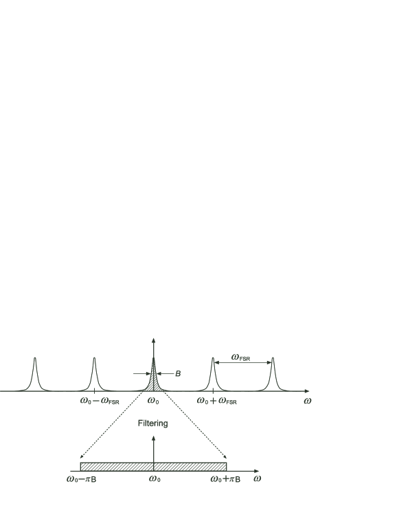
Figure 3: Frequency spectrum of the squeezed state generated by an optical parametric oscillator cavity.

A typical example of CW scheme is an optical parametric oscillator cavity containing a $\chi^{(2)}$ nonlinear medium, continuously pumped by a single mode field at optical frequency $2\omega_{0}$. A pump photon is down-converted into quantum correlated twin photons at optical frequencies $\omega_{0}+\Omega$ and $\omega_{0}-\Omega$, resulting in an frequency entangled state of squeezed vacuum via cavity enhancement. In a commonly used temperature-controlled phase matching scheme, such twin photons are generated over a wide range of frequencies something like a few tens of GHz around the degenerate frequency $\omega_{0}$. A typical frequency spectrum is shown in Fig. 3. It consists of multi resonant peaks separated by the frequency $\omega_{\mathrm{FSR}}$ of a free spectrum range. For a commmon bow-tie configuration with a round-trip length of $\sim$500 mm, $\omega_{\mathrm{FSR}}$ is about 600 MHz, and a width of each resonant peak is $B\sim 10$ MHz. Such a wide band CW squeezed state is a source state for the non-Gaussian operation here. The events in time domain are defined by imposing the finite time duration $T$ on the on/off detector.

Let us first consider time-integrated homodyne detection with the infinite detection bandwidth as shown in Fig. 4. The LO is a CW single mode field at optical frequency $\omega_{0}$. In the rotating frame, it is written as

$$\hat{A}^{\mathrm{L}}(\Omega)=\alpha^{\mathrm{L}}e^{i\phi}\delta(\Omega).$$ (102)

A CW signal beam is combined with the LO field, producing the CW current,

$$\hat{I}(t)=\frac{1}{2\pi}\int_{-\infty}^{\infty}d\Omega\hat{I}(\Omega)e^{-i\Omega t},$$ (103)

with

$$\hat{I}(\Omega)=\frac{\alpha^{\mathrm{L}}}{2\pi}\left[\hat{A}(\Omega)e^{-i\phi}+\hat{A}^{\dagger}(-\Omega)e^{i\phi}\right],$$ (104)

and this current is integrated over $[-T/2,T/2]$

$$\hat{I}_{T}=\frac{\alpha^{\mathrm{L}}}{2\pi}\int_{-\infty}^{\infty}d\Omega\left[\hat{A}(\Omega)e^{-i\phi}+\hat{A}^{\dagger}(\Omega)e^{i\phi}\right]\frac{\sin\frac{\Omega T}{2}}{\pi\Omega}.$$ (105)

As seen from this expression, it depends on the choice of $T$ what frequency modes dominate in $\hat{I}_{T}$. For $T\gg\omega_{\mathrm{FSR}}^{-1}$, contribution from the modes in the resonant peaks at $\omega_{0}\pm n\omega_{\mathrm{FSR}}$ $(n=1,2,...)$ is negligible. For $T>B^{-1}$, the modes inside the resonant peak centered at $\omega_{0}$ dominate. For an intermediate region, $\omega_{\mathrm{FSR}}^{-1}<T<B^{-1}$, the modes in the free spectrum range, which are in vacuum states, also contribute to $\hat{I}_{T}$ in addition to the ones in the center resonant peak. Thus under the assumption $T\gg\omega_{\mathrm{FSR}}^{-1}$, it is enough, concerning the time-integrated homodyne detection, to consider a squeezed state whose spectrum is confined to the center resonant peak shaded in Fig. 3.

Figure 4: Time-integrated homodyne detection in a CW setting. The detection bandwidth is assumed to be infinite.

One should, however, note that this is not true for the on/off detector. The on/off detector is sensitive to all the modes regardless of the measurement duration $T$. Therefore for a good frequency mode matching, the tapped-off beam must be optically filtered in front of the on/off detector such that only the center resonant peak shaded in Fig. 3 is guided into the on/off detector. This can be made by employing an appropriate set of filtering cavities. This is actually the assumption under the model of band-limited squeezing introduced in Eq. (II) or (II). We further simplify the squeezing spectrum so as to be the flat band over $[-\pi B,\pi B]$, as shown in the lower part of Fig. 3, which is actually the model of Eq. (30).

VI.1 LO matched mode measured by homodyne detector with the infinite bandwidth

Before analyzing the non-Gaussian operation, let us consider a simple case where the squeezed vacuum state is directly measured by the homodyne detector without the photon-subtraction by the on/off detector. The Wigner function in this case is given simply by $R(x,p;\bm{0},\bm{0})$ in Eq. (99) and (100) with $\tau=1$. Using Eq. (27), the $k$th coefficient of the CW single mode LO field in Eq. (102) is given by

$$\alpha_{k}^{\mathrm{L}}=\frac{\alpha^{\mathrm{L}}}{2\pi}\Phi_{k}(c,0)=\frac{\alpha^{\mathrm{L}}}{2\pi}\sqrt{\frac{2k+1}{B}}P_{k}(0),$$ (106)

where $P_{k}(x)$ is the $k$th Legendre polynomial and

$$P_{k}(0)=\left\{\begin{array}[]{ll}(-1)^{\frac{k}{2}}\displaystyle\frac{(k-1)!!}{k!!}&\quad(k:\mathrm{even}),\\ 0&\quad(k:\mathrm{odd}).\end{array}\right.$$ (107)

The variance is then expressed as

$$\sigma_{-}^{2}=e^{-2\gamma}\mathrm{w}^{\mathrm{S}}+\mathrm{w}^{\mathrm{V}},$$ (108)

where

$$\mathrm{w}^{\mathrm{S}}\equiv\sum_{k:\mathrm{even}}\left(w_{k}^{\mathrm{S}}\right)^{2}=\frac{\displaystyle\sum_{k:\mathrm{even}}(2k+1)P_{k}(0)^{2}\chi_{k}(c)^{2}}{\displaystyle\sum_{k:\mathrm{even}}(2k+1)P_{k}(0)^{2}\chi_{k}(c)},$$ (109)

and

$$\mathrm{w}^{\mathrm{V}} \equiv \sum_{k:\mathrm{even}}\left(w_{k}^{\mathrm{V}}\right)^{2}$$ (110)

$$= \frac{\displaystyle\sum_{k:\mathrm{even}}(2k+1)P_{k}(0)^{2}\chi_{k}(c)[1-\chi_{k}(c)]}{\displaystyle\sum_{k:\mathrm{even}}(2k+1)P_{k}(0)^{2}\chi_{k}(c)}.$$

In the case of $BT$ $(=2c/\pi)\gg 1$, the first ${\cal{N}}\sim BT$ modes have eigenvalues $\chi_{k}(c)$ near 1. These modes are followed by a transition region of ${\cal{K}}\sim 2/\pi^{2}\ln(2\pi BT)$ modes, in which the eigenvalues fall from near 1 to near 0, as shown in Fig. 5. Beyond the transition region, the remaining modes have eigenvalues that are very close to 0. This eigenvalue spectrum and the above Eqs. (109) and (110) mean that $\mathrm{w}^{\mathrm{S}}\sim 1$ and $\mathrm{w}^{\mathrm{V}}\sim 0$. Thus in this limit (a long enough measurement interval $T$) the original squeezing characteristics can be directly observed without any degradation due to the vacuum modes.

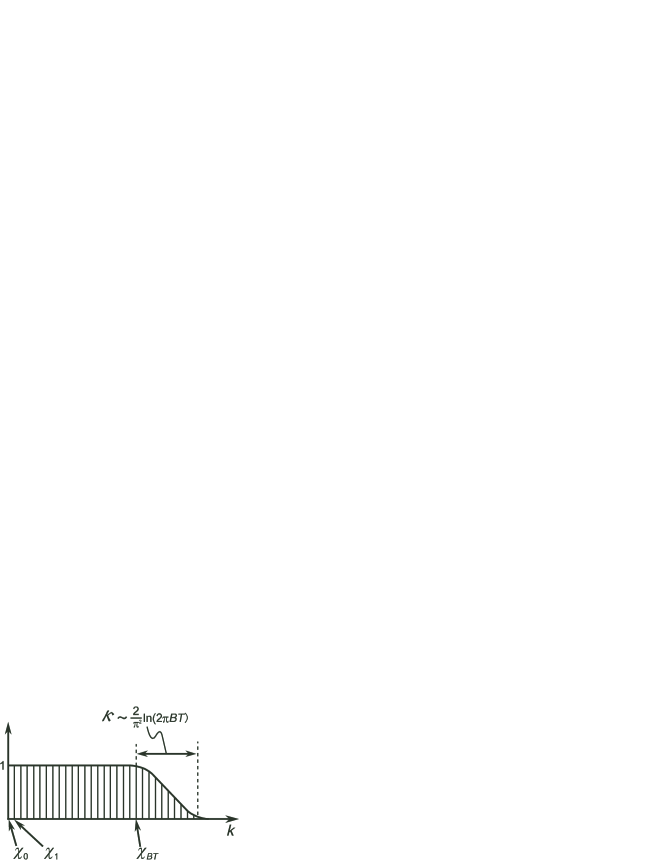
Figure 5: Eigenvalu spectrum of $\chi_{k}(c)$ for $BT\gg 1$.

In the case of $BT\ll 1$, on the other hand, the 0th eigenvalue scales as $\chi_{0}(c)\sim BT$ and $\chi_{0}(c)\gg\chi_{k}(c)$ for $k\geq 1$, namely, only the 0th mode contributes with the weight $BT$. The first few eigenvalues $\chi_{k}(c)$ for several values of $BT$ are given in Table 1, which is borrowed from Zhu and Caves Zhu_Caves90 . This means that in Eq. (108), $\mathrm{w}^{\mathrm{S}}\sim BT\ll 1$ and $\mathrm{w}^{\mathrm{V}}\sim 1-BT\approx 1$. The second term in Eq. (108) represents the vacuum fluctuations due to the modes outside the squeezing bandwidth. Actually if one measures the squeezed state in an interval much shorter than $\sim B^{-1}$, one will observe wide range of frequency modes in vacuum states. When this term becomes dominant, the squeezing characteristics cannot be observed clearly, being covered by the vacuum fluctuation noise. This could be a serious restriction on optimization of the mode matching. In the next subsection we consider a scheme to remove this restriction by using an electrical low pass filter.

$k$	$BT=0.1$	$BT=0.5$	$BT=1.0$	$BT=3.0$
0	0.09973	0.46780	0.78340	0.99890
1	0.00027	0.03183	0.20502	0.96869
2	0.00000	0.00037	0.01136	0.73284
3		0.00000	0.00021	0.26248
4			0.00000	0.03478
5				0.00221
6				0.00009

Table 1: The first few eigenvalues $\chi_{k}(c)$ for several values of $BT$.

VI.2 LO matched mode measured by homodyne detector with a finite bandwidth

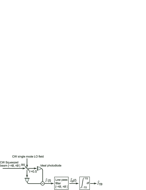
Figure 6: Time-integrated homodyne detection with a low pass filter in a CW setting.

Figure 7: CW scheme of the non-Gaussian operation by photon subtraction with the on/off detector.

Let us consider a scheme shown in Fig. 6, where an electrical low pass filter is inserted into the scheme of Fig. 4. The intantaneous homodyne current Eq. (33) is first filtered by the low pass filter with the same bandwidth $B$ matched to the squeezing spectrum, and is then integrated over the interval $[-T/2,T/2]$. The filtered current can be simply represented as

$$\hat{I}_{B}(t)=\frac{\alpha^{\mathrm{L}}}{4\pi^{2}}\int_{-\pi B}^{\pi B}d\Omega\left[\hat{A}(\Omega)e^{-i\phi}+\hat{A}^{\dagger}(-\Omega)e^{i\phi}\right]e^{-i\Omega t}.$$ (111)

It is finally time-integrated over the interval $T$

$$\hat{I}_{TB}=\frac{\alpha^{\mathrm{L}}}{2\pi}\int_{-\pi B}^{\pi B}d\Omega\left[\hat{A}(\Omega)e^{-i\phi}+\hat{A}^{\dagger}(\Omega)e^{i\phi}\right]\frac{\sin\frac{\Omega T}{2}}{\pi\Omega}.$$ (112)

In this equation the field $\hat{A}(\Omega)$ is band-limited and hence can be expanded in terms of $\hat{A}_{k}$ by Eq. (29), resulting in

$$\hat{I}_{TB}=\frac{\alpha^{\mathrm{L}}}{{\sqrt{2}}\pi}\sum_{k=0}^{\infty}\hat{X}_{k}^{\mathrm{S}}\int_{-\pi B}^{\pi B}d\Omega\Phi_{k}(c,\Omega)\frac{\sin\frac{\Omega T}{2}}{\pi\Omega},$$ (113)

where the definition Eq. (44) is used by setting $\phi=0$. By using the relation Eq. (16), the above equation is rewritten as

$$\hat{I}_{TB}=\frac{\alpha^{\mathrm{L}}}{{\sqrt{2}}\pi}\sum_{k=0}^{\infty}\hat{X}_{k}^{\mathrm{S}}\chi_{k}(c)\Phi_{k}(c,0).$$ (114)

So in this case the observed LO matched mode is specified only by the quadrature operator on the Hilbert space $\cal H^{\mathrm{S}}$

$$\tilde{X}_{0}=\sum_{k=0}^{\infty}\epsilon_{k}\hat{X}_{k}^{\mathrm{S}},$$ (115)

where

$$\epsilon_{k}=\frac{\chi_{k}(c)\Phi_{k}(c,0)}{\sqrt{\displaystyle\sum_{k=0}^{\infty}\chi_{k}(c)^{2}\Phi_{k}(c,0)^{2}}},$$ (116)

which is non-zero only for even $k$, because of Eq. (106) and Eq. (107). The observed variance Eq. (108) then reduces to

$$\sigma_{-}^{2}=e^{-2\gamma},$$ (117)

which is independent of the integration time $T$. Thus in this case one can observe the intrinsic characteristics of the squeeezing regardless of the choice of $T$. This is essential for achieving stringent mode matching in the regime of $BT\ll 1$.

VI.3 Numerical examples and mode matching design chart

After all, we consider the CW scheme depicted in Fig. 7. The CW squeezed beam is splitted with reflectance $1-\tau=0.1$. The 10% of the squeezed beam is tapped off, and is guided into the on/off detector, which is opened for the time duration $[-T/2,T/2]$ by electrical gating. This defines the discrete events in the time domain. The average interval between the successive trigger events (“on” counts) is assumed to be long enough compared with $T$. In the homodyne detector, the CW signal beam is combined with the CW single mode LO field, producing the CW current $\hat{I}(t)$, and this is filtered by the low pass filter matched to the squeezing bandwidth. Only when the “on” signal is sent from the trigger channel, the filtered current $\hat{I}_{B}(t)$ is integrated over $[-T/2,T/2]$ synchronized with the gating signal. The quadrature operator of Eq. (115) based on the integrated current $\hat{I}_{TB}$ is used to construct the Wigner function of the conditional statistics.

As a typical model of squeezing, we assume $\gamma=0.35$ (3 dB squeezing) and $B=10$ MHz. The net detection efficiency of the on/off detector $\eta$, which appears in the effective quantum efficiency for mode $k$ as $\eta_{k}=\eta\chi_{k}(c)$, is determined by the total coupling efficiency of photons through filters and couplers to the photondetector, and the intrinsic quantum efficiency of the photondetector. So this can be a small value something like $<$0.5. The mean number of dark counts $\nu_{k}$ for mode $k$ can be converted into the dark count rate $n$ [counts/s] by $\sum_{k}\nu_{k}=nT$. We vary this $n$ [counts/s] to evaluate the dark count effect.

In Figs. 8 trough 11, we show the values of the Wigner function at the phase space origin as a function of the dark count rate $n$ [counts/s] for several values of $BT$. The mode weights $\{\chi_{k}(c)\}$ are given in Table 1. $BT=0$ means the single mode case with perfect mode matching. Figs. 8, 9, 10, and 11 corresponds to the different detection efficiencies of the on/off detector, $\eta=0.01$, 0.1, 0.7 and 1. From these figures, we can know the threshold for the on/off detector dark counts below which one can expect to observe the negative dip of the Wigner function, which is a sign of the non-classicality of the non-Gaussian output state. As the detection efficiency $\eta$ becomes smaller, the threshold dark count for the negative dip also gets smaller.

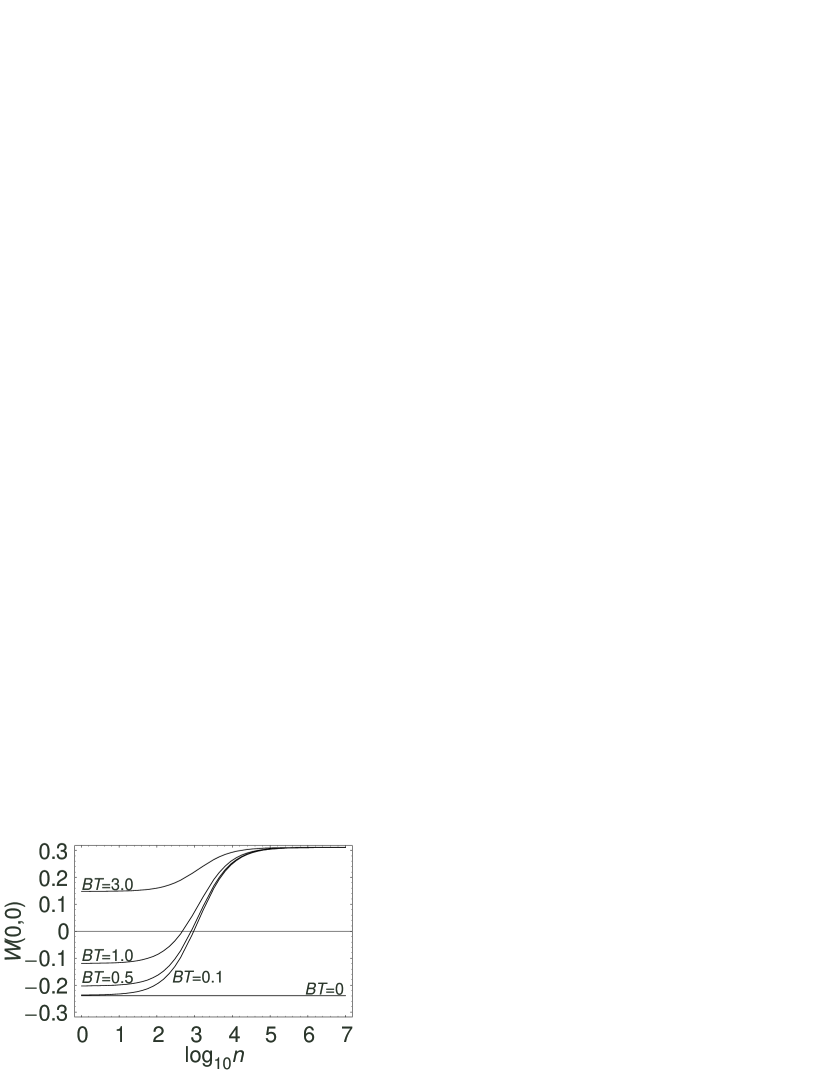
Figure 8: Values of the Wigner functions at the origin of the phase-space, versus the dark count rate $n$ [counts/s], under the condition of 3 dB squeezing, $\eta=0.01$, and $\tau=0.9$

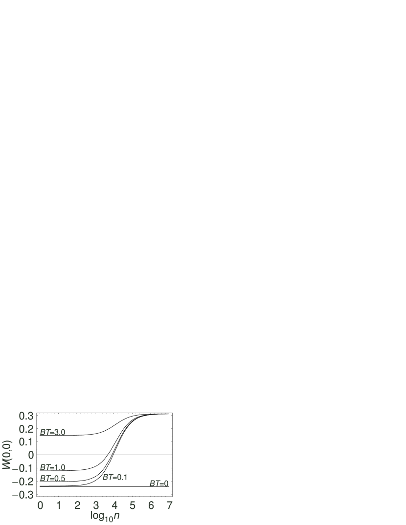
Figure 9: Values of the Wigner functions at the origin of the phase-space, versus the dark count rate $n$ [counts/s], under the condition of 3 dB squeezing, $\eta=0.1$, and $\tau=0.9$

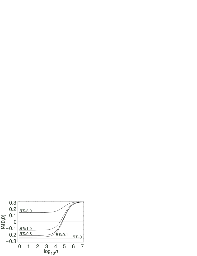
Figure 10: Values of the Wigner functions at the origin of the phase-space, versus the dark count rate $n$ [counts/s], under the condition of 3 dB squeezing, $\eta=0.7$, and $\tau=0.9$

Figure 11: Values of the Wigner functions at the origin of the phase-space, versus the dark count rate $n$ [counts/s], under the condition of 3 dB squeezing, $\eta=1$, and $\tau=0.9$

For larger values of $BT$, the mismatch between the LO matched mode and the photon mode observed by the on/off detector becomes more serious. For $BT=3.0$, one could not attain the negative dip of the Wigner function even with the ideal on/off detector. Actually, in the case of $BT\gg 1$, the first ${\cal{N}}\sim BT$ modes have eigenvalues $\chi_{k}(c)$ near 1, and then the eigenvalues fall from near 1 to near 0 rapidly as $k$ increases, as shown in Fig. 5. All the first ${\cal{N}}\sim BT$ modes cause trigger signals at the on/off detector, which makes the conditional state at the signal port a highly mixed state, because the on/off detector cannot discriminate which mode a photon comes from. On the other hand, the homodyne detector sees only the LO matched mode, which is a particular combination of the first ${\cal{N}}\sim BT$ modes, and provides the homodyne statistics for the single mode quadrature operator defined by Eq. (115).

In the case of $BT\ll 1$, on the other hand, $\chi_{0}(c)\sim BT$ and $\chi_{0}(c)\gg\chi_{k}(c)$ for $k\geq 1$. So only the 0th mode is dominant both in the trigger channel and the homodyne detector: more precisely, the POVM element for the “on” signal $\hat{\Pi}_{\mathrm{on}}^{\mathrm{B}}(\bm{\eta},\bm{\nu})$ in Eq. (IV) and the quadrature eigenstate $\left|x\right)$ on the Hibert space ${\cal H}^{\mathrm{L}}$ describing the homodyne detector (see the text from Eq. (59) to Eq. (75)). If one further takes a small reflectance for the tapping beam splitter, making the probability of detecting more than two photons at the on/off detector very small, then the trigger photons are projected onto an almost pure single photon state. The homodyne detector measures the same pure state with almost perfect efficiency, attaining the best mode matching. The small tapping fraction, combined with a small value of $\chi_{0}(c)\sim BT$, means a small efficiency for the on/off detector. This is usually unwanted, but in the present context this simply results in the reduction of the number of selected events. If the number of true trigger events can be kept larger than the dark counts, this reduction would be an acceptable sacriface to attain better mode matching.

One should note that it is essential to filter the homodyne current by the low pass filter matched to the squeezing bandwidth $B$ before integrating over the interval $[-T/2,T/2]$. If the ideal homodyne detector with wider enough bandwidth than $B$ would be used, the vacuum fluctuation would also become dominant in the homodyne statistics especially for shorter $T$. This component does not have any mode overlap with the trigger photons at the on/off detector, and would degrade the mode matching quality.

Figs. 12, 13, and 14 represent the Wigner function distributions at the point of dark count $n=500$ [counts/s] in Fig. 9 ($\eta=0.1$) for the three kinds of $BT=$ 0.0, 0.5, and 1.0, where one can still expect the negative dip.

Figure 12: Wigner function distribution for $BT=0$, i.e. the ideal single mode case, at the point of dark count $n=500$ [counts/s] in Fig. 9 (3 dB squeezing, $\tau=0.9$, $\eta=0.1$)

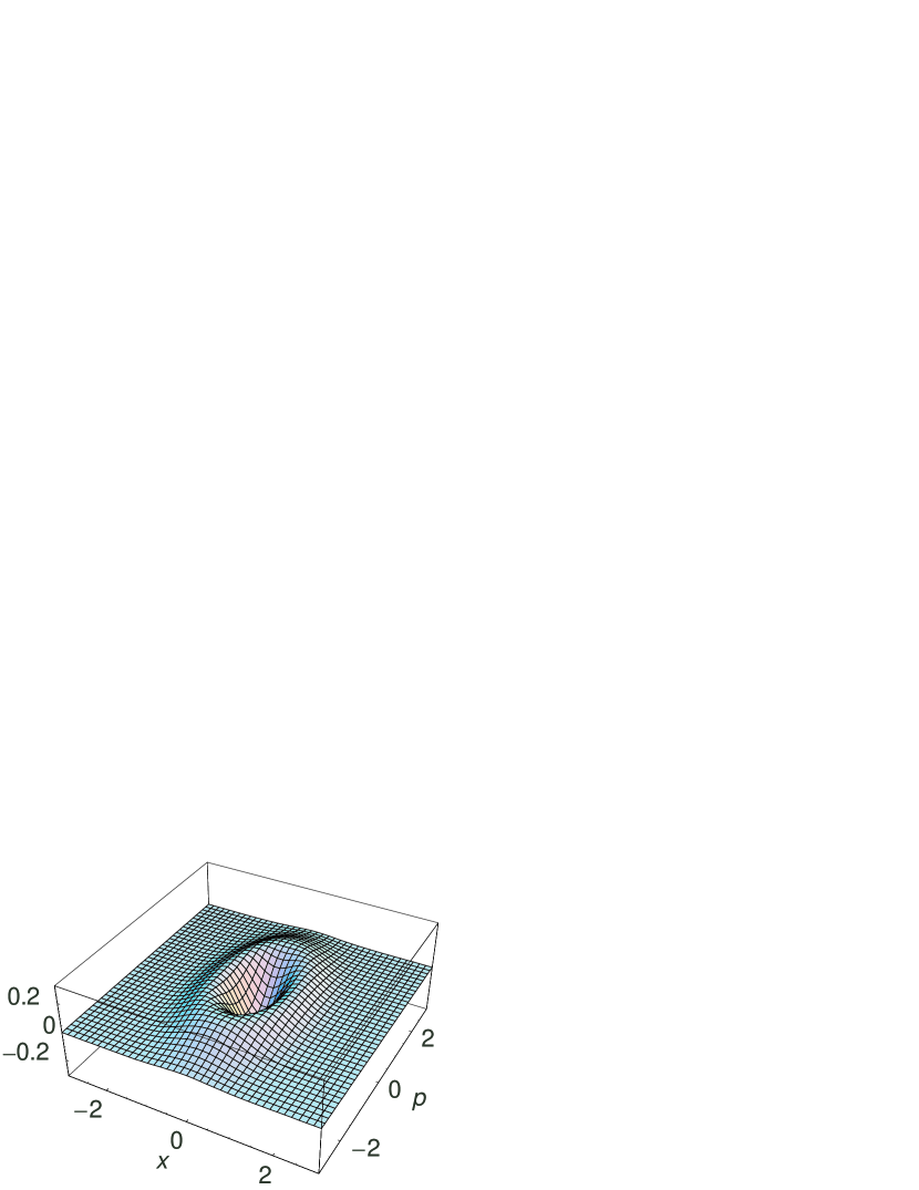
Figure 13: Wigner function distribution for $BT=0.5$ at the point of dark count $n=500$ [counts/s] in Fig. 9 (3 dB squeezing, $\tau=0.9$, $\eta=0.1$)

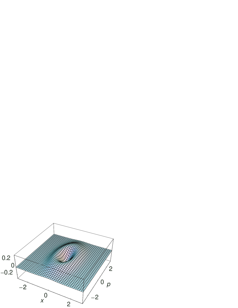
Figure 14: Wigner function distribution for $BT=1.0$ at the point of dark count $n=500$ [counts/s] in Fig. 9 (3 dB squeezing, $\tau=0.9$, $\eta=0.1$)

VII Pulsed scheme

In this section we consider a scheme using Fourier-transform limited short pulses. A pulse width of the fundamental field (LO field) is typically 1 ps or shorter, so that the spectral width is about 1  THz or wider. The pump field is the frequency-doubled LO with almost the same spectral width. A nonlinear crystal is pumped in a traveling-wave configuration in a single path. Then unlike the CW configuration, the down-converted (squeezed) field has generally different mode properties from the ones of the pump and the LO fields. The finiteness of the nonlinear crystal broadens the phase-matching condition, producing a wider bandwidth of squeezing than that of the LO. The group velocity mismatch increases the pulse duration, and makes the field apart from the Fourier-transform limit. The group velocity dispersion induces a frequency charp. These discrepancies between the signal and the LO field properties degrade the degree of mode matching. In order to overcome this problem, the usage of optical filters with narrow bandwidth in the trigger channel was enphasized in Ou97QSemiclOpt ; Grosshans01 ; Aichele Lvovsky Schiller 02EurPhysJD ; Viciani Zavatta Bellini 04PRA . In these works, a biphoton source state

$$\left|\rho\right\rangle_{\mathrm{AB}}=\left|0\right\rangle_{\mathrm{A}}\left|0\right\rangle_{\mathrm{B}}-i\int d^{3}kd\omega d^{3}k^{\prime}d\omega^{\prime}$$

$$\times\Psi(\mathbf{k},\omega,\mathbf{k}^{\prime},\omega^{\prime})\left|\mathbf{k},\omega\right\rangle_{\mathrm{A}}\left|\mathbf{k}^{\prime},\omega^{\prime}\right\rangle_{\mathrm{B}}$$ (118)

is assumed. Here $\left|\mathbf{k},\omega\right\rangle_{\mathrm{j}}$ means the single photon state with momentum $\mathbf{k}$ and frequency $\omega$ in path j (=A, B), and the function $\Psi(\mathbf{k},\omega,\mathbf{k}^{\prime},\omega^{\prime})$ characterizes the correlation properties of the biphoton state. Since we are concerned here with frequency mode matching, we shall suppress the momentum representation. The trigger photon at path B is selected by frequency filters, and is then detected by an ideal photon counter. When the photon counter clicks, the trigger state is projected onto a POVM element

$$\hat{\Pi}_{\mathrm{on}}=\int d\omega F(\omega)\left|\omega\right\rangle_{\mathrm{B}}\left\langle\omega\right|,$$ (119)

where $F(\omega)$ includes filter characteristics and the effective quantum efficiency of the photon counter for each frequency mode. The conditional signal state at path A is then given by

$$\hat{\rho}_{\mathrm{A}}=\frac{\mathrm{Tr}_{\mathrm{B}}\left(\hat{\Pi}_{\mathrm{on}}\left|\rho\right\rangle_{\mathrm{(AB)}}\left\langle\rho\right|\right)}{\mathrm{Tr}_{\mathrm{AB}}\left(\hat{\Pi}_{\mathrm{on}}\left|\rho\right\rangle_{\mathrm{(AB)}}\left\langle\rho\right|\right)}.$$ (120)

In Aichele Lvovsky Schiller 02EurPhysJD , the correlation function

$$\Gamma(\omega,\omega^{\prime})=\mathrm{Tr}\left[\hat{\rho}_{\mathrm{A}}\hat{a}^{\dagger}(\omega)\hat{a}(\omega)\right],$$ (121)

and the modal purity

$$P=\mathrm{Tr}\left(\hat{\rho}_{\mathrm{A}}^{2}\right),$$ (122)

were introduced, and a measure of mode matching $M$ is defined using the correlation function. The quality of mode matching was analyzed in terms of these $M$ and $P$. However, it has been unclear how to obtain explicit expressions of the quantum states when these quantities are given.

Our interest here is a more direct quantity than $M$ and $P$, that is, the Wigner function of $\hat{\rho}_{\mathrm{A}}$ finally obtained by the homodyne detection. In addition, the source state is not the photon pair but the wideband squeezed state, which is beyond the first order perturbation theory. The source state is a flat band squeezed state $\left|\mathbf{r}_{0}\right\rangle=\hat{S}_{0}\left|\mathbf{0}\right\rangle$

$$\hat{S}_{0}=\mathrm{exp}\Biggl{(}\frac{\gamma}{4\pi}\int_{-\pi B_{\mathrm{S}}}^{\pi B_{\mathrm{S}}}d\Omega\biggl{[}\hat{A}(\Omega)\hat{A}(-\Omega)$$

$$-\hat{A}^{\dagger}(\Omega)\hat{A}^{\dagger}(-\Omega)\biggr{]}\Biggr{)},$$ (123)

where the squeezing bandwidth $B_{\mathrm{S}}$ is usually much wider than that of the LO $B$, i.e. $B_{\mathrm{S}}\gg B$. Here we have omitted the group velocity dispersion and mismatch, because this simply causes slight quantitative modification for the filtered state, and is not essential in considering the frequency mode matching here.

We should first derive the quadrature eigenstate $\left|x\right)$ to describe the POVM of the homodyne detector. For simplicity, we assume the LO field with a flat band spectrum over the bandwidth $B$

$$\hat{A}^{\mathrm{L}}(\Omega)=\left\{\begin{array}[]{ll}\alpha^{\mathrm{L}}e^{i\phi}&\quad(|\Omega|\leq\pi B),\\ 0&\quad\mathrm{otherwise}.\end{array}\right.$$ (124)

The instantaneous homodyne current is then given by

$$\hat{I}(t)=\frac{1}{2\pi}\int_{-\infty}^{\infty}d\Omega\hat{I}(\Omega)e^{-i\Omega t}$$ (125)

with

$$\hat{I}(\Omega) = \frac{1}{2\pi}\int_{-\infty}^{\infty}d\Omega^{\prime}\biggl{[}\hat{A}^{\mathrm{L\dagger}}(\Omega^{\prime})\hat{A}(\Omega+\Omega^{\prime})$$ (126)

$$+\hat{A}^{\dagger}(-\Omega+\Omega^{\prime})\hat{A}^{\mathrm{L}}(\Omega^{\prime})\biggr{]}$$

$$= \frac{\alpha^{\mathrm{L}}}{2\pi}\int_{-\pi B}^{\pi B}d\Omega^{\prime}\biggl{[}\hat{A}(\Omega+\Omega^{\prime})e^{-i\phi}$$

$$+\hat{A}^{\dagger}(-\Omega+\Omega^{\prime})e^{i\phi}\biggr{]}.$$

Note that the field operator at the signal port $\hat{A}(\Omega)$ itself is not band-limited. If the homodyne detector would have the infinite bandwidth, then the instantaneous current $\hat{I}(t)$ provides the final observable. In practice, however, this is not the case. Rather, the effective bandwidth of the homodyne detector including the photodiodes and the electronics, $B_{\mathrm{H}}$ is much narrower than that of the LO. Typically, $B_{\mathrm{H}}$ is a few hundred MHz at most while $B\geq$1 THz. So one actually measures the low frequency components within the homodyne detector bandwidth. We shall approximately model it as

$$\hat{I}_{B_{\mathrm{H}}}(t) = \frac{1}{2\pi}\int_{-\pi B_{\mathrm{H}}}^{\pi B_{\mathrm{H}}}d\Omega\hat{I}(\Omega)e^{-i\Omega t}$$ (127)

$$= \frac{\alpha^{\mathrm{L}}}{4\pi^{2}}\int_{-\pi B_{\mathrm{H}}}^{\pi B_{\mathrm{H}}}d\Omega e^{-i\Omega t}\int_{-\pi B}^{\pi B}d\Omega^{\prime}$$

$$\times\biggl{[}\hat{A}(\Omega+\Omega^{\prime})e^{-i\phi}+\hat{A}^{\dagger}(-\Omega+\Omega^{\prime})e^{i\phi}\biggr{]}$$

$$\approx \frac{\alpha^{\mathrm{L}}}{2\pi}\cdot\frac{\sin\pi B_{\mathrm{H}}t}{\pi t}$$

$$\times\int_{-\pi B}^{\pi B}d\Omega\biggl{[}\hat{A}(\Omega)e^{-i\phi}+\hat{A}^{\dagger}(\Omega)e^{i\phi}\biggr{]}.$$

The field operator $\hat{A}(\Omega)$ is now band-limited to $B$, and can be expanded by the discrete set of the prolate spheroidal wave function basis. Using the formula in Section II, we have

$$\hat{I}_{B_{\mathrm{H}}}(t)\approx{\sqrt{2}}\alpha^{\mathrm{L}}\frac{\sin\pi B_{\mathrm{H}}t}{\pi t}\sum_{k=0}^{\infty}\hat{X}_{k}^{\mathrm{S}}(\phi)\Psi_{k}(c,0),$$ (128)

where the quadrature operator $\hat{X}_{k}^{\mathrm{S}}(\phi)$ is defined by Eq. (44). The time dependent factor means that a short optical pulse with a duration $T\sim B^{-1}$, say $\sim 1$  ps, is converted into an electrical pulse with a duration $T_{\mathrm{H}}\sim B_{\mathrm{H}}^{-1}\sim 0.1$  ns. As seen from this equation it is sufficient to sample the peak value of the electrical pulse

$$\hat{I}_{B_{\mathrm{H}}}(0)\approx{\sqrt{2}}\alpha^{\mathrm{L}}B_{\mathrm{H}}\sum_{k=0}^{\infty}\hat{X}_{k}^{\mathrm{S}}(\phi)\Psi_{k}(c,0),$$ (129)

for the quadrature values. The final observable is then given by

$$\tilde{X}_{0}=\sum_{k=0}^{\infty}\epsilon_{k}\hat{X}_{k}^{\mathrm{S}},$$ (130)

where

$$\epsilon_{k} = \frac{\Psi_{k}(c,0)}{\sqrt{\displaystyle\sum_{k=0}^{\infty}|\Psi_{k}(c,0)|^{2}}},$$ (131)

$$= \frac{(-1)^{k}\sqrt{(2k+1)\chi_{k}(c)}P_{k}(c,0)}{\sqrt{\displaystyle\sum_{k=0}^{\infty}(2k+1)\chi_{k}(c)P_{k}(c,0)^{2}}},$$

which is non-zero only for even $k$. The POVM of the pulsed homodyne detector is represented by the projection $\left|x\right)\left(x\right|$ onto the eigenstates of $\tilde{X}_{0}$, tracing out all the other modes.

If the trigger beam is projected onto the single photon state $\left|1\right)$ on the subspace $\cal H^{\mathrm{L}}$ spanned by $\left|x\right)$, the ideal photon-subtracted non-Gaussian state would be obtained. Toward this limit, the trigger beam must be band-limited to $B$, since the homodyne observable consists of the frequency modes within the LO bandwidth $|\Omega|\leq\pi B$. It can be made by interference band pass filters typically with 0.1-1 nm spectral width. The band-limited trigger beam is finally detected by the on/off detector. The on/off detector responds much more slowly, say in a scale of $T_{\mathrm{D}}\gtrsim 300$ ps, than the pulse width $T\lesssim 1$ ps. But if we assume that the average interval between “on” signals is still much longer than this $T_{\mathrm{D}}$, and also that the photoelectric conversion does not significatly destroy the Fourier-transform limited pulses. Then the on/off detector can be represented by the state basis of the prolate spheroidal wave functions for the $BT$, as described in Section IV.

The photon subtracted non-Gaussian state at path A is given by

$$\hat{\rho}_{\mathrm{A}}=\frac{{\rm\,Tr}\,_{\mathrm{B}}\left[\left|\rho\right\rangle_{\mathrm{(AB)}}\left\langle\rho\right|\hat{I}^{\mathrm{A}}\otimes\hat{\Pi}_{\mathrm{on}}^{\mathrm{B}}(\bm{\eta},\bm{\nu})\right]}{{\rm\,Tr}\,_{\mathrm{AB}}\left[\left|\rho\right\rangle_{\mathrm{(AB)}}\left\langle\rho\right|\hat{I}^{\mathrm{A}}\otimes\hat{\Pi}_{\mathrm{on}}^{\mathrm{B}}(\bm{\eta},\bm{\nu})\right]}.$$ (132)

Since $\hat{\Pi}_{\mathrm{on}}^{\mathrm{B}}$ detects only the modes in $|\Omega|\leq\pi B$, and these modes are not quantum correlated with the ones outside of it, the state $\left|\rho\right\rangle_{\mathrm{AB}}$ can be regarded as the beam splitted state from the squeezed state $\left|\mathbf{r}\right\rangle=\hat{S}\left|\mathbf{0}\right\rangle$ where

$$\hat{S} = \mathrm{exp}\Biggl{(}\frac{\gamma}{4\pi}\int_{-\pi B}^{\pi B}d\Omega\biggl{[}\hat{A}(\Omega)\hat{A}(-\Omega)$$ (133)

$$-\hat{A}^{\dagger}(\Omega)\hat{A}^{\dagger}(-\Omega)\biggr{]}\Biggr{)}$$

$$= \bigotimes_{k=0}^{\infty}\mathrm{exp}\left[\frac{r_{k}}{2}\left(\hat{A}_{k}^{2}-\hat{A}_{k}^{\dagger 2}\right)\right],$$

instead of the squeezed state $\left|\mathbf{r}_{0}\right\rangle=\hat{S}_{0}\left|\mathbf{0}\right\rangle$ of Eq. (VII). Thus the photon subtracted state $\hat{\rho}_{\mathrm{A}}$ is represented in terms of $\{\hat{A}_{k}\}$ or $\{\hat{X}_{k}^{\mathrm{S}}\}$ and its eigenstates $\{\left|x_{k}^{\mathrm{S}}\right\rangle\}$. Its Wigner function can then be calculated by the formulus (94). The mode matching consideration proceeds just as the CW case in Section VI.3. Good mode matching is achieved when the weight coefficient $\epsilon_{0}$ dominates the other ones $\epsilon_{1},\epsilon_{2},...$. This can be made by setting the valuse $BT$ as small as possible. In the pulsed scheme, however, the $T$ is automatically set by the laser pulse width. It is actually impossible at present to realize a shorter measurement interval because electrical gating cannot reach such a time scale. Therefore the value of $BT$ is lower bounded by the Fourier-transform limit, which is about $BT\approx 1$ or slightly less. Then a few lower modes can contribute, as shown in Table 1. This is already enough to observe the negative dip in the Wigner function, provided that mode matching with respect to the other degrees of freedom can be made perfect.

In experimental practice of the pulsed scheme, however, it is generally not easy to realize a high quality spatiotemporal mode matching unlike the CW scheme based on cavity OPO systems. For meaningful numerical evaluations, consideration on imperfections due to the spatial mode mismatch should be involved. But this is beyond the scope of this paper.

VIII Conclusion

We have developed a theory to design the frequency mode matching in the photon-subtracting operation by the on/off-type photon detector on the wideband squeezed state. It is essential to represent the POVMs of the on/off photon detection and the homodyne detection in terms of an appropriate basis under time- and band-limitation on the fields. Such a set is based on the prolate spheroidal wave functions which are complete and orthonormal under the time- and band-limitation. The POVMs thus represented define the measured modes, and hence the quantum states of the trigger photons and the conditionally selected homodyne events. The mode matching is pursued for those quantum states.

Our theory has been applied to the CW and pulsed schemes. In both schemes, the desired condition for good frequency mode mathching is $BT\lesssim 1$. In the previous works Ou97QSemiclOpt ; Grosshans01 ; Aichele Lvovsky Schiller 02EurPhysJD ; Viciani Zavatta Bellini 04PRA , only narrowband spectral filtering is emphasized. But the quantity to be set smaller is the product $BT$. In addition, the modes of interest are not the ones specified by the plane wave basis  Ou97QSemiclOpt ; Grosshans01 ; Aichele Lvovsky Schiller 02EurPhysJD ; Viciani Zavatta Bellini 04PRA but rather the ones specified by the prolate spheroidal wave functions under the time- and band-limitation. In the regime $BT\lesssim 1$, the discreteness of modes becomes prominant, and only a few lower modes of the prolate spheroidal wave functions are excited. For $BT\lesssim 0.5$, only the 0th mode becomes dominant with the mode weight $\chi_{0}(c)\sim BT$ as seen in Table 1. Then the trigger channel selects a pure single photon state in mode 0 if one takes a small reflectance $1-\tau$ of the tapping beam splitter, and could suppress dark counts. The homodyne detector measures the same pure state with almost perfect efficiency, attaining the ideal mode matching.

The increase of $BT$ and the dark counts makes the conditional state more mixed over many modes of $k$, while the homodyne detector still projects the conditional state onto a pure eigenstate of the LO matched quadrature operator, which is a particular combination of the first ${\cal{N}}\sim BT$ modes. Then the non-classical effect in homodyne statistics will be smeared out.

In the CW scheme where all the beams are CW, such as based on cavity OPO systems, the effective bandwidth can be set in a range of $B\approx 10$  MHz by using an appropriate set of filtering cavities placed in fromt of the on/off detector, and an electrical low pass filter in the homodyne detector spectrally matched to the squeezing. Then the time duration $T$ for the desired condition $BT\lesssim 1$ is of order of sub $\mu$s, which can readily be achieved by current electrical gating. A smaller $T$ allows one more stringent frequency mode matching. The lower bound for $T$ may be set by the temporal resolution of the homodyne detector, which is currently of order of a few ns. So the frequency mode matching in a regime $BT\lesssim 0.1$ can be attained in principle. The spatial mode matching can also be fulfilled by carefully locking the cavities. The temporal mode matching in the sub $\mu$s is not a problem. Then the numerical results presented in Section  VI.3 can be practical design charts. One may expect to realize the negative dip of the Wigner function at the phase space origin for practical experiental parameters. All in all, the CW scheme will provide a good test-bed for the non-Gaussian operations based on photon counting and homodyning.

In the pulsed scheme, the time duration $T$ is automatically set by the laser pulse width, typically ps order. The band limitation comes from the LO bandwidth, $\approx 1$ THz, corresponding to the Fourier-transform limit $0.5\lesssim BT\lesssim 1$. The time response of the homodyne detector is much slower than the LO pulse width. Then by sampling the peak value of the homodyne current pulse, one finally observes the quadrature composed linearly of a few lower modes of $k$. This makes the situation very similar to the CW case, and the numerical examples in Section VI.3 can apply. So the frequency mode matching needed for observing the negative dip of the Wigner function will be possible. In practical experiments, such as ref. Wenger04 , however, the observed dip of the Wigner function is still positive. This may be partly attributed to the imperfect spatial mode mathing between the trigger photons and the LO field. It is generally more difficult, compared with the cavity CW scheme, to control the wave front of the pulsed field, and to spatially match the relevant modes.

Now we would like to mention the relation between our result and the one obtained by Grosshans and Grangier Grosshans01 . They predicted the lower degree of mode matching for the CW scheme than for the pulsed one. This seems to be contradict with our result. In Grosshans01 , however, some points are missing. Firstly, the POVM element in the trigger channel was modeled by a projection onto a pure state

$$\hat{\Pi}_{\mathrm{on}}=\int_{-\pi B}^{\pi B}d\Omega\left|\Omega\right\rangle\int_{-\pi B}^{\pi B}d\Omega^{\prime}\left\langle\Omega^{\prime}\right|,$$ (134)

instead of Eq. (119). But photon counters cannnot be sensitive to the relative phases of different frequency components. So the modeling by the above equation is unlikely, as also pointed out by Aichele et al. Aichele Lvovsky Schiller 02EurPhysJD . Secondly, the parameter $X=\delta\omega_{i}\delta T/2\pi$ in Grosshans01 , which corresponds to $BT$ in this paper, could not be arbitrary small for the Fourier-transform limited pulses. According to these points, the degree of the mode overlap $\eta_{\mathrm{eff}}(X)$ should be reconsidered in the pulsed regime. Finally, the analysis on the “chopped” CW scheme did not take the time- and band-limitation into acount. In Grosshans01 , the single parameter

$$\eta_{\mathrm{eff}}(BT)=\frac{1}{BT}\left|\int_{-\pi B}^{\pi B}d\Omega\frac{\sin\frac{\Omega T}{2}}{\pi\Omega}\right|^{2},$$ (135)

was used for quantifying the degree of mode matching. But this cannot be sufficient for treating the time- and band-limited signals. More precisely the mode matching must be characterized by the set of mode weights

$$\int_{-\pi B}^{\pi B}d\Omega\Phi_{k}(c,\Omega)\frac{\sin\frac{\Omega T}{2}}{\pi\Omega}=\chi_{k}(c)\Phi_{k}(c,0).$$ (136)

Therefore the upper bound $\eta_{\mathrm{eff}}(X)\leq 0.825$ for the CW scheme derived in Grosshans01 will not be the true limit. Rather the more stringent matching will be possible as shown in this paper.

Concerning to the CW scheme, we should also mention the effect of chopping the beams for the duration $T$. The scheme in this paper is to use the CW single-mode LO and then to integrate the CW homodyne current over $T$. This is equivalent to using the chopped LO with the duration $T$, if the detector bandwidth is infinite. Remember that the homodyne detector with the infinite bandwidth suffers from the vacuum fluctuations outside the squeezing bandwidth for shorter $T$. So we have considered installing the matched low pass filter. In such a band-limited case, using the chopped LO will not generally be equivalent to integrating the CW current over $T$ afterward. In fact, chopping the CW single-mode LO modifies its spectrum from $\delta(\Omega)$ to $\sin(\Omega T/2)/\pi\Omega$. Then the homodyne current is also modulated accordingly, and is then filtered. According to the present analysis, the use of the chopped LO does not seem to bring any particular merit. Therefore it will be enough to simply use the CW single-mode LO, and to electrically gate the on/of detetor to define the events in the time domain.

*

Appendix A Prolate Spheroidal Wave Functions

In this appendix basic properties of the prolate spheroidal wave functions are sumarized for reader’s convenience. The differential equation

$$(1-x^{2})\frac{d^{2}u}{dx^{2}}-2x\frac{du}{dx}+(\mu-c^{2}x^{2})u=0,$$ (137)

has continuous solutions in the closed set $x$ interval $[-1,1]$ only for certain discrete real positive values,

$$0<\mu_{0}(c)<\mu_{1}(c)<\mu_{2}(c)<\cdots.$$ (138)

Corresponding to each eigenvalue $\mu_{k}(c)$, there is a unique solution $S_{0k}(c,x)$ such that it reduces to the $k$th Legendre polynomial $P_{k}(x)$ uniformly in $[-1,1]$ as $c\rightarrow 0$. The functions $S_{0k}(c,x)$ are called the angular prolate spheroidal wave functions. They are real for real $x$, continuous functions of $c$ for $c\geq 0$, and orthogonal in $(-1,1)$. $S_{0k}(c,x)$ has exactly $k$ zeros in $(-1,1)$, and even and odd according as $k$ is even and odd.

Alternatively $S_{0k}(c,x)$ is also a solution of the integral equation

$$\chi_{k}(c)S_{0k}(c,x)=\int_{-1}^{1}dy\frac{\sin c(x-y)}{\pi(x-y)}S_{0k}(c,y),\quad|x|\leq 1.$$ (139)

The eigenvalues $\chi_{k}(c)$ are expressed by using a second set of solution $R_{0k}^{(1)}(c,x)$ for (137), called the radial prolate spheroidal wave functions, as

$$\chi_{k}(c)=\frac{2c}{\pi}\left[R_{0k}^{(1)}(c,1)\right]^{2}.$$ (140)

$R_{0k}^{(1)}(c,x)$ differ from $S_{0k}(c,x)$ only by a real scale factor.

From Eq. (139), we have

$$\chi_{k}(c)\Psi_{k}(c,t)=\int_{-T/2}^{T/2}dt^{\prime}\frac{\sin\pi B(t-t^{\prime})}{\pi(t-t^{\prime})}\Psi_{k}(c,t^{\prime}),$$ (141)

and

$$\chi_{k}(c)\Phi_{k}(c,\Omega)=\int_{-\pi B}^{\pi B}d\Omega^{\prime}\frac{\sin\frac{(\Omega-\Omega^{\prime})T}{2}}{\pi(\Omega-\Omega^{\prime})}\Phi_{k}(c,\Omega^{\prime}).$$ (142)

The orthogonal condition of Eq. (25) can be derived by using Eq. (141) and the orthonormal condition

$$\int_{-\infty}^{\infty}dt\Psi_{k}(c,t)\Psi_{l}(c,t)=\delta_{kl}.$$ (143)

Another important relation is

$$2i^{k}R_{0k}^{(1)}(c,1)S_{0k}(c,x)=\int_{-1}^{1}dye^{icxy}S_{0k}(c,y),$$ (144)

from which the Fourier transformation, Eq. (23) can be derived. From Eqs. (23), and (142), we have

$$\chi_{k}(c)\Phi_{k}(c,\Omega)=\int_{-T/2}^{T/2}dt\Psi_{k}(c,t)e^{i\Omega t}.$$ (145)

References

(1)
M. Dakna, T. Anhut, T. Opatrný, L. Knöll,
and D.-G. Welsch,
Phys. Rev. A 55, 3184 (1997).
(2)
T. Opatrný, G. Kurizki, and D.-G. Welsch,
Phys. Rev. A 61, 032302 (2000).
(3)
P. Cochrane, T. C. Ralph, and G. J. Milburn,
Phys. Rev. A 65, 062306 (2002).
(4)
D. E. Browne, J. Eisert, S. Scheel, and M. B. Plenio,
Phys. Rev. A 67, 062320 (2003).
(5)
S. D. Bartlett, B. C. Sanders, S. L. Braunstein, and K. Nemoto,
Phys. Rev. Lett. 88, 097904 (2002);
S. D. Bartlett, B. C. Sanders,
ibid.89, 207903 (2002).
(6)
J. Eisert, S. Scheel, and M. B. Plenio,
Phys. Rev. Lett. 89, 137903 (2002).
(7)
J. Fiurášek,
Phys. Rev. Lett. 89, 137904 (2002).
(8)
G. Giedke and J. I. Cirac,
Phys. Rev. A 66, 032316 (2002).
(9)
J. Wenger, R. Tualle-Brouri, and P. Grangier
Phys. Rev. Lett. 92, 153601 (2004).
(10)
Z. Y. Ou, Quant. Semiclass. Opt. 9, 599 (1997).
(11)
B. Yurke and D. Stoler,
Phys. Rev. A 36, 1955 (1987).
(12)
F. Grosshans and P. Grangier,
Eur. Phys. J. D14, 119 (2001).
(13)
T. Aichele, A. I. Lvovsky, and S. Schiller,
Eur. Phys. J. D18, 237 (2002).
(14)
S. Viciani, A. Zavatta, and M. Bellini,
Phys. Rev. A 69, 053801 (2004).
(15)
M. S. Kim, E. Park, P. L. Knight, and H. Jeong,
Phys. Rev. A 71, 043805 (2005).
(16)
J. Huang and P. Kumar,
Phys. Rev. A40, 1670 (1989).
(17)
C. Zhu and C. M. Caves,
Phys. Rev. A42, 6794 (1990).
(18)
D. Slepian and H. O. Pollak,
Bell Syst. Tech. J. 40, 43 (1961);
H. I. Landau and H. O. Pollak,
ibid.40, 65 (1961);
41, 1295 (1962);
Handbook of Mathematical Functions,
edited by M. Abramowitz and I. A. Stegun
(U.S. GPO, Washington, D.C., 1964), p.751.;
R. G. Gallager, Information Theory and Reliable
Communication (Wiley, New York, 1968).
(19)
B. Yurke,
Phys. Rev. A32, 311 (1985).
(20)
Z. Y. Ou and H. J. Kimble,
Phys. Rev. A52, 3126 (1995).
(21)
D. T. Smithey, M. Beck, M. G. Raymer,and A. Faridani,
Phys. Rev. Lett. 70 1244 (1993).
(22)
M. G. Raymer, J. Cooper, H. J. Carmichael, M. Beck, and D. T. Smithey,
J. Opt. Soc. Am. B12, 1801 (1995).
(23)
S. M. Barnett, L. S. Philips, and D. T. Pegg,
Opt. Commun. 158, 45 (1998).