Relativity and Lorentz Invariance of Entanglement Distillability

Abstract

We study entanglement distillability of bipartite mixed spin states under Wigner rotations induced by Lorentz transformations. We define weak and strong criteria for relativistic isoentangled and isodistillable states to characterize relative and invariant behavior of entanglement and distillability. We exemplify these criteria in the context of Werner states, where fully analytical methods can be achieved and all relevant cases presented.

Entanglement is a quantum property that played a fundamental role in the debate on completeness of quantum mechanics. Nowadays, entanglement is considered a basic resource in present and future applications of quantum information, communication, and technology NielsenChuang ; rmp . However, entangled states are fragile, and interactions with the environment destroy their coherence, thus degrading this precious resource. Fortunately, entanglement can still be recovered from a certain class of states which share the property of being distillable. This means that even in a decoherence scenario, entanglement can be extracted through purification processes that restore their quantum correlations Bennett1 ; generaldistill . An entangled state can be defined as a quantum state that is not separable, and a separable state can always be expressed as a convex sum of product density operators Werner . In particular, a bipartite separable state can be written as $\rho=\sum_{i}C_{i}\rho^{(\rm a)}_{i}\otimes\rho^{(\rm b)}_{i}$, where $C_{i}\geq 0$, $\sum_{i}C_{i}=1$, and $\rho^{(\rm a)}_{i}$ and $\rho^{(\rm b)}_{i}$ are density operators associated to subsystems $\rm A$ and $\rm B$.

In quantum field theory, special relativity (SR) Rindler ; VerchWerner and quantum mechanics are described in a unified manner. From a fundamental point of view, in addition, it is relevant to study the implications of SR on the modern quantum information theory (QIT) SRQIT . Recently, Peres et al. SRQIT1 have observed that the reduced spin density matrix of a single spin $1/2$ particle is not a relativistic invariant, given that Wigner rotations Wigner entangle the spin with the particle momentum distribution when observed in a moving referential. This astonishing result, intrinsic and unavoidable, shows that entanglement theory must be reconsidered from a relativistic point of view BartlettTerno . On the other hand, the fundamental implications of relativity on quantum mechanics could be stronger than what is commonly believed. For example, Wigner rotations induce also decoherence on two entangled spins PachosSolano ; AlsingMilburn ; GingrichAdami . However, they have not been studied yet in the context of mixed states and distillable entanglement Peres ; Horodeckis1 .

A typical situation in SR pertains to a couple of observers: one is stationary in an inertial frame $\cal{S}$ and the other is also stationary in an inertial frame $\cal{S}^{\prime}$ that moves with velocity ${\bf{v}}$ with respect to $\cal{S}$. The problems addressed in SR consider the relation between different measurements of physical properties, like velocities, time intervals, and space intervals, of objects as seen by observers in $\cal{S}$ and $\cal{S}^{\prime}$. However, in QIT, it is assumed that the measurements always take place in a proper reference frame, either $\cal{S}$ or $\cal{S}^{\prime}$. To see the effects of SR on QIT SRQIT , we need to enlarge the typical situations where quantum descriptions and measurements take place.

In order to analyze the new possibilities that SR offers, we introduce the following concepts

i) Weak isoentangled state $\rho^{\rm WIE}$: A state that is entangled in all considered reference frames. This property is independent of the chosen entanglement measure ${\cal E}$.

ii) Strong isoentangled state $\rho^{\rm SIE}_{\cal E}$: A state that is entangled in all considered reference frames, while having a constant value associated with a given entanglement measure ${\cal E}$. This concept depends on the ${\cal E}$ chosen.

iii) Weak isodistillable state $\rho^{\rm WID}$: A state that is distillable in all considered reference frames. This implies that the state is entangled for these observers.

iv) Strong isodistillable state $\rho^{\rm SID}_{\cal E}$: A state that is distillable in all considered reference frames, while having a constant value associated with a given entanglement measure ${\cal E}$. This concept depends on the ${\cal E}$ chosen.

In general, the following hierarchy of sets holds (see Fig. 1 for a pictorial representation)

$$\{\rho^{\rm WIE}\}\supset\{\rho^{\rm SIE}_{\cal E}\}\supset\{\rho^{\rm SID}_{\cal E}\}\subset\{\rho^{\rm WID}\}\subset\{\rho^{\rm WIE}\}.$$ (1)

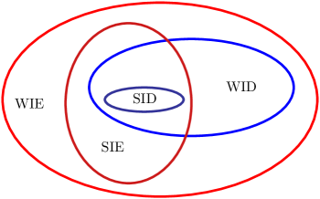
Figure 1: (Color online) Hierarchy for the sets of states WIE, SIE, WID, and SID.

To illustrate the relative character of distillability, let us consider the specific situation in which Alice (A) and Bob (B) share a bipartite mixed state of Werner type with respect to an inertial frame $\cal{S}$. Moreover, in order to complete the SR+QIT scenario, we also consider another inertial frame $\cal{S}^{\prime}$, where relatives A’ and B’ of A and B are moving with relative velocity ${\bf{v}}$ with respect to $\cal{S}$. Using the picture of Einstein’s trains, we may think that A and B are at the station platform sharing a set of mixed states, while their relatives A’ and B’ are travelling in a train sharing another couple of entangled particles of the same characteristics. The mixed state is made up of two particles, say electrons with mass $m$, having two types of degrees of freedom: momentum ${\bf{p}}$ and spin $s=\textstyle\frac{1}{2}$. The former is a continuous variable while the latter is a discrete one. By definition, we consider our logical or computational qubit to be the spin degree of freedom. Each particle is assumed to be localized, as in a box, and its momentum ${\bf{p}}$ will be described by the same Gaussian distribution. We assume that the spin degrees of freedom of particles $A$ and $B$ are decoupled from their respective momentum distributions and form the state

$$\rho^{AB}_{\cal{S}}:=F|\Psi^{-}_{{\bf{q}}}\rangle\langle\Psi^{-}_{{\bf{q}}}| \!\!\!\!\!\!+\frac{1-F}{3}\bigg{(}|\Psi^{+}_{{\bf{q}}}\rangle\langle\Psi^{+}_{{\bf{q}}}|$$ (2)

$$+|\Phi^{-}_{{\bf{q}}}\rangle\langle\Phi^{-}_{{\bf{q}}}|+|\Phi^{+}_{{\bf{q}}}\rangle\langle\Phi^{+}_{{\bf{q}}}|\bigg{)}.$$

Here, $F$ is a parameter such that $0\leq F\leq 1$,

$$\!\!\!\!\!\!\!\!|\Psi^{\pm}_{{\bf{q}}}\rangle\!\! := \!\!\frac{1}{\sqrt{2}}[\Psi_{1}^{(\rm a)}({\bf{q_{a}}})\Psi_{2}^{(\rm b)}({\bf{q_{b}}})\pm\Psi_{2}^{(\rm a)}({\bf{q_{a}}})\Psi_{1}^{(\rm b)}({\bf{q_{b}}})],$$

$$\!\!\!\!\!\!|\Phi^{\pm}_{{\bf{q}}}\rangle\!\!\! := \!\!\!\frac{1}{\sqrt{2}}[\Psi_{1}^{(\rm a)}({\bf{q_{a}}})\Psi_{1}^{(\rm b)}({\bf{q_{b}}})\pm\Psi_{2}^{(\rm a)}({\bf{q_{a}}})\Psi_{2}^{(\rm b)}({\bf{q_{b}}})],$$ (3)

where ${\bf{q_{a}}}$ and ${\bf{q_{b}}}$ are the corresponding momentum vectors of particles $A$ and $B$, as seen in $\cal{S}$, and

$$\Psi_{1}^{(\rm a)}({\bf{q_{a}}}) := {\cal G}({\bf{q_{a}}})|\!\!\uparrow\rangle=\left(\begin{array}[]{cccc}{\cal G}({\bf{q_{a}}})\\ 0\\ \end{array}\right)$$ (6)

$$\Psi_{2}^{(\rm a)}({\bf{q_{a}}}) := {\cal G}({\bf{q_{a}}})|\!\!\downarrow\rangle=\left(\begin{array}[]{cccc}0\\ {\cal G}({\bf{q_{a}}})\\ \end{array}\right)$$ (9)

$$\Psi_{1}^{(\rm b)}({\bf{q_{b}}}) := {\cal G}({\bf{q_{b}}})|\!\!\uparrow\rangle=\left(\begin{array}[]{cccc}{\cal G}({\bf{q_{b}}})\\ 0\\ \end{array}\right)$$ (12)

$$\Psi_{2}^{(\rm b)}({\bf{q_{b}}}) := {\cal G}({\bf{q_{b}}})|\!\!\downarrow\rangle=\left(\begin{array}[]{cccc}0\\ {\cal G}({\bf{q_{b}}})\\ \end{array}\right),$$ (15)

with Gaussian momentum distributions ${\cal G}({\bf{q}}):=\pi^{-3/4}w^{-3/2}\exp(-{\rm q}^{2}/2w^{2})$, being ${\rm q}:=|{\bf{q}}|$. $|\!\!\uparrow\rangle$ and $|\!\!\downarrow\rangle$ represent spin vectors pointing up and down along the $z$-axis, respectively. If we trace momentum degrees of freedom in Eq. (3), we obtain the usual spin Bell states, $\{|\Psi^{-}\rangle,|\Psi^{+}\rangle,|\Phi^{-}\rangle,|\Phi^{+}\rangle\}$. If we do the same in Eq. (2), we remain with the usual spin Werner state Werner

$$\left(\begin{array}[]{cccc}\frac{1-F}{3}&0&0&0\\ 0&\frac{2F+1}{6}&\frac{1-4F}{6}&0\\ 0&\frac{1-4F}{6}&\frac{2F+1}{6}&0\\ 0&0&0&\frac{1-F}{3}\\ \end{array}\right),$$ (20)

written in matrix form, out of which Bell state $|\Psi^{-}\rangle$ can be distilled if, and only if, $F>1/2$.

We consider also another pair of similar particles, $A^{\prime}$ and $B^{\prime}$, with the same state as $A$ and $B$, $\rho^{A^{\prime}B^{\prime}}_{\cal{S}^{\prime}}=\rho^{AB}_{\cal{S}}$, but seen in another reference frame $\cal{S}^{\prime}$. The frame $\cal{S}^{\prime}$ moves with velocity ${\bf{v}}$ along the $x$-axis with respect to the frame $\cal{S}$. When we want to describe the state of $A^{\prime}$ and $B^{\prime}$ as observed from frame $\cal{S}$, rotations on the spin variables, conditioned to the value of the momentum of each particle, have to be introduced. These conditional spin rotations, considered first by Wigner Wigner , are a natural consequence of Lorentz transformations. In general, Wigner rotations entangle spin and momentum degrees of freedom for each particle. We want to encode quantum information in the two qubits determined by the spin degrees of freedom of our two spin-$1/2$ systems. However, the reduced two-spin state, after a Lorentz transformation, increases its entropy and reduces its initial degree of entanglement. If we consider the velocities of the particles as having only non-zero components in the $z$-axis, each state vector of $A^{\prime}$ and $B^{\prime}$ in Eq. (15) transforms as

$$\Psi_{1}({\bf{q}})=\left(\begin{array}[]{cccc}{\cal G}({\bf{q}})\\ 0\\ \end{array}\right)\rightarrow\Lambda[\Psi_{1}({\bf{q}})]=\left(\begin{array}[]{cccc}\cos\theta_{{\bf{q}}}\\ \sin\theta_{{\bf{q}}}\\ \end{array}\right){\cal G}({\bf{q}})$$ (25)

$$\Psi_{2}({\bf{q}})=\left(\begin{array}[]{cccc}0\\ {\cal G}({\bf{q}})\\ \end{array}\right)\rightarrow\Lambda[\Psi_{2}({\bf{q}})]=\left(\begin{array}[]{cccc}-\sin\theta_{{\bf{q}}}\\ \,\,\,\,\,\cos\theta_{{\bf{q}}}\\ \end{array}\right){\cal G}({\bf{q}}),$$ (30)

(31)

where $\cos\theta_{{\bf{q}}}$ and $\sin\theta_{{\bf{q}}}$ express Wigner rotations conditioned to the value of the momentum vector.

The most general bipartite density matrix in the rest frame for arbitrary spin-1/2 states and Gaussian product states in momentum, is spanned by the tensor products of $\Psi^{(\rm a)}_{1}$, $\Psi^{(\rm a)}_{2}$, $\Psi^{(\rm b)}_{1}$, and $\Psi^{(\rm b)}_{2}$, and can be expressed as

$$\rho=\sum_{ijkl=1,2}C_{ijkl}\Psi^{(\rm a)}_{i}({\bf{q_{a}}})\otimes\Psi^{(\rm b)}_{j}({\bf{q_{b}}})[\Psi^{(\rm a)}_{k}({\bf{q_{a}^{\prime}}})\otimes\Psi^{(\rm b)}_{l}({\bf{q_{b}^{\prime}}})]^{{\dagger}}.$$ (32)

Under a boost, Eq. (32) will transform into

$$\Lambda\rho\Lambda^{{\dagger}}\!\!\! = \!\!\!\!\!\sum_{ijkl=1,2}C_{ijkl}\Lambda^{(\rm a)}[\Psi^{(\rm a)}_{i}({\bf{q_{a}}})]\otimes\Lambda^{(\rm b)}[\Psi^{(\rm b)}_{j}({\bf{q_{b}}})]$$ (33)

$$\times\{\Lambda^{(\rm a)}[\Psi^{(\rm a)}_{k}({\bf{q_{a}^{\prime}}})]\otimes\Lambda^{(\rm b)}[\Psi^{(\rm b)}_{l}({\bf{q_{b}^{\prime}}})]\}^{{\dagger}}.$$

Tracing out the momentum degrees of freedom, we obtain

$$\mathrm{Tr}_{\rm{\bf{q_{a}}},{\bf{q_{b}}}} (\Lambda\rho\Lambda^{{\dagger}})$$ (34)

$$= \!\!\!\!\!\!\!\!\sum_{ijkl=1,2}C_{ijkl}\mathrm{Tr}_{\rm{\bf{q_{a}}}}(\Lambda^{(\rm a)}[\Psi^{(\rm a)}_{i}({\bf{q_{a}}})]\{\Lambda^{(\rm a)}[\Psi^{(\rm a)}_{k}({\bf{q_{a}}})]\}^{{\dagger}})$$

$$\otimes\mathrm{Tr}_{\rm{\bf{q_{b}}}}(\Lambda^{(\rm b)}[\Psi^{(\rm b)}_{j}({\bf{q_{b}}})]\{\Lambda^{(\rm b)}[\Psi^{(\rm b)}_{l}({\bf{q_{b}}})]\}^{{\dagger}}).$$

Following Peres et al. SRQIT1 , we compute the Lorentz transformed density matrix of state $\Psi_{1}$, after tracing out the momentum. The expression, to first order in $w/m$, reads

$$\mathrm{Tr}_{\rm{\bf{q}}}[\Lambda\Psi_{1}(\Lambda\Psi_{1})^{{\dagger}}]=\frac{1}{2}\left(\begin{array}[]{cc}1+n_{z}^{\prime}&0\\ 0&1-n_{z}^{\prime}\end{array}\right),$$ (35)

where $n^{\prime}_{z}:=1-\left(\frac{w}{2m}\tanh\frac{\alpha}{2}\right)^{2}$ and $\cosh\alpha:=\gamma=(1-\beta^{2})^{-1/2}$. Larger values of $w/m$ are possible and mathematically correct GingrichAdami , though not necessarily physically consistent. First, the Newton-Wigner localization problem Sakurai prevents us from considering momentum distributions with $w\lesssim m$. In that case, particle creation would manifest and our model, relying on a bipartite state of the Fock space, would break down. Second, $w\sim m$ would produce fast wave-packet spreading, yielding an undesired particle delocalization.

This can be generalized to the other three tensor products involving $\Psi_{1}$ and $\Psi_{2}$,

$$\mathrm{Tr}_{\rm{\bf{q}}}[\Lambda\Psi_{2}(\Lambda\Psi_{2})^{{\dagger}}] = \frac{1}{2}\left(\begin{array}[]{cc}1-n_{z}^{\prime}&0\\ 0&1+n_{z}^{\prime}\end{array}\right),$$ (38)

$$\mathrm{Tr}_{\rm{\bf{q}}}[\Lambda\Psi_{1}(\Lambda\Psi_{2})^{{\dagger}}] = \frac{1}{2}\left(\begin{array}[]{cc}0&1+n^{\prime}_{z}\\ -(1-n_{z}^{\prime})&0\end{array}\right),$$ (41)

$$\mathrm{Tr}_{\rm{\bf{q}}}[\Lambda\Psi_{2}(\Lambda\Psi_{1})^{{\dagger}}] = \frac{1}{2}\left(\begin{array}[]{cc}0&-(1-n^{\prime}_{z})\\ 1+n_{z}^{\prime}&0\end{array}\right).$$ (44)

With the help of Eqs. (34-44), it is possible to compute the effects of the Lorentz transformation, associated with a boost in the $x$-direction, on any density matrix of two spin-1/2 particles with factorized Gaussian momentum distributions. In particular, Eq. (2) is reduced to

$$\left(\!\!\!\begin{array}[]{cccc}\frac{1}{4}+c_{F}{n^{\prime}_{z}}^{2}&0&0&c_{F}({n^{\prime}_{z}}^{2}-1)\\ 0&\frac{1}{4}-c_{F}{n^{\prime}_{z}}^{2}&c_{F}({n^{\prime}_{z}}^{2}+1)&0\\ 0&c_{F}({n^{\prime}_{z}}^{2}+1)&\frac{1}{4}-c_{F}{n^{\prime}_{z}}^{2}&0\\ c_{F}({n^{\prime}_{z}}^{2}-1)&0&0&\frac{1}{4}+c_{F}{n^{\prime}_{z}}^{2}\\ \end{array}\!\!\!\right),\\$$ (45)

where $c_{F}:=\frac{1-4F}{12}$. We can apply now the positive partial transpose (PPT) criterion Peres ; Horodeckis1 to know whether this state is entangled and distillable. Due to the box-inside-box structure of Eq. (45), it is possible to diagonalize its partial transpose in a simple way, finding the eigenvalues

$$x_{1}=\frac{2F+1}{6}\,\,,\hskip 14.22636ptx_{2}=\frac{1-F}{3}+\frac{1-4F}{6}{n^{\prime}_{z}}^{2}\,\,,$$

$$x_{3}=\frac{1-F}{3}-\frac{1-4F}{6}{n^{\prime}_{z}}^{2}\,\,,\hskip 14.22636ptx_{4}=\frac{2F+1}{6}\,\,.$$ (46)

Given that $F>0$, $x_{1}$ and $x_{4}$ are always positive, and also $x_{3}$ for $0<{n^{\prime}_{z}}<1$. The eigenvalue $x_{2}$ is negative if, and only if, $F>N^{\prime}_{z}$, where $N^{\prime}_{z}:=(2+{n^{\prime}_{z}}^{2})/(2+4{n^{\prime}_{z}}^{2})$. The latter implies that in the interval

$$\frac{1}{2}<F<N^{\prime}_{z}$$ (47)

distillability of state $|\Psi^{-}\rangle$ is possible for the spin state in A and B, but impossible for the spin state in A’ and B’, both described in frame $\cal{S}$. We plot in Fig. 2 the behavior of $N^{\prime}_{z}$ as a function of the rapidity $\alpha$. The region below the curve (ND) corresponds to the $F$ values for which distillation is not possible in the Lorentz transformed frame. On the other hand, the region above the curve (D), corresponds to states which are distillable for the corresponding values of $n^{\prime}_{z}$. Notice that there are values of $F$ for which the Werner states are weak isodistillable and weak isoentangled, corresponding to the states in the region D above the curve for the considered range of $n^{\prime}_{z}$. On the other hand, there are states that will change from distillable (entangled) into separable for a certain value of $n^{\prime}_{z}$, showing the relativity of distillability and separability.

Figure 2: $N^{\prime}_{z}$ of Eq. (47) vs. the rapidity $\alpha$, for $w/2m=0.1$.

The study of strongly isoentangled and strongly isodistillable two-spin states is a much harder task that will depend on the entanglement measure we choose. We believe that these cases impose demanding conditions and, probably, this kind of states does not exist. However we would like to give a plausibility argument to justify this conjecture. Our argument is based on two mathematical points: (i) analytic continuation is a mathematical tool that allows to extend the analytic behavior of a function to a region where it was not initially defined, and (ii) an analytic function is either constant or it changes along all its interval of definition. Point (i) will allow us to extend analytically our calculation to $n^{\prime}_{z}=0$, an unphysical but mathematically convenient limit. Point (ii) will be applied to any well-behaved entanglement measure. We consider then a general spin density matrix

$$\rho:=\left(\!\!\!\begin{array}[]{cccc}a_{1}&b_{1}&b_{2}&b_{3}\\ b_{1}^{*}&a_{2}&c_{1}&c_{2}\\ b_{2}^{*}&c_{1}^{*}&a_{3}&d\\ b_{3}^{*}&c_{2}^{*}&d^{*}&a_{4}\\ \end{array}\!\!\!\right),$$ (52)

where $a_{1}$, $a_{2}$, $a_{3}$, and $a_{4}$ are real, and $\sum_{i}a_{i}=1$. The analytic continuation of the Lorentz transformed state, according to Eqs. (34-44), in the limit $n^{\prime}_{z}\rightarrow 0$, is

$$\left(\!\!\!\begin{array}[]{cccc}1/4&\frac{i(\mathrm{\Im}b_{1}+\mathrm{\Im}d)}{2}&\frac{i(\mathrm{\Im}b_{2}+\mathrm{\Im}c_{2})}{2}&\frac{(\mathrm{\Re}b_{3}-\mathrm{\Re}c_{1})}{2}\\ \frac{-i(\mathrm{\Im}b_{1}+\mathrm{\Im}d)}{2}&1/4&\frac{(-\mathrm{\Re}b_{3}+\mathrm{\Re}c_{1})}{2}&\frac{i(\mathrm{\Im}b_{2}+\mathrm{\Im}c_{2})}{2}\\ \frac{-i(\mathrm{\Im}b_{2}+\mathrm{\Im}c_{2})}{2}&\frac{(-\mathrm{\Re}b_{3}+\mathrm{\Re}c_{1})}{2}&1/4&\frac{i(\mathrm{\Im}b_{1}+\mathrm{\Im}d)}{2}\\ \frac{(\mathrm{\Re}b_{3}-\mathrm{\Re}c_{1})}{2}&\frac{-i(\mathrm{\Im}b_{2}+\mathrm{\Im}c_{2})}{2}&\frac{-i(\mathrm{\Im}b_{1}+\mathrm{\Im}d)}{2}&1/4\\ \end{array}\!\!\!\right),$$ (57)

where $\Re$ and $\Im$ denote the real and imaginary parts. This state is separable because its eigenvalues, given by

$$\lambda_{1,2} = \frac{1}{4}[1-2\mathrm{\Re}(b_{3}-c_{1})\pm 2\mathrm{\Im}(b_{1}+b_{2}+c_{2}+d)]$$

$$\lambda_{3,4} = \frac{1}{4}[1+2\mathrm{\Re}(b_{3}-c_{1})\pm 2\mathrm{\Im}(b_{1}-b_{2}-c_{2}+d)]$$

(58)

coincide with the corresponding ones for the partial transpose matrix. In this case, $\lambda_{1}\leftrightarrow\lambda_{4}$, and $\lambda_{2}\leftrightarrow\lambda_{3}$. So, according to the PPT criterion, the analytic continuation of the Lorentz transformed density matrix of all two spin-1/2 states, with factorized Gaussian momentum distributions, converges to a separable state in the limit of $n^{\prime}_{z}\rightarrow 0$ comment . Our analytic calculation holds for $n^{\prime}_{z}\lesssim 1$, leaving out of reach the case $n^{\prime}_{z}=0$. However, any analytic measure of entanglement, due to this behavior of the analytic continuation at $n^{\prime}_{z}=0$, is forced to change with $n^{\prime}_{z}$ for $n^{\prime}_{z}\lesssim 1$, except for states separable in all frames. In this way, we give evidence of the non-existence of strong isoentangled and isodistillable states, for variations of the parameter $n^{\prime}_{z}$ under the present assumptions.

From a broader perspective, our analysis considered the invariance of entanglement and distillability of a two spin-$1/2$ system under a particular completely positive (CP) map, the one determined by the local Lorentz-Wigner transformations. The study of similar properties in the context of general CP maps is an important problem that, to our knowledge, has not received much attention in QIT, and that will require a separate and more abstract analysis. Moreover, for higher dimensional spaces, like a two spin-$1$ system (qutrits), the notion of relativity of bound entanglement will also arise Horodeckis2 .

In summary, the concepts of weak and strong isoentantangled and isodistillable states were introduced, which should help to understand the relationship between special relativity and quantum information theory. The study of Werner states allowed us to show that distillability is a relative concept, depending on the frame in which it is observed. We have proven the existence of weak isoentangled and weak isodistillable states in our range of validity of the parameter $n^{\prime}_{z}$. We also conjectured the non-existence of strong isoentangled and isodistillable two-spin states. We give evidence for this result relying on the analytic continuation of the Lorentz transformed spin density matrix for a general two spin-1/2 particle state with factorized momentum distributions.

L.L. acknowledges financial support from Spanish MEC through FPU grant AP2003-0014, CSIC 2004 5 0E 271 and FIS2005-05304 projects. M.A.M.-D. thanks DGS for grant under contract BFM 2003-05316-C02-01. E.S. acknowledges support from SFB 631, EU RESQ and EuroSQIP projects.

References

• (1) M. Nielsen and I. Chuang, Quantum Computation and Quantum Information (Cambridge University Press, Cambridge, England, 2000).
• (2) A. Galindo and M. A. Martín-Delgado, Rev. Mod. Phys. 74, 347 (2002).
• (3) C. H. Bennett, G. Brassard, S. Popescu, B. Schumacher, J. A. Smolin, and W. K. Wootters, Phys. Rev. Lett. 76, 722 (1996).
• (4) H. Bombín and M. A. Martín-Delgado, Phys. Rev. A 72, 032313 (2005).
• (5) R. F. Werner, Phys. Rev. A 40, 4277 (1989).
• (6) W. Rindler, Relativity (Oxford University Press, New York, 2001).
• (7) R. Verch and R.F. Werner, Rev. Math. Phys. 17, 545 (2005).
• (8) A. Peres and D. R. Terno, Rev. Mod. Phys. 76, 93 (2004).
• (9) A. Peres, P. F. Scudo, and D. R. Terno, Phys. Rev. Lett. 88, 230402 (2002).
• (10) E. Wigner, Annals of Mathematics, 40, 39 (1939).
• (11) S.D. Bartlett and D.R. Terno, Phys. Rev. A 71, 012302 (2005).
• (12) P. M. Alsing and G. J. Milburn, Quantum Inf. Comput. 2, 487 (2002).
• (13) J. Pachos and E. Solano, Quantum Inf. Comput. 3, 115 (2003).
• (14) R. M. Gingrich and C. Adami Phys. Rev. Lett. 89, 270402 (2002).
• (15) A. Peres, Phys. Rev. Lett. 77, 1413 (1996).
• (16) M. Horodecki, P. Horodecki, and R. Horodecki, Phys. Lett. A 223, 1 (1996).
• (17) J.J. Sakurai, Advanced Quantum Mechanics (Addison-Wesley, New York, 1967), p. 119.
• (18) We consider $n^{\prime}_{z}\rightarrow 0$ to support our conjecture, though we know from previous arguments that it is unphysical.
• (19) M. Horodecki, P. Horodecki, and R. Horodecki, Phys. Rev. Lett. 80, 5239 (1998).