Qubit Complexity of Continuous Problems

Abstract

The number of qubits used by a quantum algorithm will be a crucial computational resource for the foreseeable future. We show how to obtain the classical query complexity for continuous problems. We then establish a simple formula for a lower bound on the qubit complexity in terms of the classical query complexity.

I Introduction

There are two major motivations for studying algorithms and complexity of continuous problems.

1. Many scientific problems have continuous formulations. Examples include path integration, Feynman-Kac path integration, and the Schrödinger equation.

2. Are quantum computers more powerful than classical computers for important scientific problems? How much more powerful?

To answer these questions one must know the classical computational complexity of the problem. There are especially constructed problems such as Simon’s problem Simon (1997) for which the quantum speedup is known; see also Bennett et al. (1997). Furthermore, it is known that quantum computers enjoy quadratic speedup for search of an unordered database Grover (1997). Knowing the quantum speedup for such a discrete problem is the exception. Generally, for discrete problems we do not know the computational complexity. (Examples of discrete problems are 3-SAT and the traveling salesman problem.) We have to settle for the conjecture that the complexity hierarchy does not collapse. A famous example of this conjecture is that $\rm{P}\neq\rm{NP}$. Thus although is is widely believed that Shor’s algorithm Shor (1997) gives an exponential speedup it is only a conjecture because the classical computational complexity of integer factorization is an important open problem.

In what follows it is important to stress the difference between the cost of an algorithm for solving a given problem, and the computational complexity of this problem. The computational complexity (for brevity, the complexity) is the minimal computational resources needed to solve the problem. Examples of computational resources, which have been studied, include memory, time, and communication on a classical computer and qubits, quantum gates and queries on a quantum computer. For the foreseeable future qubits will be a limiting resource and in this paper we’ll give a general lower bound on the qubit complexity for continuous problems.

For continuous problems we often know the classical complexity. There is a large literature in the field of information-based complexity which studies problems with partial and/or contaminated information; see Traub et al. (1988); Traub and Werschulz (1998) and the references therein. Since functions of a continuous variable cannot generally be input into a digital computer, the computer has only partial information about them. As we shall see in Section II this makes it possible to use an adversary argument to get a lower bound on the classical query complexity, and, therefore, on the total complexity of many continuous problems.

Most continuous problems arising in practice cannot be solved analytically; they must be solved numerically. Since a digital computer has only partial information about the input function the problem can only be solved approximately, to within an error threshold ${\varepsilon}$. If one insists on an error at most ${\varepsilon}$ for all inputs in a class $F$ (the worst case setting) it’s been shown that for many multivariate problems the complexity is exponential in the number of variables. This is known as the curse of dimensionality and such problems are said to be intractable. Note that for continuous problems many problems are known to be intractable while for discrete problems the intractability of NP-hard problems is only conjectured; see Remark II.4.

There are two major ways to break the curse of dimensionality, see (Traub and Werschulz, 1998, p. 24). We can weaken the worst case assurance, accepting instead a stochastic assurance such as in the randomized setting. The Monte Carlo algorithm is known to be optimal for integration in this setting if $F$ is the class of bounded continuous functions. Or we can change the class $F$ of inputs. By suitable choices of $F$ we can sometimes provide a worst case guarantee while breaking intractability.

We outline the remainder of the paper. In Section II we illustrate the adversary argument which will provide us with the classical information complexity. We use a very simple example to do this. In Section III we provide a more general formulation and introduce notation. In the concluding section we’ll prove a general theorem giving a lower bound on the qubit complexity in terms of the classical query complexity.

II Classical information complexity

We will illustrate the adversary argument used to obtain the classical query complexity using a very simple example. The same idea can be applied very generally Traub et al. (1988); Traub and Werschulz (1998).

We want to compute $I(f)=\int_{0}^{1}f(x)\,dx$. Call $f$ the mathematical input. For most integrands we can’t use the fundamental theorem of calculus to compute the integral analytically; we have to approximate it numerically. Although we can input the symbolic form of $f$ into a digital computer it doesn’t help us to compute the integral. We compute

$$y_{f}=[f(t_{1}),\dots,f(t_{n})]$$

at $n$ a priori chosen deterministic points $t_{i}$, $i=1,\dots,n$. Given $y_{f}$, there are an infinite number of functions with the same $y_{f}$. That is, we have only partial information about the mathematical input. Even though the functions may have the same $y_{f}$ their integrals may be very different. Let $G$ be the set of functions with the same $y_{f}$; see Figure 1.

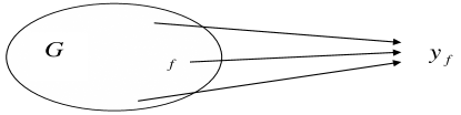
Figure 1: Indistinguishable functions

If we only assume that $f$ is, say, Riemann-integrable the classical query complexity is infinite, i.e, we cannot achieve any desired accuracy no matter how large $n$ is. To get finite complexity we have to make a promise about $f$. With the promise that the absolute value of the functions under consideration is uniformly bounded by a known constant is it is easy to show the complexity is still infinite. Thus we further restrict the class of inputs and assume that our function belongs to

$$F=\left\{f:\;|f^{\prime}(x)|\leq L,\quad x\in[0,1]\right\}.$$

Let $K=F\cap G$. The functions in $K$ are indistinguishable; see Figure 2.

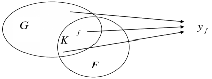
Figure 2: Restrict the class of functions

Let $H$ denote the set $I(\tilde{f})$, $\tilde{f}\in K$. It is easy to show that $H$ is an interval and that its length varies with $y_{f}$, $n$ and the points $t_{1},\dots,t_{n}$. Any number in $H$ is a potential approximation to the integral. A measure of the intrinsic uncertainty in our approximations is the size of $H$. There is a standard concept of the size of a set; it is the radius of the smallest ball containing the set. We call this radius the radius of information, $rad$, because its magnitude depends on how much information we have about the true $f$. It is easy to show that we can guarantee an ${\varepsilon}$-approximation iff $rad\leq{\varepsilon}$. Let $m({\varepsilon})$ be the minimum number of function evaluations needed to solve the problem to within ${\varepsilon}$. The condition $rad\leq{\varepsilon}$ implies that if we compute less than $m({\varepsilon})$ function evaluations there does not exist any algorithm which solves the problem with error ${\varepsilon}$. See (Traub and Werschulz, 1998, Section II.2) for a general discussion of the radius of information.

Let $\mathbf{c}$ be the cost of a query, that is of a function evaluation. We define the classical query complexity, ${\rm comp}^{\rm query}_{\rm clas}({\varepsilon})$, as

$${\rm comp}^{\rm query}_{\rm clas}({\varepsilon})=\mathbf{c}\;m({\varepsilon}).$$ (1)

The query complexity is the minimum amount that must be paid to obtain the information about $f$ needed to compute $I(f)$ to within ${\varepsilon}$.

In the concluding section we will see how the classical query complexity is used to lower bound the quantum qubit complexity. We conclude this section with some remarks.

Remark II.1.

The type of argument we have used in this section is called an adversary argument because if we don’t collect enough information an imagined adversary can claim the mathematical input is a function $g$ for which $I(g)$ is very different than $I(f)$, foiling the assurance that we’ve computed an ${\varepsilon}$-approximation to $I(f)$.

Remark II.2.

Note that there has been no mention of how $y_{f}=[f(t_{1}),\dots,f(t_{n})]$ is used to approximate the integral $I(f)$. This can be done by an algorithm $\phi$ of the form

$$\phi(f)=\sum_{j=1}^{n}a_{j}f(t_{j}).$$

There is a large literature on the optimal choice of the coefficients $a_{j}$ in $\phi$, and on the optimal choice of the points $t_{j}$; see, for example Traub and Werschulz (1998). Part of the power of the approach we’ve illustrated here is that decisions concerning information can be separated from decisions regarding algorithms.

Remark II.3.

The mathematical tools for lower and upper bounds on classical query complexity (and other types of complexity) are often deep but this example gives the idea of the adversary argument.

Remark II.4.

Why can we obtain the complexity of continuous problems whereas we have to settle for conjectures about the complexity hierarchy for discrete problems? For continuous problems we have partial information and we can use the adversary argument to get lower bounds. For discrete problems we have complete information. For example, for the traveling salesman problem we are given the locations of the cities and these coordinates can be input into a digital computer. There is no information level and no adversary argument.

III Fundamental concepts and notation for quantum computation

A quantum algorithm consists of a sequence of unitary transformations applied to an initial state. The result of the algorithm is obtained by measuring its final state. The quantum model of computation is discussed in detail in Beals et al. (1998); Bernstein and Vazirani (1997); Bennett et al. (1997); Cleve et al. (1996); Heinrich (2002); Nielsen and Chuang (2000). We summarize this model to the extent necessary for this paper.

The initial state $|\psi_{0}\rangle$ of the algorithm is a unit vector of the Hilbert space ${\cal H}_{\nu}=\mathbb{C}^{2}\otimes\cdots\otimes\mathbb{C}^{2}$, $\nu$ times, for some appropriately chosen integer $\nu$, where $\mathbb{C}^{2}$ is the two dimensional space of complex numbers. The dimension of ${\cal H}_{\nu}$ is $2^{\nu}$. The number $\nu$ denotes the number of qubits used by the quantum algorithm.

The final state $|\psi\rangle$ is also a unit vector of ${\cal H}_{\nu}$ and is obtained from the initial state $|\psi_{0}\rangle$ through a sequence of unitary $2^{\nu}\times 2^{\nu}$ matrices, i.e.,

$$|\psi\rangle\,:=\,U_{T}Q_{f}U_{T-1}Q_{f}\cdots U_{1}Q_{f}U_{0}|\psi_{0}\rangle.$$ (2)

The unitary matrix $Q_{f}$ is called a quantum query and is used to provide information to the algorithm about a function $f$. $Q_{f}$ depends on $n$ function evaluations $f(t_{1}),\dots,f(t_{n})$, $n\leq 2^{\nu}$. The $U_{0},U_{1},\dots,U_{T}$ are unitary matrices that do not depend on $f$. The integer $T$ denotes the number of quantum queries.

For algorithms solving discrete problems, such as Grover’s algorithm for the search of an unordered database Grover (1997), the input $f$ is considered to be a Boolean function. However, classical algorithms solving continuous problems using floating or fixed point arithmetic can also be written in the form of (2). Indeed, all classical bit operations can be simulated by quantum computations, see e.g., Bernstein and Vazirani (1997).

The most commonly studied quantum query is the bit query. For a Boolean function $f:\{0,\dots,2^{m}-1\}\to\{0,1\}$, the bit query is defined by

$$Q_{f}|j\rangle|k\rangle\,=\,|j\rangle|k\oplus f(j)\rangle.$$

Here $\nu=m+1$, $|j\rangle\in{\cal H}_{m}$, and $|k\rangle\in{\cal H}_{1}$ with $\oplus$ denoting the addition modulo $2$. For a real function $f$ the query is constructed by taking the most significant bits of the function $f$ evaluated at some points $t_{j}$. More precisely, as in Heinrich (2002), the bit query for $f$ has the form

$$Q_{f}|j\rangle|k\rangle\,=\,|j\rangle|k\oplus\beta(f(\tau(j)))\rangle,$$

where the number of qubits is now $\nu=m^{\prime}+m^{\prime\prime}$ and $|j\rangle\in{\cal H}_{m^{\prime}}$, $|k\rangle\in{\cal H}_{m^{\prime\prime}}$. The functions $\beta$ and $\tau$ are used to discretize the domain $\mathcal{D}$ and the range $\mathcal{R}$ of $f$, respectively. Therefore, $\beta:\mathcal{R}\to\{0,1,\dots,2^{m^{\prime\prime}}-1\}$ and $\tau:\{0,1,\dots,2^{m^{\prime}}-1\}\to\mathcal{D}$. Hence, we compute $f$ at $t_{j}=\tau(j)$ and then take the $m^{\prime\prime}$ most significant bits of $f(t_{j})$ by $\beta(f(t_{j}))$, for the details and the possible use of ancillary qubits see Heinrich (2002).

At the end of the quantum algorithm, a measurement is applied to its final state $|\psi\rangle$. The measurement produces one of $M$ outcomes, where $M\leq 2^{\nu}$. Outcome $j\in\{0,1,\dots,M-1\}$ occurs with probability $p_{f}(j)$, which depends on $j$ and the input $f$. Knowing the outcome $j$, we compute classically the final result $\phi_{f}(j)$ of the algorithm.

In principle, quantum algorithms may have many measurements applied between sequences of unitary transformations of the form presented above. However, any algorithm with many measurements can be simulated by a quantum algorithm with only one measurement at the end Bernstein and Vazirani (1997).

We are interested in continuous problems such as multivariate and path integration, multivariate approximation, ordinary and partial differential equations, and the Sturm-Liouville eigenvalue problem. For many continuous problems we know tight quantum complexity bounds Heinrich (2002, 2003, 2004a, 2004b); Kacewicz (2004); Novak (2001); Papageorgiou and Woźniakowski (2005); Traub and Woźniakowski (2002).

Let $S$ be a linear or nonlinear operator such that

$$S:\cal{F}\to\cal{G}.$$ (3)

Typically, $\cal{F}$ is a linear space of continuous real functions of several variables, and $\cal{G}$ is a normed linear space. We wish to approximate $S(f)$ to within ${\varepsilon}$ for $f\in\cal{F}$. We approximate $S(f)$ using $n$ function evaluations $f(t_{1}),\dots,f(t_{n})$ at deterministically and a priori chosen sample points. The quantum query $Q_{f}$ encodes this information, and the quantum algorithm obtains this information from $Q_{f}$.

Without loss of generality, we consider algorithms that approximate $S(f)$ with probability $p\geq\tfrac{3}{4}$. The local error of the quantum algorithm (2) that computes the approximation $\phi_{f}(j)$, for $f\in\cal{F}$ and the outcome $j\in\{0,1,\dots,M-1\}$, is defined by

$$e(\phi_{f})\,=\,\min\bigg{\{}\,{\alpha}:\quad\sum_{j:\ \|S(f)-\phi_{f}(j)\|\,\leq\,{\alpha}\,}p_{f}(j)\geq\tfrac{3}{4}\,\bigg{\}},$$ (4)

where $p_{f}(j)$ denotes the probability of obtaining outcome $j$ for the function $f$. The worst probabilistic error of a quantum algorithm $\phi$ is defined by

$$e^{{\rm quant}}(\phi)\,=\,\sup_{f\in\cal{F}}e(\phi_{f}).$$ (5)

IV Lower bound on qubit complexity

For the foreseeable future the number of qubits used by a quantum algorithm will be a crucial computational resource. We will show how to obtain a lower bound for the number of qubits needed for algorithms that approximate continuous problems such as (3). In particular, let ${\rm comp}^{\rm qubit}({\varepsilon})$ be the minimal number of qubits required by a quantum algorithm of the form (2) approximating $S(f)$ with accuracy ${\varepsilon}$ and probability at least $\tfrac{3}{4}$.

We will derive a lower bound for the qubit complexity using facts about the classical complexity of continuous problems. A similar lower bound result was announced by H. Woźniakowski at the DARPA PI meeting in Chicago in May 2004; see Woźniakowski (2005) for his proof. The proof we present here is different and constructive. In the analysis of classical algorithms one considers the classical query cost, which depends on the number of function evaluations $n$ used by the classical algorithm. It suffices to consider deterministic classical algorithms $\phi$ in the worst case, i.e., to measure the error by

$$e^{\rm wor}(\phi,n)=\sup_{f\in F}\big{\|}S(f)-\phi(f(t_{1}),\dots,f(t_{n}))\big{\|}.$$ (6)

The classical query complexity, ${\rm comp}^{\rm query}_{\rm clas}({\varepsilon})$, of the problem (3) is the minimal number of function evaluations that are necessary for accuracy ${\varepsilon}$ times the cost of a query, i.e.,

$$m({\varepsilon})=\min\left\{n:\;\exists\;\phi{\rm\ with\ }e^{\rm wor}(\phi,n)\leq{\varepsilon}\right\},\\$$

$${\rm comp}^{\rm query}_{\rm clas}({\varepsilon})=\mathbf{c}\;m({\varepsilon}).$$ (7)

The classical query and combinatorial complexities of many continuous problems are known Traub et al. (1988); Traub and Werschulz (1998). We are now ready to show how to use classical query complexity lower bounds to derive qubit complexity lower bounds.

Recall that quantum algorithms may require some classical computations to be performed, for instance, at the end after the measurement to produce the final result, or at the beginning to prepare the initial state. These classical computations may or may not include a number of function evaluations. To exclude trivial cases that reduce the qubit complexity at the expense of classical computations, we will assume that the number of function evaluations computed by the classical components of the quantum algorithm cannot exceed the number of function evaluations obtained in superposition by the query due to quantum parallelism.

Theorem IV.1.

The qubit complexity of a quantum algorithm (2) that solves the problem (3) with accuracy ${\varepsilon}$ is bounded from below as follows

$${\rm comp}^{\rm qubit}({\varepsilon})\geq\log_{2}\left[{\rm comp}^{\rm query}_{\rm clas}(3{\varepsilon})\right]-1.$$

Proof: Consider a quantum algorithm that solves the problem with accuracy ${\varepsilon}$. This algorithm uses $Q_{f}$ which, in turn, depends on a number of function evaluations of $f$ which we denote by $n({\varepsilon})$. It follows that the number of qubits of the quantum algorithm is at least $\log_{2}n({\varepsilon})$.

A quantum algorithm that approximates (3) with accuracy ${\varepsilon}$ can be simulated by a classical algorithm. The computational cost of this simulation is not important here. The important fact is that the classical algorithm also uses $n({\varepsilon})$ function evaluations and approximates $S(f)$ with worst probabilistic error (5) less than ${\varepsilon}$.

Since the algorithm achieves error ${\varepsilon}$, the final state of the quantum algorithm, and the corresponding state of its classical simulation, contain outcomes $j$ such that $\|S(f)-\phi_{f}(j)\|\leq{\varepsilon}$, where the sum of their probabilities is $\sum_{j}p_{f}(j)\geq\tfrac{3}{4}$. Moreover, the classical simulation can compute the probabilities of all the outcomes, since it has computed all the amplitudes in the final state of the quantum algorithm.

The quantities $p_{f}(j)$ and $\phi_{f}(j)$, for all possible outcomes $j$, suffice for computing deterministically an approximation of $S(f)$ with error $3{\varepsilon}$. To see this observe that the local error (4) of a quantum algorithm can be equivalently rewritten as

$$e(\phi_{f})\,=\,\min_{A:\,\mu(A)\geq\tfrac{3}{4}}\max_{j\in A}\big{\|}S(f)-\phi_{f}(j)\big{\|},$$ (8)

where $A\subset\{0,1,\dots,M-1\}$ and $\mu(A)=\sum_{j\in A}p_{f}(j)$. Consider all sets of outcomes where the sum of the respective probabilities is at least $\tfrac{3}{4}$. From these discard any set that contains outcomes $j\neq k$ such that $\|\phi_{f}(j)-\phi_{f}(k)\|>2{\varepsilon}$.

Let $A$ denote one of the remaining sets of outcomes then $\mu(A^{*})=\sum_{j\in A^{*}}p_{f}(j)\geq\tfrac{3}{4}$ and $\|\phi_{f}(j)-\phi_{f}(k)\|\leq 2{\varepsilon}$, $j,k\in A$. The fact that $e(\phi_{f})\leq{\varepsilon}$, equation (8) and the triangle inequality imply that $A$ exists.

There exists $j^{*}\in A$ such that $\|S(f)-\phi_{f}(j^{*})\|\leq{\varepsilon}$. Indeed, if we assume that $\|S(f)-\phi_{f}(j)\|>{\varepsilon}$, for all $j\in A$, then the quantum algorithm cannot have accuracy ${\varepsilon}$ with probability at least $\tfrac{3}{4}$, and we reach a contradiction.

The triangle inequality yields that $\|S(f)-\phi_{f}(j)\|\leq\|S(f)-\phi_{f}(j^{*})\|+\|\phi_{f}(j^{*})-\phi_{f}(j)\|\leq 3{\varepsilon}$, for any $j\in A$. Hence, we have obtained a deterministic classical algorithm that solves the problem with error $3{\varepsilon}$.

By our assumption, the classical components of the quantum algorithm may contain a number of function evaluations up to $n({\varepsilon})$ which implies

$$2n({\varepsilon})\geq{\rm comp}^{\rm query}_{\rm clas}(3{\varepsilon}).$$ (9)

Since the quantum algorithm must have at least $\log_{2}n({\varepsilon})$ qubits, as we indicated at the beginning of the proof, equation (9) implies that the qubit complexity of the quantum algorithm is bounded from below as follows

$${\rm comp}^{\rm qubit}({\varepsilon})\geq\log_{2}n({\varepsilon})\geq\log_{2}\left[{\rm comp}^{\rm query}_{\rm clas}(3{\varepsilon})\right]-1$$

and the proof is complete.  

As we have already indicated quantum algorithms may have several measurements. They are sequences of quantum algorithms with a single measurement, i.e., a sequences of algorithms of the form (2), and the resulting algorithm has success probability, say, $\tfrac{3}{4}$. The individual quantum algorithms may use different numbers of qubits, and we denote by $k$ the maximum of these numbers. One may reduce $k$ not only at the expense of classical function evaluations but also by considering extremely long sequences of quantum algorithms with a single measurement. Therefore, to exclude such trivial cases we will assume that the total number of classical function evaluations used by the classical components of a sequence of quantum algorithms is a polynomial in $2^{k}$, and so is the number of quantum algorithms with a single measurement that have been combined together to form the quantum algorithm with several measurements. Under these conditions we have the following corollary.

Corollary IV.1.

The qubit complexity of a quantum algorithm with several measurements is bounded as

$${\rm comp}^{\rm qubit}({\varepsilon})=\Omega\left(\log_{2}\left[{\rm comp}^{\rm query}_{\rm clas}(3{\varepsilon})\right]\right).$$

References

- Simon (1997) D. R. Simon, SIAM J. Comput. 26, 1474 (1997).
- Bennett et al. (1997) C. H. Bennett, E. Bernstein, G. Brassard, and U. Vazirani, SIAM J. Computing 26(5), 1510 (1997).
- Grover (1997) L. Grover, Phys. Rev. Lett. 79(2), 325 (1997), eprint quant-ph/9706033.
- Shor (1997) P. W. Shor, SIAM J. Comput. 26(5), 1484 (1997).
- Traub et al. (1988) J. F. Traub, G. W. Wasilkowski, and H. Woźniakowski, Information-Based Complexity (Academic Press, 1988).
- Traub and Werschulz (1998) J. F. Traub and A. G. Werschulz, Complexity and Information (Cambridge University Press, 1998).
- Beals et al. (1998) R. Beals, H. Buhrman, R. Cleve, M. Mosca, and R. de Wolf, Proceedings FOCS’98 p. 352 (1998), eprint quant-ph/9802049.
- Bernstein and Vazirani (1997) E. Bernstein and U. Vazirani, SIAM J. Computing 26(5), 1411 (1997).
- Cleve et al. (1996) R. Cleve, A. Ekert, C. Macchiavello, and M. Mosca, Phil. Trans. R. Soc. Lond. A. (1996).
- Heinrich (2002) S. Heinrich, J. Complexity 18(1), 1 (2002), eprint quant-ph/0105116.
- Nielsen and Chuang (2000) M. A. Nielsen and I. L. Chuang, Quantum Computation and Quantum Information (Cambridge University Press, 2000).
- Heinrich (2003) S. Heinrich, J. Complexity 19, 19 (2003).
- Heinrich (2004a) S. Heinrich, J. Complexity 20, 5 (2004a), eprint quant-ph/0305030.
- Heinrich (2004b) S. Heinrich, J. Complexity 20, 27 (2004b), eprint quant-ph/0305031.
- Kacewicz (2004) B. Z. Kacewicz, J. Complexity 21(5), 740 (2004).
- Novak (2001) E. Novak, J. Complexity 17, 2 (2001), eprint quant-ph/0008124.
- Papageorgiou and Woźniakowski (2005) A. Papageorgiou and H. Woźniakowski, Quantum Information Processing 4(2), 87 (2005), eprint quant-ph/0502054.
- Traub and Woźniakowski (2002) J. F. Traub and H. Woźniakowski, Quantum Information Processing 1(5), 365 (2002), eprint quant-ph/0109113.
- Woźniakowski (2005) H. Woźniakowski, The quantum setting with randomized queries for continuous problems (2005), in progress.