Factorizing the time evolution operator

Abstract

There is a widespread belief in the quantum physical community, and in textbooks used to teach Quantum Mechanics, that it is a difficult task to apply the time evolution operator $e^{it\hat{H}/\hbar}$ on an initial wave function. That is to say, because the hamiltonian operator generally is the sum of two operators, then it is a difficult task to apply the time evolution operator on an initial wave function $\psi(x,0)$, for it implies to apply terms like $(\hat{a}+\hat{b})^{n}$. A possible solution of this problem is to factorize the time evolution operator and then apply successively the individual exponential operator on the initial wave function. However, the exponential operator does not directly factorize, i. e. $e^{\hat{a}+\hat{b}}\neq e^{\hat{a}}e^{\hat{b}}$. In this work we present a useful procedure for factorizing the time evolution operator when the argument of the exponential is a sum of two operators, which obey specific commutation relations. Then, we apply the exponential operator as an evolution operator for the case of elementary unidimensional potentials, like the particle subject to a constant force and the harmonic oscillator. Also, we argue about an apparent paradox concerning the time evolution operator and non-spreading wave packets addressed previously in the literature.

I Introduction

Quantum Mechanics is a successful theory. Although highly counterintuitive, using it we are able to explain the microscopic world. Also, Quantum Mechanics have discovered many natural process which have culminated in practical technological applications, like the transistor and the Quantum Cryptography. However, Quantum Mechanics is a difficult field of study. For it takes many years to develop the necessary skills to understand their relevant concepts.

One of the hardest skills to develop is to understand the technique to solve the fundamental equation of Quantum Mechanics, i. e. the Schrödinger equation. In fact, there are few cases where this equation was analytically solved. One of the principal factors that impede the straightforward solution is that this equation involves not usual mathematical concepts, like operators:

$$i\hbar\frac{\partial}{\partial t}\Psi(t)=\hat{H}\Psi(t),$$ (1)

where the Hamiltonian $\hat{H}$ is an operator that has to be self-adjoint, and it is generally the sum of two or more operators, let us say:

$$\hat{H}=\hat{a}+\hat{b}.$$ (2)

In the literature, the most used technique to solve Equation (1) is to find the eigenvalues and eigenfunctions of the time independent Schrödinger equation:

$$\hat{H}\psi_{n}(x)=E_{n}\psi_{n}(x),$$ (3)

where $E_{n}$ and $\psi_{n}(x)$ are, respectively, the eigenvalues and eigenfunctions of the hamiltonian $\hat{H}$ book1 ; book2 ; book3 ; book4 . Then, the time dependent wave function is constructed taking the superposition of the eigenfunctions of the hamiltonian:

$$\Psi(x,t)=\sum_{n=0}^{\infty}e^{-iE_{n}t/\hbar}c_{n}\psi_{n}(x),$$ (4)

where $c_{n}=\int\Psi(x,0)\psi_{n}dx$ is the scalar product between the initial state of the system and the eigenfuctions of the hamiltonian. In this paper, we call this method the eigenstates method.

A second way for solving Eq. (1), if we consider a time independent Hamiltonian, is to integrate Eq. (1) with respect to time, to obtain book1 :

$$\Psi(x,t)=e^{-\frac{it}{\hbar}\hat{H}}\Psi(x,0)=e^{\hat{A}+\hat{B}}\Psi(x,0),$$ (5)

where $\Psi(x,0)$ is the initial wave vector, $\hat{A}=-(it/\hbar)\hat{a}$ and $\hat{B}=-(it/\hbar)\hat{b}$. In this paper, we call this method the evolution operator method.

Essentially, both ways for solving the Schrödinger equation are the same. This can be proved by expanding $\Psi(x,0)$ in terms of the eigenfunctions of the Hamiltonian, i.e. $\Psi(x,0)=\sum c_{n}\psi_{n}(x)$, and inserting it on the right hand side of Eq. (5) to produce Equation (4). An alternative way to solve the Schrödinger equation is the technique developed by Feynman, called the Feynman propagator method holstein2 ; gori ; barone .

The trouble with Equation (5) is that, in general, $\hat{A}$ and $\hat{B}$ do not commute. This makes difficult to apply the time evolution operator to the initial state vector given in Eq. (5). In fact, the problem is how to make the expansion of a function of noncommuting operators like that in Eq. (5), i. e. $e^{\hat{A}+\hat{B}}=\sum_{n=0}^{\infty}(1/n!)(\hat{A}+\hat{B})^{n}$, in such a way that all the $\hat{B}$ precede the $\hat{A}$, or viceversa. This problem has been already studied by many authors, and some theorems have been proved to handle this expansion. For example, Kumar proved the following expansion for a function of noncommuting operators kumar :

$$f(\hat{A}+\hat{B})=\sum_{n=0}^{\infty}\frac{1}{n!}C^{n}(\hat{A},\hat{B})f^{(n)}(\hat{A}),$$ (6)

where $C^{n}(\hat{A},\hat{B})$ is a coefficient operator given in terms of $\hat{B}$ and the commutator $[\hat{A},\hat{B}]$ kumar .

Also, Cohen has proved the following expansion theorem for the operators $\hat{x}$ and $\hat{p}$ cohen : Given a function $F(\hat{x},\hat{p})$ then

$$F^{n}(\hat{x},\hat{p})=\sum_{n=0}^{\infty}\alpha_{k}^{n}u_{k}(\hat{x})\int_{-\infty}^{\infty}u_{k}^{*}(\hat{x}+\theta)e^{(i/\hbar)\theta p}d\theta,$$ (7)

where $\alpha_{k}$ and $u_{k}(\hat{x})$ are the eigenvalue and eigenfunction of the eigenvalue problem $F(\hat{x},\hat{p})u_{k}(\hat{x})=\alpha_{k}u_{k}(\hat{x})$. In particular, the expansion for the function $(\lambda\hat{x}+\hat{p})^{n}$ has given as cohen :

$$(\lambda\hat{x}+\hat{p})^{n}=\sum_{k=0}^{[\frac{1}{2}n]}\sum_{s=0}^{n-2k}\frac{(-1)^{k}n!}{k!(n-2k)!}\left(\begin{array}[]{cc}n-2k\\ s\end{array}\right)(i\hbar/2)^{k}\lambda^{n-k-s}\hat{x}^{n-2k-s}\hat{p}^{s}.$$ (8)

In general, these expansion theorems have produced a high cumbersome expressions that are very difficult to apply.

One of the possible paths to avoid the expansion of functions of two noncommuting operators, in the case of the exponential operators, is to factorize the argument of the exponential. This approach facilitates the application of the exponential operator because now, when the exponential operator is factorized, we have only to expand the exponential of a single operator, i. e. $e^{\hat{A}}e^{\hat{B}}$, which is more simple. However, the factorization of exponential operators is not an easy task. To our best knowledge, the evolution operator method has been applied to unidimensional problems in only four other related articles blinder ; robinett ; bala ; cheng .

The main goal of this paper is twofold, first we shall show a procedure to factorize the exponential operator and, secondly, we shall show how to apply the factorized exponential operator on an initial wave function. The method of factorization that we shall present in this paper has been used in Quantum Optics. Also, this method has been proposed as a possible tool to improve some misconceptions in the teaching of Quantum Mechanics paulo . Therefore, an important objective of this paper is to review this method in order that it becomes available for the people outside these fields.

Although the three methods for solving the Schrödinger equation mentioned above have to give the same result, the evolution operator method is, in some way, quite different of the eigenstates method and the Feynman propagator. For example, in the eigenstates method we need to look for the eigenfunctions of the hamiltonian where the particle is placed; on the contrary, the evolution operator method does not give any information about the eigenfunctions of the hamiltonian. Also, the Feynman propagator method need to look for all the possible paths the particle can take from an initial wave function to a final one, and the evolution operator method does not inquire for these possible paths. In some sense, the evolution operator method is more direct than the other two.

In summary, this paper address the problem of how to factorize the exponential of a sum of operators, in order to be able to apply it as an evolution operator, when the operators obey certain commutation rules. To make the factorization we use the tool of the differential equation method wilcox ; louisell , which requires that both sides of an equation satisfy the same first-order differential equation and the same initial condition. For a review of these tools see the work of Wilcox wilcox and Lutzky lutzky . This method has been used successfully in the field of Quantum Optics yo ; yo2 ; lu1 . We shall show that this method is useful and easy to apply in the unidimensional problems of Quantum Mechanics.

This paper is organized as follows: In Section II we will present the method and show how to apply it for factorizing an exponential operator. In Section III we give a specific example when the operators obey certain commutation rules. In Subsection A of this section, we apply the found factorization to the case when the particle is subjected to a constant force. In Section IV we present the factorization of the exponential operator when its argument obeys a more complex commutation rules; in subsection A of this section the factorization found is applied to the harmonic oscillator. In subsection B of section IV, we derive another way to factorize the harmonic oscillator and we show that both factorizations give the same evolution function (In Appendix A we derive yet another way to factorize the harmonic oscillator). In Section V we address a supposed limitation of the evolution operator method, we demonstrate that the limitation is because the initial wave function used to show the apparent paradox is outside of the domain of the hamiltonian operator.

II The method

As the global purpose of this paper is pedagogical, in this section we show how the method works. Our intention is that this method can be used for researchers of any field to find the evolution state from an initial wave function. In order to be explicit we separate the method in three steps and apply it to obtain the well know Baker-Cambell-Hausdorff formula:

$$e^{(\hat{A}+\hat{B})}=e^{\hat{A}}e^{\hat{B}}e^{f([\hat{A},\hat{B}])}.\qquad\quad$$ (9)

$$\quad When\quad[\hat{A},[\hat{A},\hat{B}]]=[\hat{B},[\hat{A},\hat{B}]]=0\quad i.e.\quad[\hat{A},\hat{B}]=\delta.$$

where $\delta$ is a constant. Notice that after we have solved this easy problem we will progressively increase the difficulty of the commutation relation.

To make the factorization of the exponential of the sum of two operators we proceed as follows:

1. Firstly, we define an auxiliary function in terms of the exponential of the sum of two operators, its commutator and an auxiliary parameter $\xi$:

   $$F(\xi)=e^{\xi(\hat{A}+\hat{B})},$$ (10)

   $$F(\xi)=e^{f_{1}(\xi)[\hat{A},\hat{B}]}e^{f_{2}({\xi})\hat{A}}e^{f_{3}({\xi})\hat{B}}.$$ (11)

   Note that in Equations (10) and (11) we are defining separately $F(\xi)$ as a function and its factorization. That is to say, if $e^{f_{1}(\xi)[\hat{A},\hat{B}]}e^{f_{2}({\xi})\hat{A}}e^{f_{3}({\xi})\hat{B}}$ is the factorization of $e^{\xi(\hat{A}+\hat{B})}$, then $F(\xi)=e^{\xi(\hat{A}+\hat{B})}=e^{f_{1}(\xi)[\hat{A},\hat{B}]}e^{f_{2}({\xi})\hat{A}}e^{f_{3}({\xi})\hat{B}}$.

2. Secondly, we differentiate Equations (10) and (11) with respect to the parameter $\xi$ to obtain:

   $$\frac{dF(\xi)}{d\xi}=(\hat{A}+\hat{B})e^{\xi(\hat{A}+\hat{B})}=(\hat{A}+\hat{B})F(\xi),$$ (12)

   $$\frac{dF(\xi)}{d\xi}=\frac{df_{1}(\xi)}{d\xi}[\hat{A},\hat{B}]e^{f_{1}(\xi)[\hat{A},\hat{B}]}e^{f_{2}({\xi})\hat{A}}e^{f_{3}({\xi})\hat{B}}+$$

   $$e^{f_{1}(\xi)[\hat{A},\hat{B}]}\frac{df_{2}({\xi})}{d\xi}\hat{A}e^{f_{2}({\xi})\hat{A}}e^{f_{3}({\xi})\hat{B}}+e^{f_{1}(\xi)[\hat{A},\hat{B}]}e^{f_{2}({\xi})\hat{A}}\frac{df_{3}({\xi})}{d\xi}\hat{B}e^{f_{3}({\xi})\hat{B}}.$$ (13)

   After that, we need to put in order the operators of Equation (13). In order to make the new arrange we use the fact that the operators are self-adjoints, i. e. $e^{\xi\hat{A}}\hat{B}=\left(e^{\xi\hat{A}}\hat{B}e^{-\xi\hat{A}}\right)e^{\xi\hat{A}}$, and the well know relation: $e^{\gamma\hat{A}}\hat{B}e^{-\gamma\hat{A}}=\hat{B}+\gamma[\hat{A},\hat{B}]+\frac{\gamma^{2}}{2!}[\hat{A},[\hat{A},\hat{B}]]+\dots$, see reference louisell . That is, we have to pass the exponentials to the right in the right hand side of Equation (13). In this case:

   $$e^{f_{1}(\xi)[\hat{A},\hat{B}]}\hat{A}e^{-f_{1}(\xi)[\hat{A},\hat{B}]}=\hat{A}$$ (14)

   and

   $$e^{f_{2}(\xi)\hat{A}}\hat{B}e^{-f_{2}(\xi)\hat{A}}=\hat{B}+\delta f_{2}(\xi),$$ (15)

   where we have used the fact that $[\hat{A},\hat{B}]=\delta$. If we substitute these relations in Eq. (13) we obtain:

   $$\frac{dF(\xi)}{d\xi}=\frac{df_{1}(\xi)}{d\xi}[\hat{A},\hat{B}]e^{f_{1}(\xi)[\hat{A},\hat{B}]}e^{f_{2}({\xi})\hat{A}}e^{f_{3}({\xi})\hat{B}}+$$

   $$\frac{df_{2}({\xi})}{d\xi}\hat{A}e^{f_{1}(\xi)[\hat{A},\hat{B}]}e^{f_{2}({\xi})\hat{A}}e^{f_{3}({\xi})\hat{B}}+$$

   $$\frac{df_{3}({\xi})}{d\xi}e^{f_{1}(\xi)[\hat{A},\hat{B}]}[\hat{B}+\delta f_{2}(\xi)]e^{f_{2}({\xi})\hat{A}}e^{f_{3}({\xi})\hat{B}}.$$ (16)

   Now, using the relation $e^{f_{1}(\xi)[\hat{A},\hat{B}]}\hat{B}e^{-f_{1}(\xi)[\hat{A},\hat{B}]}=\hat{B}$ in Eq. (16) we obtain:

   $$\frac{dF(\xi)}{d\xi}=\frac{df_{1}(\xi)}{d\xi}[\hat{A},\hat{B}]e^{f_{1}(\xi)[\hat{A},\hat{B}]}e^{f_{2}({\xi})\hat{A}}e^{f_{3}({\xi})\hat{B}}+$$

   $$\frac{df_{2}({\xi})}{d\xi}\hat{A}e^{f_{1}(\xi)[\hat{A},\hat{B}]}e^{f_{2}({\xi})\hat{A}}e^{f_{3}({\xi})\hat{B}}+$$

   $$\frac{df_{3}({\xi})}{d\xi}[\hat{B}+\delta f_{2}(\xi)]e^{f_{1}(\xi)[\hat{A},\hat{B}]}e^{f_{2}({\xi})\hat{A}}e^{f_{3}({\xi})\hat{B}}.$$ (17)

   That is, we successfully passed all the exponential to the right and we can write Eq. (17) as:

   $$\frac{dF(\xi)}{d\xi}=\left\{\frac{df_{1}(\xi)}{d\xi}[\hat{A},\hat{B}]+\frac{df_{2}({\xi})}{d\xi}\hat{A}+\frac{df_{3}({\xi})}{d\xi}[\hat{B}+\delta f_{2}(\xi)]\right\}$$

   $$\times e^{f_{1}(\xi)[\hat{A},\hat{B}]}e^{f_{2}({\xi})\hat{A}}e^{f_{3}({\xi})\hat{B}}.$$ (18)

   That is, by Equation (11) we arrive to the following result:

   $$\frac{dF(\xi)}{d\xi}=\left\{\frac{df_{1}(\xi)}{d\xi}[\hat{A},\hat{B}]+\frac{df_{2}({\xi})}{d\xi}\hat{A}+\frac{df_{3}({\xi})}{d\xi}[\hat{B}+\delta f_{2}(\xi)]\right\}F(\xi).$$ (19)

3. Finally, as a third step, we must to compare the coefficients of Eq. (12) and Eq. (19), from which a set of differential equations is obtained:

   $$\frac{df_{2}(\xi)}{d\xi} = 1,$$

   $$\frac{df_{3}(\xi)}{d\xi} = 1,$$

   $$\delta\frac{df_{1}(\xi)}{d\xi}+\delta\frac{df_{3}(\xi)}{d\xi}f_{2}(\xi) = 0,$$ (20)

   subjected to the initial condition $f_{1}(0)=f_{2}(0)=f_{3}(0)=0$. In this case the solutions are:

   $$f_{2}(\xi) = \xi,$$

   $$f_{3}(\xi) = \xi,$$

   $$f_{1}(\xi) = -\frac{1}{2}\xi^{2}.$$ (21)

   After substituting Eq. (21) in Eq. (11) we arrive to the following Equation:

   $$e^{\xi(\hat{A}+\hat{B})}=e^{-\xi^{2}[\hat{A},\hat{B}]/2}e^{\xi\hat{A}}e^{\xi\hat{B}}.$$ (22)

   Setting $\xi=1$ we obtain the usual Baker-Campbell-Hausdorff formula.

This method facilitates the application of the exponential operator, because now we have to handle only individual operators function. The proposed factorization of Equation (11) is one of the possibilities, also we can define $F(\xi)$ as:

$$F(\xi)=e^{g_{1}({\xi})\hat{B}}e^{g_{2}({\xi})\hat{A}}e^{g_{3}(\xi)\hat{B}},$$ (23)

or make another arrange of the exponentials, as for example $e^{h_{1}({\xi})\hat{A}}e^{h_{2}({\xi})\hat{B}}e^{h_{3}(\xi)\hat{A}}$. Notice that Equation (23), in contrast to Equation (11), does not use the commutator in the exponential functions. This arrangement could be used to treat specific problems, as the harmonic oscillator.

In fact, when the method is dominated this arrangement is a set of crafted directions, which gives a factorization of the evolution operator. In the majority of cases, a different arrange will produce a different set of differential equations and, obviously, a different set of solutions. We give an explicit example of this fact in the case of the harmonic oscillator, see Equations (56), (48) and (63). It is very important not to confuse the Baker-Campbell-Hausdorff formula with the method addressed here. Each one represents a different way to factorize exponential operators.

On the other hand, this method can be used to improve some misconceptions of Quantum Mechanics paulo ; singh2 . Immediately we present the different cases that appear when the operators obey different commutation rules.

III Case 1: $[\hat{A},\hat{B}]=\hat{C},\quad[\hat{A},\hat{C}]=0$ and $[\hat{C},\hat{B}]=-k$

This section is organize as follows: Firstly, we make the factorization of the exponential operator when the operators obey the commutation relations given by Equation (24). Secondly, in Subsection A we use the factorized exponential to solve the problem of a particle subjected to a constant force.

Therefore, we begin the factorization of exponential operators by analyzing the case when

$$[\hat{A},\hat{B}]=\hat{C},\quad[\hat{A},\hat{C}]=0,\quad and\quad[\hat{C},\hat{B}]=-k,$$ (24)

where $\hat{A}$, $\hat{B}$ and $\hat{C}$ are operators and $k$ is a c-number (in general, we use the simbol $\hat{}$ to denote operators).

In the present case, we propose the factorization function as:

$$F(\xi)=e^{\xi(\hat{A}+\hat{B})}=e^{f(\xi)\hat{A}}e^{g(\xi)\hat{B}}e^{h(\xi)\hat{C}}e^{r(\xi)},$$ (25)

by differentiating Eq. (25) with respect to $\xi$ we obtain for the left hand side

$$\frac{dF(\xi)}{d\xi}=(\hat{A}+\hat{B})F(\xi),$$ (26)

and, for the right hand side

$$\frac{dF(\xi)}{d\xi}=\left[\frac{df}{d\xi}\hat{A}+\frac{dg}{d\xi}\hat{B}+\frac{dg}{d\xi}f(\xi)\hat{C}+\frac{dh}{d\xi}(\hat{C}+kg)+\frac{dr}{d\xi}\right]F(\xi),$$ (27)

where we have applied the fact that

$$e^{\xi\hat{A}}\hat{B}e^{-\xi\hat{A}}=\hat{B}+\xi[\hat{A},\hat{B}]+\frac{\xi^{2}}{2!}[\hat{A},[\hat{A},\hat{B}]]+\ldots,$$ (28)

and we have used the commutation relation of Eq. (24).

By equating the coefficients of Eq. (26) and Eq. (27) we obtain the following system of differential equations:

$$\frac{df(\xi)}{d\xi} = 1,$$

$$\frac{dg(\xi)}{d\xi} = 1,$$

$$\frac{dg(\xi)}{d\xi}f(\xi)+\frac{dh(\xi)}{d\xi} = 0,$$

$$kg(\xi)\frac{dh(\xi)}{d\xi}+\frac{dr(\xi)}{d\xi} = 0$$ (29)

subjected to the initial condition $F(0)=0$, which implies:

$$f(0)=g(0)=h(0)=r(0)=0.$$ (30)

By solving Eq. (29) with the initial condition stated in Eq. (30), we finally obtain

$$e^{\xi(\hat{A}+\hat{B})}=e^{(\xi^{3}/3)k}e^{\xi\hat{A}}e^{\xi\hat{B}}e^{-(\xi^{2}/2)\hat{C}}.$$ (31)

Setting $\xi=1$ we obtain the factorization we were looking for.

III.1 Application: A particle subject to a constant force

One application of the evolution operator method is when we study the time dependence of a quantum state. There have been some results in this approach when the operator is the energy of a free particle blinder , or the energy of a particle subjected to a constant force, that is $V(x)=-Fx$ robinett . In this subsection, we use the factorization found above to solve the problem of a particle subject to a constant force, whit the help of the Blinder’s method blinder . The Blinder’s method show how to apply the evolution operator like and infinite sum for a free particle:

$$e^{\frac{-it\hat{p}^{2}}{2m\hbar}}=\sum_{n=0}^{\infty}\left(\frac{i\hbar t}{2m}\right)^{n}\frac{1}{n!}\left(\frac{\partial^{2}}{\partial x^{2}}\right)^{n}.$$ (32)

For a free particle the wave function at time $t$ is obtained by operating with the evolution operator on the initial wave function. Taking as an initial wave function:

$$\Psi(x,0)=\frac{1}{(\sigma\sqrt{\pi})^{1/2}}e^{-\frac{x^{2}}{4\sigma^{2}}},$$ (33)

where $\sigma$ is the width of the wave packet. The Blinder’s method consist in the application of the identity blinder : $\frac{\partial^{2}}{\partial x^{2}}\left\{z^{-1/2}\exp\{-x^{2}/4z\}\right\}=\frac{\partial}{\partial z}\left\{z^{-1/2}\exp\{-x^{2}/4z\}\right\}$. This identity allows us to apply the evolution operator on initial wave functions like gaussian wave packets, for details see reference blinder .

For a particle subject to a constant force, i.e. $V(x)=-Fx$, the wave function at time $t$ is given by:

$$\Psi(x,t)=\exp\left[-\frac{it}{\hbar}\left(\frac{\hat{p}^{2}}{2m}-Fx\right)\right]\Psi(x,0),$$ (34)

defining $\hat{A}=\hat{p}^{2}(2m)^{-1}$, $\hat{B}=-F\hat{x}$, and using the commutation relations between $\hat{p}$ and $\hat{x}$ we can deduce the following commutation rules:

$$[\hat{A},\hat{B}]=\frac{i\hbar F}{m}\hat{p},\qquad[\hat{A},\hat{C}]=0,\qquad and\qquad[\hat{C},\hat{B}]=-\frac{\hbar^{2}F^{2}}{m},$$ (35)

where $\hat{C}=i\hbar F\hat{p}/m$. If we identify $k=\hbar^{2}F^{2}/m$, then the commutation relations of Eq. (35) are similar to that of Eq. (24). Therefore, if we use Eq. (31), we can write Eq. (34) as:

$$\Psi(x,t)=\exp\left[\frac{it^{3}F^{2}}{3\hbar m}\right]\exp\left[-\frac{it}{2m\hbar}\hat{p}^{2}\right]\exp\left[\frac{itF}{\hbar}\hat{x}\right]\exp\left[\frac{it^{2}F}{2m\hbar}\hat{p}\right]\Psi(x,0).$$ (36)

Using the theorem $\exp[\xi\hat{A}]F(\hat{B})\exp[-\xi\hat{A}]=F(\exp[\xi\hat{A}]\hat{B}\exp[-\xi\hat{A}])$ louisell , we can rearrange Eq. (36) as follows:

$$\Psi(x,t)=\exp\left[-\frac{iF^{2}t^{3}}{6m\hbar}\right]\exp\left[\frac{itF}{\hbar}\hat{x}\right]\exp\left[-\frac{it}{2m\hbar}\hat{p}^{2}\right]\exp\left[-\frac{it^{2}F}{2m\hbar}\hat{p}\right]\Psi(x,0).$$ (37)

Taking as an initial state that of Eq. (33) we finally obtain:

$$\Psi(x,t)=\left(\sigma\sqrt{2\pi}\right)^{-1/2}\left(1+(i\hbar t/2m\sigma^{2})\right)^{-1}\exp\left[\frac{iFt}{\hbar}\left(x-(Ft^{2}/6m)\right)\right]$$

$$\times\exp\left[-\frac{(x-\left(Ft^{2}/2m)\right)^{2}}{4\left(\sigma^{2}+(i\hbar t/2m)\right)}\right].$$ (38)

Equations (37) and (38) are exactly the same equations obtained by Robinett robinett .

IV Case 2: $[\hat{A},\hat{B}]=\hat{C},\quad[\hat{A},\hat{C}]=2\gamma\hat{A}$ and $[\hat{B},\hat{C}]=-2\gamma\hat{B}$

In this section, we carry out the factorization of the exponential operator when the commutation rules are given by Equation (39). Then, we will show in Subsection A that these commutation relations are the same of the harmonic oscillator. On the other hand, in Subsection B we show an alternative way of factorization for this problem, and show that the evolution given by the evolution operator are the same in both cases.

$$[\hat{A},\hat{B}]=\hat{C},\quad[\hat{A},\hat{C}]=2\gamma\hat{A}\quad[\hat{B},\hat{C}]=-2\gamma\hat{B}.$$ (39)

In this case, using an arrangement similar to Equation (23), we define the function as:

$$F(\xi)=e^{\xi(\hat{A}+\hat{B})}=e^{f(\xi)\hat{B}}e^{g(\xi)\hat{A}}e^{h(\xi)\hat{B}}.$$ (40)

By differentiating Equation (40) with respect to $\xi$, we obtain:

$$\frac{dF(\xi)}{d\xi}=(\hat{A}+\hat{B})F(\xi),$$ (41)

and

$$\frac{dF(\xi)}{d\xi}=\Bigg{\{}\left[g(\xi)\frac{dh(\xi)}{d\xi}-f(\xi)\frac{dg(\xi)}{d\xi}-\gamma g^{2}(\xi)f(\xi)\frac{dh(\xi)}{d\xi}\right]\hat{C}$$

$$\left[\frac{df(\xi)}{d\xi}+\gamma f^{2}(\xi)\frac{dg(\xi)}{d\xi}+\frac{dh(\xi)}{d\xi}-2\gamma f(\xi)g(\xi)\frac{dh(\xi)}{d\xi}+\gamma^{2}f^{2}(\xi)g^{2}(\xi)\frac{dh(\xi)}{d\xi}\right]\hat{B}$$

$$+\left[\frac{dg(\xi)}{d\xi}+\gamma g^{2}(\xi)\frac{dh(\xi)}{d\xi}\right]\hat{A}\Bigg{\}}F(\xi),$$ (42)

where we have applied the relation $e^{\xi\hat{A}}\hat{B}e^{-\xi\hat{A}}=\hat{B}+\xi[\hat{A},\hat{B}]+\frac{\xi^{2}}{2!}[\hat{A},[\hat{A},\hat{B}]]+\ldots.$

By equating Equations (41) and (42), we obtain the following system of differential equations:

$$\frac{dg(\xi)}{d\xi}+\gamma g^{2}(\xi)\frac{dh(\xi)}{d\xi}=1,$$

$$\frac{df(\xi)}{d\xi}+\gamma f^{2}(\xi)\frac{dg(\xi)}{d\xi}+\frac{dh(\xi)}{d\xi}-2\gamma f(\xi)g(\xi)\frac{dh(\xi)}{d\xi}+\gamma^{2}f^{2}(\xi)g^{2}(\xi)\frac{dh(\xi)}{d\xi}=1,$$

$$g(\xi)\frac{dh(\xi)}{d\xi}-f(\xi)\frac{dg(\xi)}{d\xi}-\gamma g^{2}(\xi)f(\xi)\frac{dh(\xi)}{d\xi}=0,$$ (43)

subjected to the initial condition $F(0)=1$, which means: $g(0)=f(0)=h(0)=0.$ By solving Equation (43), with the initial conditions, we obtain the following solutions:

$$f\left(\xi\right) = h\left(\xi\right)=\frac{1}{\sqrt{\gamma}}\tan\left(\xi\sqrt{\gamma}/2\right),$$ (44)

$$g\left(\xi\right) = \frac{1}{\sqrt{\gamma}}\sin\left(\xi\sqrt{\gamma}\right).$$ (45)

Setting $\xi=1$ we obtain the factorization we were looking for, that is Eq. (40).

As it was stated at the end of Section $2$, the factorization given in Equation (40) is only one of many possibilities. Since the operators do not commute, various orderings on the right hand side of Equation (40) represent different substituting schemes as we will show in the following subsections and in the appendix. For example, we can propose a different arrangement $F(\xi)=e^{f_{1}(\xi)\hat{A}}e^{f_{2}(\xi)\hat{B}}e^{f_{3}(\xi)\hat{A}}$, or inclusive add the commutator $\hat{C}$: $F(\xi)=e^{h(\xi)\hat{C}}e^{f(\xi)\hat{A}}e^{g(\xi)\hat{B}}$.

IV.1 Application: The one-dimensional harmonic oscillator.

One of the most important systems in Quantum Mechanics is the harmonic oscillator. For it serves both to model many physical systems occurring in nature and to show the analytical solution of the Schrödinger equation. The Schrödinger equation for this system has been solved in two ways, firstly by analytically solving the eigenvalue equation and, secondly, by defining the creation and annihilation operators book1 ; book2 . We solve here the problem using the evolution operator method. This method allows us to find the evolution for the harmonic oscillator and avoids to deal with the stationary states.

For the one-dimensional harmonic oscillator the wave function at time $t$ is given by:

$$\Psi(x,t)=\exp\left[-\frac{it}{\hbar}\left(\frac{\hat{p}^{2}}{2m}+\frac{1}{2}mw^{2}\hat{x}^{2}\right)\right]\Psi(x,0).$$ (46)

Defining $\hat{A}=-\left(itmw^{2}/2\hbar\right)\hat{x}^{2}$, $\hat{B}=-\left(it/2m\hbar\right)\hat{p}^{2}$, and using the commutation rules between $\hat{x}$ y $\hat{p}$ we can deduce the following commutation rules:

$$\left[\hat{A},\hat{B}\right]=\hat{C},\quad\left[\hat{A},\hat{C}\right]=-2w^{2}t^{2}\hat{A}\quad and\quad\left[\hat{B},\hat{C}\right]=2w^{2}t^{2}\hat{B},$$ (47)

where $\hat{C}=\frac{iw^{2}t^{2}}{2\hbar}\left(\hat{x}\hat{p}+\hat{p}\hat{x}\right)$. If we identify $\gamma=w^{2}t^{2}$, then these commutation relations correspond to that of Equation (39). Therefore, using the factorization found in Eq. (40), the Equation (46) becomes:

$$\Psi(x,t)=e^{\mu(t)\frac{d^{2}}{dx^{2}}}e^{-\delta(t)x^{2}}e^{\mu(t)\frac{d^{2}}{dx^{2}}}\Psi(x,0),$$ (48)

where

$$\mu(t) = \frac{i\hbar}{2m\omega}\tan(\omega t/2),$$

$$\delta(t) = \frac{im\omega}{2\hbar}\sin(\omega t).$$ (49)

For the one-dimensional harmonic oscillator the wave function at time $t$ is obtained by operating with the evolution operator, i. e. Eq. (48), on the initial wave function. Taking as an initial wave function:

$$\Psi(x,0)=\frac{1}{(\sigma\sqrt{\pi})^{1/2}}e^{-\frac{x^{2}}{4\sigma^{2}}},$$

we finally obtain the state of the system at any time $t$ is:

$$\Psi(x,t)=\frac{1}{(\sigma\sqrt{\pi})^{1/2}}\frac{1}{\sqrt{\cos(\omega t)+(2i\hbar/m\omega)(1/4\sigma^{2})\sin(\omega t)}}$$

$$\times\exp\left[-\frac{(im\omega/2\hbar)\sin(\omega t)-(1/2\sigma^{2})\sin^{2}(\omega t/2)+(1/4\sigma^{2})}{\cos(\omega t)+(2i\hbar/m\omega)(1/4\sigma^{2})\sin(\omega t)}x^{2}\right].$$ (50)

From Equation (50) we can calculate the probability distribution function:

$$|\Psi(x,t)|^{2}=\frac{1}{(\sigma\sqrt{\pi})\left[\cos^{2}(\omega t)+(2\hbar/m\omega)^{2}(1/4\sigma^{2})^{2}\sin^{2}(\omega t)\right]^{1/2}}$$

$$\times\exp\left[-\left(\frac{2(1/4\sigma^{2})}{\cos^{2}(\omega t)+(2\hbar/m\omega)^{2}(1/4\sigma^{2})^{2}\sin^{2}(\omega t)}\right)x^{2}\right].$$ (51)

In the preceding case we have used the following trigonometric identities: $1-2\sin^{2}(\omega t/2)=\cos(\omega t)$ and $\sin(\omega t)=2\sin(\omega t/2)\cos(\omega t/2)$.

IV.2 Another way to factorize the harmonic oscillator

In this subsection we present another way to factorize the evolution operator the harmonic oscillator. Then, we apply the new factorization on an initial wave function.

In this case we propose the factorization function as:

$$F(\xi)=e^{\xi(\hat{A}+\hat{B})}=e^{f_{1}(\xi)\hat{A}}e^{f_{2}(\xi)\hat{B}}e^{f_{3}(\xi)\hat{A}}.$$ (52)

Applying the method of factorization, we obtain the following set of differential equation:

$$\frac{df_{2}(\xi)}{d\xi}+\gamma f_{2}^{2}(\xi)\frac{df_{3}(\xi)}{d\xi} = 1,$$

$$\frac{df_{1}(\xi)}{d\xi}+\gamma f_{1}^{2}(\xi)\frac{df_{2}(\xi)}{d\xi}+\frac{df_{3}(\xi)}{d\xi}-2\gamma f_{1}(\xi)f_{2}(\xi)\frac{df_{3}(\xi)}{d\xi}+\gamma^{2}f_{1}^{2}(\xi)f_{2}^{2}(\xi)\frac{df_{3}(\xi)}{d\xi} = 1,$$

$$f_{1}(\xi)\frac{df_{2}(\xi)}{d\xi}-f_{2}(\xi)\frac{df_{3}(\xi)}{d\xi}-\gamma f_{1}(\xi)f_{2}^{2}(\xi)\frac{df_{3}(\xi)}{d\xi} = 0,$$ (53)

subjected to the initial condition $F(0)=1$, which means: $f_{1}(0)=f_{2}(0)=f_{3}(0)=0$. This set of differential equations is identical to that of Eq. (43). By solving Equation (53), we obtain the following solutions:

$$f_{1}\left(\xi\right) = f_{3}\left(\xi\right)=\frac{1}{\sqrt{\gamma}}\tan\left(\xi\sqrt{\gamma}/2\right),$$ (54)

$$f_{2}\left(\xi\right) = \frac{1}{\sqrt{\gamma}}\sin\left(\xi\sqrt{\gamma}\right).$$ (55)

IV.2.1 Application

Now, using the factorization given by Eq. (52) to solve the harmonic oscillator problem, we obtain the following evolution function:

$$\Psi(x,t)=e^{-\alpha(t)x^{2}}e^{\beta(t)\frac{\partial^{2}}{\partial x^{2}}}e^{-\alpha(t)x^{2}}\Psi(x,0),$$ (56)

where

$$\alpha(t) = \frac{im\omega}{2\hbar}\tan(\omega t/2),$$

$$\beta(t) = \frac{i\hbar}{2m\omega}\sin(\omega t).$$ (57)

If we use again the initial wave function:

$$\Psi(x,0)=\frac{1}{(\sigma\sqrt{\pi})^{1/2}}e^{-\frac{x^{2}}{4\sigma^{2}}},$$

we obtain the following evolving wave function:

$$\Psi(x,t)=\frac{1}{(\sigma\sqrt{\pi})^{1/2}\left[\cos(\omega t)+(2i\hbar/m\omega)(1/4\sigma^{2})\sin(\omega t)\right]^{1/2}}$$

$$\times\exp\left[-\left(\frac{(im\omega/2\hbar)\sin(\omega t)-(1/2\sigma^{2})\sin^{2}(\omega t/2)+(1/4\sigma^{2})}{\cos(\omega t)+(2i\hbar/m\omega)(1/4\sigma^{2})\sin(\omega t)}\right)x^{2}\right].$$ (58)

Equation (58) is exactly the same wave function found in Subsection A, i. e. Equation (50). Therefore we can conclude with one of the main points of this paper: The factorization could be made of different ways and all of them have to give the same result when they are applied to an initial wave function.

The evolution operator of the Equation (56) was also proved by Beauregard bea . However in this work was not used the factorization method and the solution is given by an ansatz.

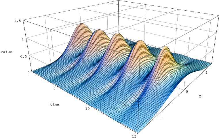
Figure 1: A plot of the function $|\Psi(x,t)|^{2}$, given by Equation (51).

In Fig. (1) we have plotted the probability density given by Eq. (51). Were we have set $\sigma_{0}=\sqrt{\hbar/m\omega}=1$ and $x_{0}=1$.

V A note

Holstein and Swift published a paper in which they presented a cautionary note about the usefulness of the evolution operator method for obtaining the wave function at any future time $t$ from the one at $t=0$ holstein . Notably, in this paper Holstein and Swift showed a particular case where the evolution operator method does not works, but if this case is analyzed by the eigenstates method it works very well. That is to say, the results obtained with both methods do not coincide. Therefore, a contradiction between the evolution operator method and the eigenstates method arise. the goal in this section is to present a solution of this problem.

Firstly, we recall the arguments of reference holstein . In their argumentation, they considered a “free particle” represented by a one-dimensional wave packet described by the function

$$\psi_{H}(x,0) = \exp\left[-a^{2}/\left(a^{2}-x^{2}\right)\right],\quad for\quad\left|x\right|<a$$ (59)

$$= 0,\quad for\quad\left|x\right|\geq a.$$

They argued that $\psi_{H}(x,0)$ is a “good” function because $\psi_{H}(x,0)$ and all its derivatives exist, are continuous for all $x$, and vanish faster than any power as $\left|x\right|\longrightarrow\infty$. When they apply the evolution operator $\exp\left(-\frac{it}{\hbar}\hat{H}\right)$ to the function $\psi_{H}(x,0)$, they found that

$$\sum_{n=0}^{\infty}\left(\frac{i\hbar t}{2m}\right)^{n}\left(n!\right)^{-1}\left(\frac{d^{2}}{dx^{2}}\right)^{n}\psi_{H}(x,0)=0,$$ (60)

when $\left|x\right|>a$ since $\psi_{H}(x,0)$ and all its derivatives vanish for $\left|x\right|>a$. From this result their conclusion was that the particle described by the function $\psi_{H}(x,0)$ is confined within $-a<x<a$ for all time. That is to say, the wave packet does not spread. However, if the problem is solved using the eigenstates method then the wave packet do spread, see reference holstein .

In the next two subsections we analyze this argument from two points of view. In subsection A we analyze it from the mathematical point of view. In the subsection B we give a physical argument.

V.1 Mathematical view

Mathematically, the argument given by Holstein and Swift is well established. From the mathematical point of view, they correctly stated that the function is a well behaved function. That is, because outside of the interval $|x|\geq a$ it vanishes, this function does not have any singularity and, then, it is an analytical function. Therefore, the conclusion is that it is not possible to apply the series of $e^{-it\hat{H}/\hbar}$ to the function $\psi_{H}(x)$. In fact, there is a large set of such function, i. e. $C^{\infty}$, see reference klein .

From this conclusion we can deduce that the evolution operator method fail when one apply it on $\psi_{H}(x)$. This is a very subtle problem. As it was stated in the previous paragraph, the function $\psi_{H}(x)$ is a well behaved function from the mathematical point of view. Therefore, it seems as if the evolution operator method fail when it is applied to an analytical function.

However, after a careful analysis, the only that can be concluded is that the evolution operator method fail for non analytical function. For example, the analysis of J. R. Klein concludes that the evolution operator method hold for $\psi(x,0)$ in a suitable dense subset, see section IV of reference klein . Another possible argument, stated in the following subsection, involves the differences between the Hermitian and self adjoint operators klein and the fact that the particle is free.

Before to give a possible argument, let us recall a similar function studied by Araujo, et. al. araujo . Araujo, et. al., exemplify with the function:

$$u_{ab}=e^{1/(x-a)(x-b)},\quad for\quad a<x<b,$$

$$u_{ab}=0,\quad for\quad 0\leq x\leq a\quad and\quad x\geq b.$$ (61)

For the entire interval, $-\infty<x<\infty$, this function is very similar to the function of Holstein and Swift, $\psi_{H}(x,0)$. However, Araujo, et. al., use the function (61) only to show that the Hamiltonian is not a self-adjoin operator araujo .

V.2 Physical view

In this subsection, we will show that the function used by Holstein and Swift is not a valid physical function in the case of the free particle. A crucial point is that unbounded operators can not be defined on all functions of the Hilbert space klein ; araujo . In order to be able to argue this point, we write the following two explicit assumptions given by the cited authors holstein :

1. The particle is a free particle.

2. The state of the particle at the initial time is given by the function $\psi_{H}(x,0)$.

Our principal point will be that the statements 1) and 2) can not be true at the same time.

We begin analyzing the function from the mathematical point of view in the entire domain of $x$, that is $\left\{x\in R|-\infty\leq x\leq\infty\right\}$, see Fig. (2), where the particle can be found. Notice that the function of Holstein and Swift is defined as zero outside the interval $|x|>a$, therefore, strictly speaking the Fig. (2) is not $\psi_{H}(x)$. However, we use the entire interval $-\infty$ to $+\infty$ because the analysis of reference holstein is for a free particle.

This is a very peculiar function because it has two singularities and many limits:

$$Lim_{x\rightarrow_{-}^{+}\infty}\psi_{H}(x,0)=1,$$

$$Lim_{x\rightarrow a^{+}}\psi_{H}(x,0)=\infty,$$

$$Lim_{x\rightarrow a^{-}}\psi_{H}(x,0)=0,$$

$$Lim_{x\rightarrow-a^{+}}\psi_{H}(x,0)=0,$$

$$Lim_{x\rightarrow-a^{-}}\psi_{H}(x,0)=\infty.$$ (62)

Figure 2: A plot of the function $\psi_{H}(x,0)$.

From the previous equation we can say that the function is not continuous for all $x$ (remember that in this subsection we are studying it in the whole real axe). Furthermore, it does not vanish faster than any power of $x$ as $\left|x\right|\rightarrow\infty$. Therefore, the function is not continuous and $\int_{-\infty}^{\infty}\left|\psi(x)\right|^{2}dx$ is not finite, that is, it is not a square integrable function in the interval $-\infty\leq x\leq\infty$. It is important to stress that we are analyzing the case in which the function has a definite value outside the interval $|x|>a$.

Now, Holstein and Swift holstein define the function as zero in the interval $|x|>a$. With this restriction the function is mathematically a “good” function and can pass as a valid function. That is, as it was stated in the previous subsection, in this case the function does not have the behavior given in Eq. (62). However, one can wonder the next questions: How can the free particle know that it is restricted to the interval $|x|>a$ where the behavior of the function is “good”?, How an state of a physical system can be represented by a function which is mathematically defined as zero outside some interval?

At this point, let us recall the meaning of the wave function in Quantum Mechanics. In the first place, the wave function represents the physical state of a quantum system. That is to say, it represents a combination of the physical properties like energy, momentum, position, etcetera, that can be ascribed to the system. In the second place, $\left|\psi(x,t)\right|^{2}dx$ gives the probability that the particle could be found between $x$ and $dx$. Then, the wave function carries the whole information available for the system. For example, a confined particle is restricted to have certain eigenfunctions that belong to the domain of the Hamiltonian, and certain eigenfunctions that belongs to the domain of the momentum operator araujo ; bonneau ; capri ; gieres , see also reference jordan . The most severe restriction is $\int|\psi(x)|^{2}dx<0$ in the entire interval.

Now, we can give a preliminary answer based in a physical insight to the question quoted in the previous paragraph: How can the free particle know that it is restricted to the interval $|x|\geq a$? By definition, a free particle is a not restricted particle. Therefore, the answer to the question is that there is no way that the particle knows that it is restricted to certain interval, at least if there is not an infinite well where the particle is confined. That is, only in the case of a particle confined in an infinite well we can set the condition $\psi(x,0)=0$ outside of the well, and the Physics changes from that associated to a free particle to that associated to a confined particle garba .

As a conclusion of the previous paragraph, we can state that physically the wave function $\psi_{H}(x,0)$ (when it is defined in the entire interval $-\infty$ to $+\infty$ ) is not valid for the free particle. In fact, the answer is related with the differences between Hermitian and self-adjoint operators. Mathematically, an operator consists of a prescription of operation together with a Hilbert space subset on where the operator is defined klein ; araujo ; bonneau ; gieres . That is, the functions have to belong to the domain of the operator, and if the operator is defined in some interval then the set of functions where the operator is defined, i. e. their domain, have to be defined in the same interval. Therefore, we think that the above example is mistake because the function $\psi_{H}(x,0)$ does not belong to the domain of the hamiltonian operator of the free particle.

Let us explain, the difficulties comes from the fact that in Quantum Mechanics the observable is represented by operators (in a Hilbert space) and the physical states are represented by vectors (wave functions). However, the definitions of both operators and vectors given in most textbooks of Quantum Mechanics are very weak. The majority of them define an operator as an action that changes a vector in another vector, and after that they define Hermitian operators as a symmetric operator. However, there is not any mention about the domain of the operator and the differences between a self-adjoint and Hermitian operators. Because of this weak definition there are many problems or “paradoxes” in the calculations of physical properties, see the examples given in references araujo ; bonneau ; gieres . To handle these problems the concept of self-adjoint extension is reviewed in references araujo ; bonneau ; gieres . Also see references griffiths ; lucio .

Moreover, we adhere the recommendation of Klein klein , Araujo et. al. araujo , Bonneau et. al. bonneau and Gieres gieres : it is necessary to define always the domain of the operators. Therefore, in order to droop up all these problems, we think that it is better to define operators in analogy with the definition of a function. Additionally, it is necessary to clearly state that, as the cited authors have pointed out, unbounded operators cannot be defined on all vectors of the Hilbert space. In particular, it has to be stated that in order that a function can be valid as an initial state it has to be inside of the domain of the hamiltonian $\hat{H}$. On the other hand, the only way to set the condition that a wave function is zero outside of some interval is to collocate an infinite well in that interval.

Therefore, the main point in this subsection is that because the function $\psi_{H}(x,0)$ is not square integrable in the interval $-\infty<x<\infty$, then it does not belong to the domain of the Hamiltonian operator of the free particle. Therefore the function $\psi_{H}(x,0)$ can not represent a state of the free particle. This means that the statements 1) and 2) are not true at same time.

VI conclusion

From the work made in this paper, we can conclude that the evolution operator method is an efficient method to calculate the evolution of a wave function. This method requires, at first instance, the factorization of exponential operators. The factorization allows us to apply the exponential operator individually. We have shown how this method works and apply it in elementary unidimensional cases.

As you may guess, all methods have their troubles and limitations. One trouble of the evolution operator method is that it is not always possible to find the factorization of the exponential operator. Another trouble with this method is that it is not always possible to group the evolving function in a single expression as we show in the Appendix A. However, this method is increasingly used by many authors. For example, we can recall the work of Balasubramanian bala who discussed the time evolution operator method with time dependent Hamiltonians. Also see reference cheng .

Appendix A

Here we show another way to factorize the harmonic oscillator. In this case, we define the function as:

$$F(\xi)=e^{\xi(\hat{A}+\hat{B})}=e^{h(\xi)\hat{C}}e^{f(\xi)\hat{A}}e^{g(\xi)\hat{B}}.$$ (63)

Remember that $\hat{C}=[\hat{A},\hat{B}]$. By differentiating Equation (63) with respect to $\xi$, we obtain:

$$\frac{dF(\xi)}{d\xi}=(\hat{A}+\hat{B})F(\xi),$$ (64)

and

$$\frac{dF(\xi)}{d\xi}=\left[\left(f\frac{dg}{d\xi}+\frac{dh}{d\xi}\right)\hat{C}+e^{2\gamma h(\xi)}\frac{dg}{d\xi}\hat{B}+e^{-2\gamma h(\xi)}\left(\frac{df}{d\xi}+\gamma f^{2}\frac{dg}{d\xi}\right)\hat{A}\right]F(\xi),$$ (65)

By equating Equations (64) and (65), we obtain the following system of differential equations:

$$e^{-2\gamma h(\xi)}\left(\frac{df}{d\xi}+\gamma f^{2}\frac{dg}{d\xi}\right) = 1,$$

$$e^{2\gamma h(\xi)}\frac{dg}{d\xi} = 1,$$

$$f\frac{dg}{d\xi}+\frac{dh}{d\xi} = 0,$$ (66)

subjected to the initial condition:

$$F(0)=1.$$

By solving Equation (66), with the initial condition, we obtain the following solutions:

$$f\left(\xi\right) = \frac{1}{\sqrt{\gamma}}\frac{\tanh\left(\xi\sqrt{\gamma}\right)}{sech^{2}\left(-\xi\sqrt{\gamma}\right)},$$ (67)

$$g\left(\xi\right) = \frac{1}{\sqrt{\gamma}}\tanh\left(\xi\sqrt{\gamma}\right),$$ (68)

$$h\left(\xi\right) = \frac{1}{2\gamma}\ln\left[sech^{2}\left(\xi\sqrt{\gamma}\right)\right],$$ (69)

and we obtain the factorization we were looking for.

A.1 Aplication

The trouble with the factorization given in Eq. (63) is that at some time we have to apply the exponential, which contains the operator $\hat{C}$, of the form:

$$e^{a_{1}xp}e^{x^{2}/4\sigma^{2}},$$ (70)

with $a_{1}$ a constant. The application of this exponential means to apply$\left(xp\right)^{n}\{e^{x^{2}}\}$ which produces the following set of polynomials $A_{n}(x)$ ($n=0,1,2,\dots$):

$${}A_{0} = 1$$

$$A_{1} = 2x^{2}$$

$$A_{2} = 4x^{4}-4x^{2}$$

$$A_{3} = 8x^{6}-24x^{4}+8x^{2}$$

$$A_{4} = 16x^{8}-96x^{6}-112x^{4}+16x^{2}$$ (71)

$$\dots$$

However, we were not able to find the generating function.

References

References

- (1) E. Merzbacher, Quantum Mechanics (Wiley, 1998).
- (2) D. Griffiths, Introduction to Quantum Mechanics (Prentice Hall,1995).
- (3) R. W. Robinett, Quantum Mechanics, Classical Results, Modern Systems, and Visualized Examples (Oxford University Press, 1997).
- (4) S. Gasiorowicz, Quantum Physics (Wiley, 1996).
- (5) B. Holstein, “The harmonic oscillator propagator,” Am. J. Phys. 66 (7), 583-589 (1998).
- (6) F. Gori, D. Ambrosini, R. Borghi, V. Mussi and M. Santarsiero, “The propagator for a particle in a well,” Eur. J. Phys. 22, 53 66 (2001).
- (7) Barone et al. ‘Three methods for calculating the Feynman propagator,” Am. J. Phys. 71, 483-491 (2003).
- (8) K. Kumar, “Expansion of a function of noncommuting operators,” Jour. Mathem. Phys. 6, 1923 (1965).
- (9) L. Cohen,“Expansion theorem for functions operators,” Jour. Mathem. Phys. 7, 244 (1966).
- (10) S. M. Blinder “Evolution of Gaussian wavepacket,” Am. J. Phys. 36 525 (1968).
- (11) R. W. Robinett, “Quantum mechanical time-development operator for the uniformly accelerated particle” Am. J. Phys. 64 803 (1996).
- (12) S. Balasubramanian, “Time-development operator method in quantum mechanics,” Am. J. Phys. 69 (4), 508-511 (2001).
- (13) C. M. Cheng and P. C. W. Fun, “The evolution operator technique in solving the Schrödinger equation, and its applications to disentangling exponential operators and solving the problem of mass-varing harmonic oscillator,” J. Phys. A: Math. Gen. 21, 4115-4131 (1988).
- (14) P. C. García Quijas and L. M. Arévalo Aguilar, “Overcoming misconceptions in Quantum Mechanics with the time evolution operator,” to be publised elsewhere.
- (15) R. M. Wilcox, “Exponential operator and parameter differentiation in Quantum Physics,” Jour. Mathem. Phys. 8, 962 (1967).
- (16) W. H. Louisell, Quantum statistical Properties of Radiation (John Wiley, 1990) Chap. 3.
- (17) M. Lutzky, “Parameter differentiation of exponential operators an the Baker-Campbell-Hausdorff formula,” Jour. Mathem. Phys. 9, 1125 (196).
- (18) L. M. Arévalo Aguilar and H. Moya-Cessa, “Solution to the Master Equation for Quantized Cavity Mode,” Quantum Semiclass. Opt. 10, 671 (1998).
- (19) A. Vidiella-Barranco, L. M. Arévalo-Aguilar y H. Moya-Cessa “Analytical operator solution of master equations describing phase-sensitive processes,” International Journal of Modern Physics B 15, 1127-1134 (2001).
- (20) Huai-Xin Lu, Jie Yang, Yong-De Zhang, and Zeng-Bing Chen, “Algebraic approch to master equations with superoperator generators of su(1,1) and su(2) Lie algebras,” Phys. Rev. A 67, 024101 (2003).
- (21) C. Singh, M. Belloni, and W. Christian, “Improving Students’ understanding of quantum mechanics,” Physics Today 59, 43 august (2006).
- (22) L. A. Beauregard, “Time evolution operator for the Harmonic Oscillator,” Am. J. Phys. 33, 1084 (1965).
- (23) B. R. Holstein and A. R. Swift, “Spreading Wave Packets-A Cautionay Note,” Am. J. Phys. 40 829-832 (1972).
- (24) J. R. Klein, “Do free quantum-mechanical wave packets always spread?,” Am. J. Phys. 48 1035-1037 (1972).
- (25) V. S. Araujo, F. A. B. Coutinho and J. F. Perez “Operator domains and self-adjoint operators,” Am. J. Phys. 72 (2), 203-213 (2004).
- (26) G. Bonneau, J. Faraut and G. Valent “Selft-adjoint extensions of operators and the teaching of quantum mechanics,” Am. J. Phys. 69 (3), 322-331 (2001).
- (27) A. Z. Capri, “Selft-adjointness and spontaneously broken symmetry,” Am. J. Phys. 45, 823-825 (1977).
- (28) F. Gieres, “Mathematical surprises and Dirac’s formalism in quantum mechanics,” arXiv:quant-ph/9907069.
- (29) T. F. Jordan,“Conditions on wave functions derived from operator domains,” Am. J. Phys. 44 (6), 567-570 (1976).
- (30) For a different interpretation see the work of Garbaczewski and Karwowski, P. Garbaczewski and W. Karwowski, “Impenetrable barriers and canonical quantization,” Am. J. Phys. 72 (7), 924-933 (2004).
- (31) A. M. Essin and D. J. Griffiths,“Quantum mechanics of the poterntial,” Am. J. Phys. 74 (2), 109-117 (2006).
- (32) A. Cabo, J. L. Lucio, and H. Mercado,“On scale invariance and anomalies in quantum mechanics,” Am. J. Phys. 66 (3), 240-246 (1997).