Hypothesis testing for an entangled state produced
by spontaneous parametric down conversion

Abstract

Generation and characterization of entanglement are crucial tasks in quantum information processing. A hypothesis testing scheme for entanglement has been formulated. Three designs were proposed to test the entangled photon states created by the spontaneous parametric down conversion. The time allocations between the measurement vectors were designed to consider the anisotropic deviation of the generated photon states from the maximally entangled states. The designs were evaluated in terms of the p-value based on the observed data. It has been experimentally demonstrated that the optimal time allocation between the coincidence and anti-coincidence measurement vectors improves the entanglement test. A further improvement is also experimentally demonstrated by optimizing the time allocation between the anti-coincidence vectors. Analysis on the data obtained in the experiment verified the advantage of the entanglement test designed by the optimal time allocation.

I Introduction

The concept of entanglement has been thought to be the heart of quantum mechanics. The seminal experiment by Aspect et al. APG82 has proved the ’spooky’ non-local action of quantum mechanics by observing violation of Bell inequality Bell93 with entangled photon pairs. Recently, entanglement has been also recognized as an important resource for quantum information processing, explicitly or implicitly. For example, entanglement provides an exponential speed-up in some computational tasks Shor97 , and unconditional security in cryptographic communications SP00 . A hidden entanglement between the legitimate parties guarantees the security in BB84 quantum cryptographic protocol SP00 ; BB84 . Quantum communication between arbitrarily distant parties has been shown to be possible by a quantum repeater Briegel98 based on quantum teleportation Bennett93 . Practical realization of entangled states is therefore one of the most important issues in the quantum information technology.

The practical implementation raises a problem to verify the amount of entanglement. A quantum information protocol requires a minimum entanglement. It is, however, not always satisfied in actual experiments. Unavoidable imperfections will limit the entanglement in generation process. Moreover, decoherence and dissipation due to the coupling with the environment will degrade the entanglement during the processing. Therefore, it is a crucial issue to characterize the entanglement of the generated (or stored) states to guarantee the successful quantum information processing. For this purpose, quantum state estimation and Quantum state tomography are known as a method of identifying the unknown state Selected ; helstrom ; holevo . Quantum state tomography WJEK99 has recently applied to obtain full information of the $4\times 4$ two-particle density matrix from the coincidence counts of 16 combinations of measurement usami . However, characterization is not the goal of an experiment, but only a part of preparation. It is thus favorable to reduce the time for characterization and the number of consumed particles as possible. An entanglement test, which should be simpler than the full characterization, works well in most applications, because we only need to know whether the states are sufficiently entangled or not. We can reduce the resources for characterization with the entanglement test. Barbieri et al. BMNMDM03 introduced an entanglement witness to test the entanglement of polarized entangled photon pairs. Tsuda et al. TMH05 studied the optimization problem on the entanglement tests with the mathematical statistics in the POVM framework. Hayashi et al. HTM treated this optimization problem in the framework of Poisson distribution, which describes the stochastic behavior of the measurement outcomes on the two-photon pairs generated by spontaneous parametric down conversion (SPDC).

In this paper, we will apply the experimental designs proposed in ref. HTM to test the polarization entangled two-photon pairs generated by SPDC. The two-photon states can be characterized by the correlation of photon detection events in several measurement bases. In experiments, the correlation is measured by coincidence counts of photon detections on selected polarizations. The coincidence counts on a combination of the two from horizontal ($H$), vertical ($V$), $45^{\circ}$ linear ($X$), $135^{\circ}$ linear ($D$), clock-wise circular ($R$), and anti-clock-wise circular ($L$) polarizations defines a measurement vector. We here use the same representations for the measurement vectors as the state vectors, such as $|HH\rangle$. If the state is close to $|\Phi^{(+)}\rangle=\frac{1}{\sqrt{2}}(|HH\rangle+|VV\rangle)$, the coincidence counts on the vectors $|HH\rangle,|VV\rangle,|DD\rangle,|XX\rangle,|RL\rangle,$ and $|LR\rangle$ yield the maximum values, whereas the counts on the vectors $|HV\rangle,|VH\rangle,|DX\rangle,|XD\rangle,|RR\rangle,$ and $|LL\rangle$ take the minimum values. We will refer to the former vectors as the coincidence vectors, and to the latter as the anti-coincidence vectors. The ratio of the minimum counts to the maximum counts measures the degree of entanglement. In the following sections, we formulate the hypothesis testing of entanglement in the view of statistics. We then improve the test by optimizing the allocation on the measurement time for each measurement, considering that the counts on the anti-coincidence vectors are much smaller than those on the coincidence vectors.

The test can be further improved, if we utilize the knowledge on the tendency of the entanglement degradation. In general, the error from the maximally entangled states can be anisotropic, which reflects the generation process of the states. We can improve the sensitivity to the entanglement degradation by focusing the measurement on the expected error directions. In the present experiment, we generated polarization entangled photon pairs from a stack of two type-I phase matched nonlinear crystals KWWAE99 ; NUTMK02 , where one nonlinear crystal generates a photon pair polarized in the horizontal direction $(|HH\rangle)$, and the other generates a photon pair polarized in the vertical direction $(|VV\rangle)$. If the two pairs are indistinguishable, the generated photons are entangled in a two-photon state $\frac{1}{\sqrt{2}}(|HH\rangle+\exp[i\delta]|VV\rangle)$. Otherwise, the state will be a mixture of $HH$ pairs and $VV$ pairs. The quantum state tomography has shown that the only $HHHH$, $VVVV$, $VVHH$, $HHVV$ elements are dominant NUTMK02 , which implies that the density matrix can be approximated by a classical mixture of $|\Phi^{(+)}\rangle\langle\Phi^{(+)}|$ and $|\Phi^{(-)}\rangle\langle\Phi^{(-)}|$. We can improve the entanglement test on the basis of this property, as described in the following sections.

The construction of this article is following. Section II gives the mathematical formulation concerning statistical hypothesis testing. Section III defines the hypothesis scheme for the entanglement of the two-photon states generated by SPDC. Sections IV - VII describe testing methods as well as design of experiment. Section VIII examines the experimental aspects of the hypothesis testing on the entanglement. The designs on the time allocation are evaluated by the experimental data.

II Hypothesis testing for probability distributions

II.1 Formulation

In this section, we review the fundamental knowledge of hypothesis testing for probability distributionslehmann . Suppose that a random variable $X$ is distributed according to a probability measure $P_{\theta}$ identified by an unknown parameter $\theta$, and that the unknown parameter $\theta$ belongs to one of the mutually disjoint sets $\Theta_{0}$ and $\Theta_{1}$. When the task is to guarantee that the true parameter $\theta$ belongs to the set $\Theta_{1}$ with a certain significance, we choose the null hypothesis $H_{0}$ and the alternative hypothesis $H_{1}$ as

$$H_{0}:\theta\in\Theta_{0}\mbox{ vs. }H_{1}:\theta\in\Theta_{1}.$$ (1)

The task is then described by a test, where we decide to accept the hypothesis $H_{1}$ by rejecting the null hypothesis $H_{0}$ with confidence. We make no decision when we can not reject the null hypothesis. The test based is characterized as a function $\phi(x)$ taking a value in $\{0,1\}$; we can reject $H_{0}$ if $\phi(x)=1$, but can not reject it if $\phi(x)=0$. The test can be also described by the rejection region defined by $\{x|\phi(x)=1\}$, whether the data $x$ falls into the rejection region or not. The function $\phi(x)$ should be designed properly according to the problem to provide an appropriate test.

For example, suppose that mutually independent data $x_{1},\cdots,x_{n}$ obey a normal distribution with unknown mean $\mu$ and known variance $\sigma_{0}^{2}$

$$P_{\mu}(x)=\frac{1}{\sqrt{(2\pi\sigma_{0}^{2})^{n}}}\exp\left[-\frac{\sum_{i=1}^{n}(x_{i}-\mu)^{2}}{2\sigma_{0}^{2}}\right].$$ (2)

We introduce a hypothesis testing

$$H_{0}:\mu\in\{\mu|\mu\leq\mu_{0}\}\mbox{ vs. }H_{1}:\mu\in\{\mu|\mu>\mu_{0}\}$$ (3)

to decide the mean is larger than a value $\mu_{0}$ with a confidence level $\alpha$. Then the function $\phi$ of the average on the data is defined by $\bar{x}=(1/n)\sum_{i=1}^{n}x_{i}$ as

$$\phi(x)=\left\{\begin{array}[]{ll}&1,\>\mbox{ if }\sqrt{n}(\bar{x}-\mu_{0})/\sigma_{0}>z_{\alpha}\\ &0,\>\mbox{ if }\sqrt{n}(\bar{x}-\mu_{0})/\sigma_{0}\leq z_{\alpha},\end{array}\right.$$ (6)

where $z_{\alpha}$ is given by

$$z_{\alpha} =\Phi^{-1}(\alpha)$$ (7)

$$\Phi(z) :=\int_{-\infty}^{z}\frac{1}{\sqrt{2\pi}}e^{-\frac{y^{2}}{2}}dy.$$ (8)

The rejection region is provided as

$$\{x|\sqrt{n}(\bar{x}-\mu_{0})/\sigma_{0}>z_{\alpha}\}$$ (9)

in this test.

II.2 p-values

In a usual hypothesis testing, we fix our test before applying it to the data. Sometimes, however, we compare tests in a class $T$ by the minimum risk probability to reject the hypothesis $H_{0}$ with given data. This probability is called the p-value, which depends on the observed data $x$ as well as the subset $\Theta_{0}$ to be rejected. For a given class $T$ of tests, the p-value is defined as

$$pval:=\min_{\phi\in T:\phi(x)=1}\max_{\theta\in\Theta_{0}}P_{\theta}(\phi).$$ (10)

In the hypothesis test for a normal distribution defined previously (Eqs. (2)-(8)), the p-value is given by

$$pval=\Phi(\sqrt{n}(\bar{x}-\mu_{0})/\sigma_{0}).$$ (11)

The concept of p-value is useful for comparison of several designs of experiment.

II.3 Likelihood Test

In mathematical statistics, the likelihood ratio tests is often used as a class of standard testslehmann . Likelihood is a function of unknown parameter $\theta$ defined as the probability distribution $P_{\theta}(x)$ for given data $x$. When both $\Theta_{0}$ and $\Theta_{1}$ consist of single elements as $\Theta_{0}=\{\theta_{0}\}$ and $\Theta_{1}=\{\theta_{1}\}$, the rejection region of the likelihood ratio test is defined as

$$\left\{x\left|\frac{P_{\theta_{0}}(x)}{P_{\theta_{1}}(x)}<r\right.\right\}.$$

where $r$ is a constant, and the ratio $P_{\theta_{0}}(x)/P_{\theta_{1}}(x)$ is called the likelihood ratio. In the general case, i.e., the cases where $\Theta_{0}$ or $\Theta_{1}$ has at least two elements, the likelihood ratio test is given by its rejection region:

$$\left\{x\left|\frac{\sup_{\theta\in\Theta_{0}}P_{\theta}(x)}{\sup_{\theta\in\Theta_{1}}P_{\theta}(x)}<r\right.\right\}.$$

In the hypothesis test for a normal distribution defined previously (Eqs. (2)-(8)), logarithm of the likelihood ratio is given by

$$\log\frac{P_{\mu_{0}}(x)}{P_{\bar{\mu}=\bar{x}}(x)} =\frac{1}{2\sigma_{0}^{2}}\left\{\sum\left(x_{i}-\mu_{0}\right)^{2}-\sum\left(x_{i}-\bar{\mu}\right)^{2}\right\}$$

$$=\hbox to0.0pt{$\displaystyle-\frac{n(\bar{x}-\mu_{0})^{2}}{2\sigma_{0}^{2}}$\hss}.$$ (12)

Therefore, the rejection region of the likelihood ratio test coincide with Eq. (9), if we set $r=\exp[-z_{\alpha}^{2}/2]$.

III Hypothesis Testing scheme for entanglement in SPDC experiments

III.1 Formalization

This section introduces the hypothesis test for entanglement. We consider the entanglement of two-photon pairs generated by SPDC. The two-photon state is described by a density matrix $\sigma$. We assume two-photon generation process to be identical but individual. Here we measure the entanglement by the fidelity between the generated state $\sigma$ and the maximally entangled target state $|\Phi^{(+)}\rangle$:

$$F=\langle\Phi^{(+)}|\sigma|\Phi^{(+)}\rangle.$$ (13)

The purpose of the test is to guarantee, with a certain significance, that the state is sufficiently close to the maximally entangled state. For this purpose, the hypothesis that the fidelity $F$ is less than a threshold $F_{0}$ should be disproved with a small error probability. In mathematical statistics, the above situation is formulated as hypothesis testing; we introduce the null hypothesis $H_{0}$ that entanglement is not enough and the alternative $H_{1}$ that the entanglement is enough:

$$H_{0}:F\leq F_{0}\hbox{ vs. }H_{1}:F>F_{0},$$ (14)

with a threshold $F_{0}$.

The coincidence counts of photon pairs generated in the SPDC experiments can be assumed to be a random variable independently distributed according to a Poisson distribution. In the following, a symbol labeled by a pair $(x,y)$ represents a random variable or parameter related to the measurement vectors $|x,y\rangle$. When the dark count is negligible, the number of detection events (i.e., coincidence counts) $n_{xy}$ on the vectors $|x,y\rangle$ is a random variable according to the Poisson distribution ${\rm Poi}(\lambda\mu_{xy}t_{xy})$ of mean $\lambda\mu_{xy}t_{xy}$, where

• $\lambda$ is a known constant related to the photon detection rate, determined from the averaged photon-pair-generation rate and the detection efficiency,

• $\mu_{xy}=\langle x,y|\sigma|x,y\rangle$ is an unknown constant,

• $t_{xy}$ is a known constant of the time for detection.

The probability function of $n_{xy}$ is

$$n_{xy}={\rm Poi}(\lambda\mu_{xy}t_{xy})=\exp(-\lambda\mu_{xy}t_{xy})\frac{(\lambda\mu_{xy}t_{xy})^{n_{xy}}}{n_{xy}!}.$$

Because the detections at different times are mutually independent, $n_{xy}$ is independent of $n_{x^{\prime}y^{\prime}}$ ($x\neq x^{\prime}$ or $y\neq y^{\prime}$). In this paper, we discuss the quantum hypothesis testing under the above assumptions, whereas Usami et al.usami discussed the state estimation under the same assumptions.

III.2 Modified visibility

Visibility of the two-photon interference is an indicator of entanglement commonly used in the experiments. The two-photon interference fringe is obtained by the measurement of coincidence counts on the vector $|x,y\rangle$, where the vector $|y\rangle$ is rotated along a great circle on the Poincare sphere with a fixed vector $|x\rangle$. The visibility is calculated with the maximum and minimum number of coincidence counts, $n_{max}$ and $n_{min}$, as the ratio $(n_{max}-n_{min})/(n_{max}+n_{min})$. We need to make the measurement with at least two fixed vectors $|x\rangle$ in order to exclude the possibility of the classical correlation. We may choose the two vectors $|H\rangle$ and $|D\rangle$ as $|x\rangle$, for example. However, our decision will contain a bias, if we measure the coincidence counts only with two fixed vectors. The bias in the measurement emerges as the fact that the visibility reflects not only the fidelity but also the direction of the deviation of the given state from the maximally entangled target state. Hence, we cannot estimate the fidelity in a statistically proper way from the visibility.

In order to remove the bias based on such a direction, we propose to measure the counts on the coincidence vectors $|HH\rangle,|VV\rangle,|DD\rangle,|XX\rangle,|RL\rangle,$ and $|LR\rangle$, and the counts of the anti-coincidence vectors $|HV\rangle,|VH\rangle,|DX\rangle,|XD\rangle,|RR\rangle$, and $|LL\rangle$. The former corresponds to the maximum coincidence counts in the two-photon interference, and the latter does to the minimum. Since the equations

$$|HH\rangle\langle HH|+|VV\rangle\langle VV|+|DD\rangle\langle DD|$$

$$+|XX\rangle\langle XX|+|RL\rangle\langle RL|+|LR\rangle\langle LR|$$

$$= 2|\Phi^{(+)}\rangle\langle\Phi^{(+)}|+I$$ (15)

and

$$|HV\rangle\langle HV|+|VH\rangle\langle VH|+|XD\rangle\langle XD|$$

$$+|DX\rangle\langle DX|+|RR\rangle\langle RR|+|LL\rangle\langle LL|$$

$$= 2I-2|\Phi^{(+)}\rangle\langle\Phi^{(+)}|$$ (16)

hold, In this paper, we call this proposed method the modified visibility method. Using this method, we can test the fidelity between the maximally entangled state $|\Phi^{(+)}\rangle\langle\Phi^{(+)}|$ and the given state $\sigma$, using the total number of counts of the coincidence events (the total count on coincidence event) $n_{1}$ and the total number of counts of the anti-coincidence events (the total count on anti-coincidence events) $n_{2}$ obtained by measuring on all the vectors with the time $\frac{t}{12}$. holds, we can estimate the fidelity by measuring the sum of the counts of the following vectors: $|HH\rangle,|VV\rangle,|DD\rangle,|XX\rangle,|RL\rangle,$ and $|LR\rangle$, when $\lambda$ is knownBMNMDM03 ; TMH05 . This is because the sum $n_{1}:=n_{HH}+n_{VV}+n_{DD}+n_{XX}+n_{RL}+n_{LR}$ obeys the Poisson distribution with the expectation value $\lambda\frac{1+2F}{6}t_{1}$, where the measurement time for each vector is $\frac{t_{1}}{6}$. We call these vectors the coincidence vectors because these correspond to the coincidence events.

However, since the parameter $\lambda$ is usually unknown, we need to perform another measurement on different vectors to obtain additional information. also holds, we can estimate the fidelity by measuring the sum of the counts of the following vectors: $|HV\rangle,|VH\rangle,|DX\rangle,|XD\rangle,|RR\rangle$, and $|LL\rangle$. The sum $n_{2}:=n_{HV}+n_{VH}+n_{DX}+n_{XD}+n_{RR}+n_{LL}$ obeys the Poisson distribution $\rm Poi(\lambda\frac{2-2F}{6}t_{2})$, where the measurement time for each vector is $\frac{t_{2}}{6}$. Combining the two measurements, we can estimate the fidelity without the knowledge of $\lambda$. We call these vectors the anti-coincidence vectors because these correspond to the anti-coincidence events.

We can also consider different type of measurement on $\lambda$. If we prepare our device to detect all photons, the detected number $n_{3}$ obeys the distribution $\rm Poi(\lambda t_{3}$) with the measurement time $t_{3}$. We will refer to it as the total flux measurement. In the following, we consider the best time allocation for estimation and test on the fidelity, by applying methods of mathematical statistics. We will assume that $\lambda$ is known or estimated from the detected number $n_{3}$.

IV Modification of Visibility

The total count on coincidence events $n_{1}$ obeys Poi$(\lambda\frac{2F+1}{12}t)$, and the count on total anti-coincidence events $n_{2}$ obeys the distribution Poi$(\lambda\frac{2-2F}{12}t)$. These expectation values $\mu_{1}$ and $\mu_{2}$ are given as $\mu_{1}=\lambda\frac{2F+1}{12}t$ and $\mu_{2}=\lambda\frac{2-2F}{12}t$. Since the ratio $\frac{\mu_{2}}{\mu_{1}+\mu_{2}}$ is equal to $\frac{2}{3}(1-F)$, we can estimate the fidelity using the ratio $\frac{n_{2}}{n_{1}+n_{2}}$ as $\hat{F}(n_{1},n_{2})=1-\frac{3}{2}\frac{n_{2}}{n_{1}+n_{2}}$. Its variance is asymptotically equal to

$$\frac{1}{\lambda(\frac{t}{3(2F+1)}+\frac{t}{3(2-2F)})}=\frac{(2F+1)(2-2F)}{\lambda t}.$$ (17)

Hence, similarly to the visibility, we can check the fidelity by using this ratio.

Indeed, when we consider the distribution under the condition that the total count $n_{1}+n_{2}$ is fixed to $n$, the random variable $n_{2}$ obeys the binomial distribution with the average value $\frac{2}{3}(1-F)n$. Hence, we can apply the likelihood test of the binomial distribution. In this case, by the approximation to the normal distribution, the likelihood test with the risk probability $\alpha$ is almost equal to the test with the rejection region concerning the null hypothesis $H_{0}:F\leq F_{0}$: $\{(n_{1},n_{2})|\frac{n_{2}}{n_{1}+n_{2}}\leq\frac{2}{3}(1-F_{0})+\Phi^{-1}(\alpha)\sqrt{\frac{(2-2F_{0})(1+2F_{0})}{9(n_{1}+n_{2})}}\}$, where $\Phi(\alpha):=\int_{-\infty}^{\alpha}\frac{1}{\sqrt{2\pi}}e^{-\frac{x^{2}}{2}}dx$. The p-value of this kind of tests is $\Phi(\frac{n_{2}(2F_{0}+1)-n_{1}(2-2F_{0})}{\sqrt{(n_{1}+n_{2})(2F_{0}+1)(2-2F_{0})}})$.

V Design I ($\lambda$: unknown, One-Stage)

In this section, we consider the problem of testing the fidelity between the maximally entangled state $|\Phi^{(+)}\rangle\langle\Phi^{(+)}|$ and the given state $\sigma$ by performing three kinds of measurement, coincidence, anti-coincidence, and total flux, with the times $t_{1},t_{2}$ and $t_{3}$, respectively. The data $(n_{1},n_{2},n_{3})$ obeys the multinomial Poisson distribution Poi$(\lambda\frac{2F+1}{6}t_{1},\lambda\frac{2-2F}{6}t_{2},\lambda t_{3})$ with the assumption that the parameter $\lambda$ is unknown. In this problem, it is natural to assume that we can select the time allocation with the constraint for the total time $t_{1}+t_{2}+t_{3}=t$.

As is shown in Hayashi et al HTM , when $F_{1}:=0.899519\leq F\leq 1$, the minimum variance of the estimator is asymptotically equal to $\frac{(1-F)(\sqrt{3}+\sqrt{1-F})^{2}}{\lambda t}$, which is attained by the optimal time allocation $t_{1}=0$, $t_{2}=\frac{\sqrt{3}}{(\sqrt{3}+\sqrt{1-F})}t$, $t_{3}=\frac{\sqrt{1-F}}{\sqrt{3}+\sqrt{1-F}}t$. Otherwise, it is asymptotically equal to $\frac{(2F+1)(1-F)(\sqrt{2F+1}+\sqrt{2-2F})^{2}}{3\lambda t}$, which is attained by the optimal time allocation $t_{1}=\frac{\sqrt{2-2F}}{\sqrt{2F+1}+\sqrt{2-2F}}t$, $t_{2}=\frac{\sqrt{2F+1}}{\sqrt{2F+1}+\sqrt{2-2F}}t$, $t_{3}=0$. This optimal asymptotic variance is much better than that obtained by the modified visibility method.

Since the optimal allocation depends only on the true parameter $F$, it is suitable to choose the optimal time allocation at the threshold $F_{0}$ for testing whether the fidelity is greater than the threshold $F_{0}$. In the both cases, when we perform the optimal allocation, the data obeys the binomial Poisson distribution. Hence, similarly to the modified visibility, we can check the fidelity by applying the likelihood test of binomial distribution to the ratio between two kinds of counts.

In the former case, the likelihood test with the risk probability $\alpha$ is almost equal to the test with the rejection region $H_{0}:F\leq F_{0}$: $\{(n_{2},n_{3})|\frac{n_{2}}{n_{2}+n_{3}}\leq\frac{\sqrt{1-F_{0}}}{\sqrt{3}+\sqrt{1-F_{0}}}+\frac{\Phi^{-1}(\alpha)}{\sqrt{3}+\sqrt{1-F_{0}}}\sqrt{\frac{\sqrt{1-F_{0}}\sqrt{3}}{n_{2}+n_{3}}}\}$. The p-value of this kind of tests is $\Phi(\frac{n_{2}\sqrt{3}-n_{3}\sqrt{1-F_{0}}}{\sqrt{(n_{2}+n_{3})\sqrt{1-F_{0}}\sqrt{3}}})$. In the later case, the likelihood test with the risk probability $\alpha$ is almost equal to the test with the rejection region concerning the null hypothesis $H_{0}:F\leq F_{0}$: $\{(n_{1},n_{2})|\frac{n_{2}}{n_{2}+n_{1}}\leq\frac{\sqrt{2-2F_{0}}}{\sqrt{2F_{0}+1}+\sqrt{2-2F_{0}}}+\frac{\Phi^{-1}(\alpha)}{\sqrt{2F_{0}+1}+\sqrt{2-2F_{0}}}\sqrt{\frac{\sqrt{2-2F_{0}}\sqrt{2F_{0}+1}}{n_{1}+n_{2}}}\}$. The p-value of this kind of tests is $\Phi(\frac{n_{2}\sqrt{2F_{0}+1}-n_{1}\sqrt{2-2F_{0}}}{\sqrt{(n_{1}+n_{2})\sqrt{2F_{0}+1}\sqrt{2-2F_{0}}}})$.

VI Design II ($\lambda$: known, One-Stage)

In this section, we consider the case where $\lambda$ is known. In this case, when $F\geq\frac{1}{4}$, the optimal time allocation is $t_{2}=t$, $t_{1}=t_{3}=0$. That is, the count on anti-coincidence $(t_{1}=0;t_{2}=t)$ is better than the count on coincidence $(t_{1}=t;t_{2}=0)$. In fact, Barbieri et al.BMNMDM03 measured the sum of the counts on the anti-coincidence vectors $|HV\rangle,|VH\rangle,|DX\rangle,|XD\rangle,|RR\rangle,|LL\rangle$ to realize the entanglement witness in their experiment. In this case, the count on anti-coincidence $n_{2}$ obeys the Poisson distribution with the average $\lambda\frac{1-F}{3}t$, the fidelity is estimated by $1-\frac{3n_{1}}{\lambda t}$. Its variance is $\frac{3(1-F)}{\lambda t}$. Then, the likelihood test with the risk probability $\alpha$ of the Poisson distribution is almost equal to the test with the rejection region: $\{n_{2}|n_{2}\leq\frac{\lambda(1-F_{0})}{3}t+\Phi^{-1}(\alpha)\sqrt{\frac{\lambda(1-F_{0})}{3}t}\}$ concerning the null hypothesis $H_{0}:F\leq F_{0}$. The p-value of likelihood tests is $\Phi(\frac{n_{2}-\lambda(1-F_{0})t/3}{\sqrt{\lambda(1-F_{0})t/3}})$.

When $F<\frac{1}{4}$, the optimal time allocation is $t_{1}=t$, $t_{2}=t_{3}=0$. The fidelity is estimated by $\frac{3n_{2}}{\lambda t}-\frac{1}{2}$. Its variance is $\frac{3(1+2F)}{2\lambda t}$. Then, the likelihood test with the risk probability $\alpha$ of the Poisson distribution is almost equal to the test with the rejection region: $\{n_{1}|n_{1}\geq\lambda\frac{1+2F_{0}}{6}t+\Phi^{-1}(1-\alpha)\sqrt{\lambda\frac{1+2F_{0}}{6}t}\}$ concerning the null hypothesis $H_{0}:F\leq F_{0}$. The p-value of likelihood tests is $\Phi(\frac{-n_{1}+\lambda(1+2F_{0})t/6}{\sqrt{\lambda(1+2F_{0})t/6}})$.

VII Design III ($\lambda$: known, Two-Stage)

Next, for a further improvement, we minimize the variance by optimizing the time allocation $t_{HV}$, $t_{VH}$, $t_{DX}$, $t_{XD}$, $t_{RR}$, and $t_{LL}$ between the anti-coincidence vectors $B=\{|HV\rangle$, $|VH\rangle$, $|DX\rangle$, $|XD\rangle$, $|RR\rangle$, $|LL\rangle\}$, respectively, under the restriction of the total measurement time: $t_{HV}+t_{VH}+t_{DX}+t_{XD}+t_{RR}+t_{LL}=t$. The number of the counts $n_{xy}$ obeys Poisson distribution Poi($\lambda\mu_{xy}t_{xy}$) with the unknown parameter $\mu_{xy}=\langle x_{A}y_{B}|\sigma|x_{A}y_{B}\rangle$. the minimum value of estimation of the fidelity $F=1-\frac{1}{2}\sum_{(x,y)\in B}\mu_{xy}$ is

$$\frac{(\sum_{(x,y)\in B}\sqrt{\mu_{x,y}})^{2}}{4\lambda t},$$ (18)

which is attained by the optimal time allocation

$$t_{xy}=\frac{\sqrt{\mu_{xy}}t}{\sum_{(x,y)\in B}\sqrt{\mu_{x,y}}},$$ (19)

which is called Neyman allocation and is used in sampling designCochran .

However, this optimal time allocation is not applicable in the experiment, because it depends on the unknown parameters $\mu_{HV},$ $\mu_{VH},$ $\mu_{DX},$ $\mu_{XD},$ $\mu_{RR},$ and $\mu_{LL}$. In order to resolve this problem, we use a two-stage method, where the total measurement time $t$ is divided into $t_{f}$ for the first stage and $t_{s}$ for the second stage under the condition of $t=t_{f}+t_{s}$. In the first stage, we measure the counts on the anti-coincidence vectors for $t_{f}/6$ and estimate the expectation value for Neyman allocation on measurement time $t_{s}$. In the second stage, we measure the counts on anti-coincidence vectors $|x_{A}y_{B}\rangle$ according to the estimated Neyman allocation. The two-stage method is formulated as follows.
(i) The measurement time for each vector in the first stage is given by $t_{f}/6$
(ii) In the second stage, we measure the counts on a vector $|x_{A}y_{B}\rangle$ the measurement time $\tilde{t}_{xy}$ defined as

$$\tilde{t}_{xy}=\frac{m_{xy}}{\sum_{(x,y)\in B}\sqrt{m_{xy}}}(t-t_{f})$$

where $m_{xy}$ is the observed count in the first stage.
(iii) Define $\hat{\mu}_{xy}$ and $\hat{F}$ as

$$\hat{\mu}_{xy}=\frac{n_{xy}}{\lambda\tilde{t}_{xy}},\quad\hat{F}=1-\frac{1}{2}\sum_{(x,y)\in B}\hat{\mu}_{x,y},$$

where $n_{x,y}$ is the number of the counts on $|x_{A}y_{B}\rangle$ for $\tilde{t}_{xy}$. Then, we can estimate the fidelity by $\hat{F}$.

We can test our hypothesis by using the likelihood test, which has the rejection region:

$$\left\{\vec{n}\left|\sup_{\vec{\mu}\cdot\vec{w}\geq c_{0}}{\rm Poi}(\vec{\mu})(\vec{n})\leq r\sup_{\vec{\mu}\cdot\vec{w}<c_{0}}{\rm Poi}(\vec{\mu})(\vec{n})\right.\right\},$$

where $w_{i}:=\frac{1}{2\lambda\tilde{t}_{i}}$ and $c_{0}:=1-F_{0}$. However, it is very difficult to choose $r$ such that the likelihood test has a given risk probability $\alpha$. In order to resolve this problem, Hayashi et al. HTM proposed a better method. For treating this method, we number the anti-coincidence vectors by $i=1,\ldots,6$. Then, the rejection region with the risk probability $\alpha$ is given by ${\cal B}_{R_{\alpha}}$, where the set ${\cal B}_{R}$ is defined by

$${\cal B}_{R}:=\left\{\vec{n}^{\prime}\left|\sum_{i=1}^{6}\frac{n_{i}^{\prime}}{\tilde{\mu}_{i}(R)}\leq 1\right.\right\},$$ (20)

and $\tilde{\mu}_{i}(R)$ are defined as follows:

$$\frac{c_{0}}{w_{i}}-\tilde{\mu}_{i}(R)+\tilde{\mu}_{i}(R)\log\frac{\tilde{\mu}_{i}(R)w_{i}}{c_{0}} =R\hbox{~{}~{}if }R\leq R_{0,i}$$ (21)

$$\frac{c_{0}}{w_{M}}+\tilde{\mu}_{i}(R)\log\frac{w_{M}-w_{i}}{w_{M}} =R\hbox{~{}~{}if }R>R_{0,i}$$ (22)

where $w_{M}:=\max_{i}w_{i}$ and $R_{0,i}:=\frac{c_{0}}{w_{M}}+\frac{c_{0}(w_{M}-w_{i})}{w_{i}w_{M}}\log\frac{w_{M}-w_{i}}{w_{M}}$. The value $R_{\alpha}$ is defined by

$$-\min_{i\neq j}z_{i,j}(R_{\alpha})=\Phi^{-1}(\alpha),$$ (23)

where $z_{i,j}(R)$ is given by

$$z_{i,j}(R):=\left\{\begin{array}[]{ll}\frac{x_{i}(R)}{\sqrt{y_{i}(R)}}&\hbox{ if }\frac{2x_{j}(R)y_{i}(R)}{x_{i}(R)y_{i}(R)+x_{i}(R)y_{j}(R)}\geq 1\\ \frac{x_{j}(R)}{\sqrt{y_{j}(R)}}&\hbox{ if }\frac{2x_{i}(R)y_{j}(R)}{x_{j}(R)y_{j}(R)+x_{j}(R)y_{i}(R)}\geq 1.\end{array}\right.$$ (26)

Otherwise,

$$z_{i,j}(R):=\frac{2(x_{i}(R)x_{j}(R)(y_{i}(R)+y_{j}(R))-x_{i}(R)^{2}y_{j}(R)-x_{j}(R)^{2}y_{i}(R))}{\sqrt{(x_{i}(R)-x_{j}(R))(y_{i}(R)-y_{j}(R))}\sqrt{x_{i}(R)y_{j}(R)^{2}+x_{j}(R)y_{i}(R)^{2}-y_{i}(R)y_{j}(R)(x_{i}(R)+x_{j}(R))}},$$ (27)

where $x_{i}(R):=\frac{c_{0}}{w_{i}\tilde{\mu}_{i}(R)}-1$ and $y_{i}(R):=\frac{c_{0}}{w_{i}\tilde{\mu}_{i}(R)^{2}}$.

Concerning these tests, the p-value is calculated to

$$\displaystyle\Phi(-\min_{i\neq j}z_{i,j}(R^{\prime}(\vec{n}))),$$ (28)

where $R^{\prime}(\vec{n})$ is defined as

$$\sum_{i=1}^{6}\frac{k_{i}}{\tilde{\mu}_{i}(R^{\prime}(\vec{n}))}=1.$$ (29)

VIII Analysis of Experimental Data

The experimental set-up for the hypothesis testing is shown in Fig. 1. The nonlinear crystals (BBO), the optical axis of which were set to orthogonal to on another, were pumped by a pulsed UV light polarized in $45^{\circ}$ direction to the optical axis of the crystals. One nonlinear crystal generates two photons polarized in the horizontal direction $(|HH\rangle)$ from the vertical component of the pump light, and the other generates ones polarized in the vertical direction $(|VV\rangle)$ from the horizontal component of the pump. The second harmonic of the mode-locked Ti:S laser light of about 100 fs duration and 150 mW average power was used to pump the nonlinear crystal. The wavelength of SPDC photons was thus 800 nm. The group velocity dispersion and birefringence in the crystal may differ the space-time position of the generated photons and make the two processes to be distinguished NUTMK02 . Fortunately, this timing information can be erased by compensation; the horizontal component of the pump pulse should arrive at the nonlinear crystals earlier than the vertical component. The compensation can be done by putting a set of birefringence plates (quartz) and a variable wave-plate before the crystals. We could control the two photon state from highly entangled states to separable states by shifting the compensation from the optimal setting.

The count on the vector $|x_{A}y_{B}\rangle$ was measured by adjusting the half wave plates (HWPs) and the quarter wave plates (QWPs) in Fig. 1. We accumulated the counts for one second, and recorded the counts every one second. Therefore, the time allocation of the measurement time on a vector must be an integral multiple of one second. Figure 2 shows the histogram of the counts in one second on the vector

$$B=\{|VH\rangle,|HV\rangle,|XD\rangle,|DX\rangle,|RR\rangle,|LL\rangle\},$$

when the visibility of the two-photon states was estimated to be 0.92. The measurement time was 40 seconds on each vector. The distribution of the coincidence events obeys the Poisson distribution. Only small numbers of counts were observed on the vectors $|HV\rangle$ and $|VH\rangle$. Those observations agree with the prediction, therefore, we expect that the hypothesis testing in the previous sections can be applied.

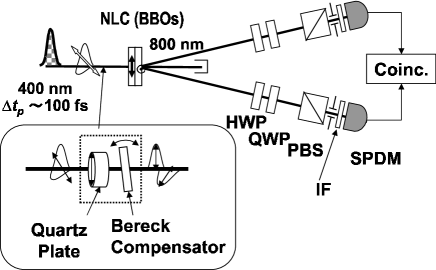
Figure 1: Schematic of the entangled photon pair generation by spontaneous parametric down conversion. Cascade of the nonlinear crystals (NLC) generate the photon pairs. Group velocity dispersion and birefringence in the NLCs are pre-compensated with quartz plates and a Bereck compensator. Two-photon states are analyzed with half wave plates (HWP), quarter wave plates (QWP), and polarization beam splitters (PBS). Interference filters (IF) are placed before the single photon counting modules (SPCM).

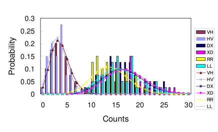
Figure 2: Distribution of the counts obtained in one second on the vectors $|VH\rangle,|HV\rangle,|XD\rangle,|DX\rangle,|RR\rangle,$ and $|LL\rangle$. Bars present the histograms of the measured numbers, and lines show the Poisson distribution with the mean values estimated from the experiment. Measurement time was 40 seconds for each vectors.

In the following, we compare four testing methods on experimental data with the fixed total time $t$. The testing method employ the different time allocations $\{t_{HH},t_{VV},t_{DD},t_{XX},t_{RL},t_{LR},t_{HV},t_{VH},t_{DX},t_{XD},t_{RR},t_{LL}\}$ between the measurement vectors:

(i) Modified visibility method:

$\lambda$ is unknown. The coincidence and the anti-coincidence are measured with the equal time allocation;

$$t_{HH}=t_{VV}=t_{DD}=t_{XX}=t_{RL}=t_{LR}$$

$$=t_{HV}=t_{VH}=t_{DX}=t_{XD}=t_{RR}=t_{LL}=\frac{t}{12}.$$ (30)

(ii) Design I:

$\lambda$ is unknown. The counts on coincidence and anti-coincidence are measured with the optimal time allocation at the target threshold $F_{0}\leq 0.899519$;

$$t_{HH} =t_{VV}=t_{DD}=t_{XX}=t_{RL}=t_{LR}=\frac{t_{1}}{6}$$

$$t_{HV} =t_{VH}=t_{DX}=t_{XD}=t_{RR}=t_{LL}=\frac{t_{2}}{6},$$ (31)

where

$$t_{1} =\frac{t\sqrt{2-2F_{0}}}{\sqrt{2F_{0}+1}+\sqrt{2-2F_{0}}}$$

$$t_{2} =\frac{t\sqrt{2F_{0}+1}}{\sqrt{2F_{0}+1}+\sqrt{2-2F_{0}}}.$$ (32)

(iii) Design II:

$\lambda$ is known. Only the counts on anti-coincidence are measured with the equal time allocation at the target threshold $F_{0}\geq 1/4$;

$$t_{HV} =t_{VH}=t_{DX}=t_{XD}=t_{RR}=t_{LL}=\frac{t}{6}.$$ (33)

(iv) Design III:

$\lambda$ is known. Only the counts on anti-coincidence are measured. The time allocation is given by the two-stage method:

$$t_{HV}=t_{VH}=t_{DX}=t_{XD}=t_{RR}=t_{LL}=\frac{t_{f}}{6}$$ (34)

in the first stage, and

$$\tilde{t}_{xy}=\frac{m_{xy}}{\sum_{(x,y)\in B}\sqrt{m_{xy}}}(t-t_{f})$$ (35)

in the second stage. The observed count $m_{xy}$ in the first stage determines the time allocation in the second stage.

We have compared the p-values at the fixed threshold $F_{0}=7/8=0.875$ with the total measurement time $t=240$ seconds. As shown in section II.2, the p-value measures the minimum risk probability to reject the hypothesis $H_{0}$, i.e., the probability to make an erroneous decision to accept insufficiently entangled states with the fidelity less than the threshold. The results of the experiment and the analysis of obtained data are described in the following.

In the method (i), we measured the counts on each vectors for $20$ seconds. We obtained $n_{1}=9686$ and $n_{2}=868$ in the experiment, which yielded the p-value $0.343$.

In the method (ii), the optimal time allocation was calculated with (32) to be $t_{1}=55.6$ seconds and $t_{2}=184.4$ seconds. However, since the time allocation should be the integral multiple of second in our experiment, we used the time allocation $t_{1}=54$ and $t_{2}=186$. That is, we measure the count on each coincidence vectors for $9$ seconds and on each anti-coincidence vectors for $31$ seconds. We obtained $n_{1}=7239$ and $n_{2}=2188$ in the experiment, which yielded the p-value $0.0715$.

In the method (iii), we measured the count on each anti-coincidence vectors for $40$ seconds. We used $\lambda=290$ estimated from another experiment. We obtained $n=2808$ in the experiment, which yielded the p-value $0.0438$.

In the method (iv), the calculation is rather complicated. Similarly to (iii), $\lambda$ was estimated to be $290$ from another experiment. In the first stage, we measured the count on each anti-coincidence vectors for $t_{f}/6=1$ second. We obtained the counts $6,3,13,20,11$, and $23$ on the vectors $|HV\rangle$, $|VH\rangle$, $|DX\rangle$, $|XD\rangle$, $|RR\rangle$, and $|LL\rangle$, respectively. We made the time allocation of remaining 234 seconds for the second stage according to (35), and obtained $t_{HV}=28.14$, $t_{VH}=19.90$, $t_{DX}=41.42$, $t_{XD}=51.37$, $t_{RR}=38.10$, and $t_{LL}=55.09$. Since the time allocation should be the integral multiple of second in our experiment, we used the time allocation $\{t_{HV},t_{VH},t_{DX},t_{XD},t_{RR},t_{LL}\}=\{28,20,42,51,38,55\}$. We obtained the counts on anti-coincidence $n_{HV}=99,n_{VH}=66,n_{DX}=703,n_{XD}=863,n_{RR}=531$, and $n_{LL}=853$. Applying the counts and the time allocation to the formula (28), we obtained the p-values to be 0.0310.

The p-values obtained in the four methods are summarized in the table. We also calculated the p-values at different values of the threshold $F_{0}$ as shown in Fig. 3. We fixed time allocation for design I at $t_{1}=54$ s and $t_{2}=186$ s. As clearly seen, the optimal time allocation between the coincidence vectors measurement and the anti-coincidence vectors measurement reduces the risk of a wrong decision on the fidelity (the p-value) in analyzing the experimental data. The counts on the anti-coincidence vectors is much more sensitive to the degradation of the entanglement. This matches our intuition that the deviation from zero provides a more efficient measure than that from the maximum does. The comparison between (iii) and (iv) shows that the risk can be reduced further by the time allocation between the anti-coincidence vectors, as shown in Fig. 3. The optimal (Neyman) allocation implies that the measurement time should be allocated preferably to the vectors that yield more counts. Under the present experimental conditions, the optimal allocation reduces the risk probability to about 75 %. The improvement should increased as the fidelity. However, the experiment showed almost no gain when the visibility was larger than 0.95. In such high visibility, errors from the maximally entangled state are covered by dark counts, which are independent of the setting of the measurement apparatus.

	(i)	(ii)	(iii)	(iv)
p-value at $0.875$	0.343	0.0715	0.0438	0.0310

Figure 3: Calculated p-value as a function of the threshold. Dash-dot: (i)the modified visibility, dash: (ii)design I, dot: (iii)design II, solid: (iv) design III.

IX Conclusion

We have applied the formulation of the hypothesis testing scheme and the design of experiment for the hypothesis testing of entanglement to the two-photon state generated by SPDC. Using this scheme, we have handled the fluctuation in the experimental data properly. It has been experimentally demonstrated that the optimal time allocation improves the test in the terms of p-values: the measurement time should be allocated preferably to the anti-coincidence vectors in order to reduce the minimum risk probability. This design is particularly useful for the experimental test, because the optimal time allocation depends only on the threshold of the test. We don’t need any further information of the probability distribution and the tested state. We have also experimentally demonstrated that the test can be further improved by optimizing time allocation among the anti-coincidence vectors by using the two-stage method, when the error from the maximally entangled state is anisotropic.

References

- (1) A. Aspect, P. Grangier, and G. Roger, Phys. Rev. Lett., 49, 91 (1982).
- (2) J. S. Bell. Speakable and Unspeakable in Quantum Mechanics: Collected Papers on Quantum Philosophy, Cambridge University Press, Cambridge, 1993.
- (3) P. W. Shor, SIAM J. Comp. 26, 1484 (1997).
- (4) P.W. Shor and J. Preskill, Phys. Rev. Lett., 85, 441 (2000).
- (5) C. H. Bennett and G. Brassard, Proc. Int. Conf. Comput. Syst. Signal Process., Bangalore, 1984, pp. 175-179.
- (6) H.-J. Briegel, W. Dur, J.I. Cirac, and P. Zoller, Phys. Rev. Lett., 81, 5932 (1998).
- (7) C.H. Bennett, G. Brassard, C. Crépeau, R. Jozsa, A. Peres, and W. K. Wootters, Phys. Rev. Lett. 70, 1895 (1993).
- (8) C. W. Helstrom, Quantum detection and estimation theory, Academic Press (1976).
- (9) A. S. Holevo, Probabilistic and statistical aspects of quantum theory, North-Holland Publishing (1982).
- (10) M. Hayashi, Asymptotic Theory Of Quantum Statistical Inference: Selected Papers, World Scientific (2005).
- (11) A. G. White, D. F. V. James, P. H. Eberhard, and P. G. Kwiat, Phys. Rev. Lett., 83, 3103 (1999).
- (12) K. Usami, Y. Nambu, Y. Tsuda, K. Matsumoto, and K. Nakamura, “Accuracy of quantum-state estimation utilizing Akaike’s information criterion,” Phys. Rev. A, 68, 022314 (2003).
- (13) M. Barbieri, F. De Martini, G. Di Nepi, P. Mataloni, G. M. D’Ariano, and C. Macchiavello, Phys. Rev. Lett., 91, 227901 (2003).
- (14) Y. Tsuda, K. Matsumoto, and M. Hayashi. “Hypothesis testing for a maximally entangled state,” quant-ph/0504203.
- (15) M. Hayashi, A. Tomita, K. Matsumoto, Statistical analysis on testing of an entangled state based on Poisson distribution framework, quant-ph/0608022.
- (16) P. G. Kwiat, E. Waks, A. G. White, I. Appelbaum, and P.H. Eberhard, Phys. Rev. A, 60, 773(R) (1999).
- (17) Y. Nambu, K. Usami, Y. Tsuda, K. Matsumoto, and K. Nakamura, Phys. Rev. A, 66, 033816 (2002).
- (18) E. L. Lehmann, Testing statistical hypotheses, Second edition. Wiley (1986).
- (19) W. G. Cochran, Sampling Techniques, third edition, John Wiley, (1977).