Dissipative dynamics of circuit-QED in the mesoscopic regime

Abstract

We investigate the behavior of a circuit QED device when the resonator is initially populated with a mesoscopic coherent field. The strong coupling between the cavity and the qubit produces an entangled state involving mesoscopic quasi-pointer states with respect to cavity dissipation. The overlap of the associated field components results in collapse and revivals for the Rabi oscillation. Although qubit relaxation and dephasing do not preserve these states, a simple analytical description of the dissipative dynamics of the circuit QED device including cavity relaxation as well as qubit dissipation is obtained from the Monte-Carlo approach. Explicit predictions for the spontaneous and induced Rabi oscillation signals are derived and sucessfully compared with exact calculations. We show that these interesting effects could be observed with a 10 photon field in forthcoming circuit QED experiments.

I Introduction

Cavity quantum electrodynamics is an ideal playground for the realization of tests of quantum processes, simple quantum information processing and exploration of the quantum/classical boundary. Mesoscopic superpositions made of coherent field components with different classical attribues (phase and amplitude) and their decay as a result of decoherence have been observed in experiments involing circular Rydberg atoms Brune et al. (1996a). Recently, an experimental scheme for cavity QED experiments using Josepshon qubits embedded in a superconducting microstrip planar resonator has been proposed Blais et al. (2004) and realized Wallraff et al. (2004) by the Schoelkopf group at Yale. Relying on conventional lithography and nanofrabrication techniques, these circuit-QED devices open the way to scalable quantum circuits coupling qubits to high-$Q$ cavities acting as quantum buses. Recent experimental progresses on these devices have been dramatic, leading to the experimental demonstration of quantum non-demolition measurements of the qubit state in the dispersive regime Wallraff et al. (2005) and of the resolution of photon number states of the cavity Schuster et al. (2007).

These recent developements provide a strong motivation toward studying the dynamics of circuit QED devices at the quantum/classical boundary. In particular, it is important to analyze their ability to produce mesoscopic Schrődinger cat states involving coherent components with a mesoscopic number of photons. Such states can be produced in the dispersive regime where the off resonant qubit acts as a state dependant transparent dielectrics. In this regime, the interaction between a coherent field and a qubit, initially prepared in a superposition of states naturally leads to a quantum superposition of phase shifts.

A much faster way to produce entangled qubit + cavity states is to use a resonant qubit + cavity interaction. In the mesoscopic regime, photon graininess rapidely casts the initially coherent cavity field into a superposition of two components with different phases Gea-Banaloche (1991). This phase splitting is a mesoscopic effect that disappears in the classical limit of a very large field, which is then left unaffected by the atoms. Thus, in the mesoscopic limit, the cavity field acts as a which-path detector for the atomic states. The overlap of field components of the qubit + cavity state is responsible for the collapse and revivals of Rabi oscillations which can be either spontaneous or induced by an echo sequence. This resonant phase splitting effect has been evidenced in Rydberg atom experiments for fields containing up to a few tens of photons Auffeves et al. (2003). Its coherence has been checked using an echo technique borrowed from NMR Meunier et al. (2005), following a proposal by Morigi et al Morigi et al. (2002).

In the presence of dissipation, the entangled qubit + cavity state is subject to decoherence which leads to a damping of the spontaneous and induced Rabi oscillation revivals. In a previous work Meunier et al. (2006), we have developped a simple analytical model that describes the behaviour of $N$ identical non dissipative qubits resonantly and symmetrically coupled to a high-$Q$ cavity. Considering cavity relaxation as the source for decoherence, this model is perfectly well suited for describing Rydberg atom experiments. But this is not sufficient for circuit QED since it does not take into account qubit relaxation and dephasing.

The purpose of the present paper is to present a simple analytical model that takes into account qubit relaxation and dephasing for a single qubit in a cavity thus generalizing results previously obtained by Gea-Banacloche Gea-Banacloche (1993) and ourselves Meunier et al. (2006). Using the physical insight provided by the stochastic wave function approach Dalibard et al. (1992), an analytic description for the decoherence of the mesoscopic qubit + cavity state is derived. Our derivation also sheds light on the range of validity of our previous analysis: whenever the internal interactions within a mesoscopic device tend to produce pointer states with respect to the dominant coupling to the environment, its evolution can described in term of these pointer states and decoherence functionals reflecting the cumulative imprints they left in the environment. In circuit-QED devices, this simple image is broken by qubit dissipative processes but a careful analysis of the dynamics enables us to obtain simple analytical results for the spontaneous and induced Rabi oscillation signals. In principle our analysis can be also used to discuss field tomography and can also be extended to the case of several qubits.

This paper is organized as follows. In Sec. II, the basic model for cavity-QED is presented, its dynamics in both resonant and dispersive regimes are briefly recalled. In Sec. III, circuit-QED devices are presented and dissipation sources are discussed. In Sec. IV, the dissipative dynamics of a one qubit circuit-QED device is studied within the stochastic wave function framework. For completeness, analytical results are derived both for the resonant and dispersive regimes, recovering in the latter case results from the Yale group Gambetta et al. (2006). Section V presents numerical results obtained from quantum Monte-Carlo simulations in the resonant regime. These are used to discuss the validity of our analytical model and to derive experimentally accessible windows for the observation of mesoscopic qubit + cavity states in forthcoming circuit-QED devices. In the conclusion, we comment on the inclusion of other dissipative effects which may be relevant in the study of other cavity QED superconducting circuits Buisson and Hekking (2001).

II Cavity QED

II.1 The model

The effective Hamiltonian describing the cavity QED systems is the Jaynes-Cummings Hamiltonian Jaynes and Cummings (1963) involving the coupling of an harmonic mode to a two level system (the qubit):

$$\hbar^{-1}H_{\mathrm{JC}}=\omega_{0}\,a^{\dagger}a+\frac{\omega_{\mathrm{qb}}}{2}\,\sigma^{z}+\frac{g}{2}(a^{\dagger}\sigma^{-}+a\,\sigma^{+})\,.$$ (1)

In the strong coupling regime, the coupling energy $g$ is assumed to be much larger than all energy scales characterizing dissipative processes in the system, i.e. the cavity relaxation rate $\kappa$ and the atomic relaxation and dephasing rates. Neglecting damping, the Jaynes-Cummings Hamiltonian can be exactly diagonalized since the Hilbert space decomposes into two dimensional multiplets generated by the states $|e,n\rangle=|+\rangle\otimes|n\rangle$ and $|g,n+1\rangle=|-\rangle\otimes|n\rangle$. As a function of the qubit / cavity detuning $\Delta=\omega_{\mathrm{qb}}-\omega_{0}$, the cavity + qubit system has two different regimes.

II.2 The dispersive regime

The dispersive regime is reached when the cavity and the qubit are out of resonance. For an initally empty cavity, it is obtained for $|\Delta|\gg g$. In this regime, the eigenstate are very close to the ones of the uncoupled cavity + qubit states. Performing a second order expansion in $g/\Delta$ leads to

$$\hbar^{-1}H_{\mathrm{disp}}=(\omega_{0}+\chi\sigma^{z})\,a^{\dagger}a+\frac{1}{2}(\omega_{\mathrm{qb}}+\chi)\,\sigma^{z}\,.$$ (2)

where $\chi=g^{2}/4\Delta$ represent the ac-Stark shift per photon. In the presence of a mesoscopic coherent state with average photon number $\bar{n}$, the cavity + qubit coupling is enhanced by the coherent field. Off diagonal terms in the Jaynes Cummings multiplet are small compared to diagonal ones when $|\Delta|\gg g\sqrt{\bar{n}}$.

In the dispersive regime, qubit flips can only occur because of qubit relaxation or external driving of the system. With respect to the cavity mode, the qubit behaves as a transparent medium with a state-dependent refraction index. In Rydberg atom experiments, this regime has been used to produce Schrődinger cat states Brune et al. (1996a), to perform QND measurement of the photon number Gleyzes et al. (2007) and a measurement of the Wigner function of the field Bertet et al. (2002). In circuit QED devices, the cavity has been used to performed a QND measurement of the qubit state Wallraff et al. (2005). More recently, the strong coupling dispersive regime where a single photon drastically alters the qubit absorbtion spectrum has been has been studied theoretically Gambetta et al. (2006) and demonstrated experimentally Schuster et al. (2007).

II.3 The resonant regime

The resonant regime is obtained when $\Delta=0$. In this case, the Jaynes-Cummings eigenstates are symmetric and antisymmetric combinations of the form $(|e,n\rangle\pm|g,n+1\rangle)/\sqrt{2}$ separared by an energy $g$ (vacuum Rabi splitting). This leads to vacuum Rabi oscillations between states $|e,0\rangle$ and $|g,1\rangle$ which have been observed Brune et al. (1996) and used to transfer the qubit state in the cavity Maitre et al. (1997). In the mesoscopic regime $\bar{n}\gg 1$, the resonant interaction leads to an entangled atom-field state with two quasi-coherent field components with different classical phases Gea-Banaloche (1991). The approximate solution by Gea-Banacloche precisely provides explicit expression for these states and provides the basic framework for discussing the complete dissipative dynamics of circuit QED devices.

It has proven very convenient to describe the dynamics using an effective Hamiltonian approach that involves effective spin operators acting within the Jaynes-Cummings multiplet Klimov and Chumakov (1995); Meunier et al. (2006). Within the framework of this mesoscopic approximation ($\bar{n}\gg 1$ and $t\ll\bar{n}/g$), the evolution of the cQED system can be computed exactly. Under the Jaynes-Cummings Hamiltonian, in the mesoscopic regime, the states

$$|\Psi_{\pm}^{X}(\theta)\rangle=e^{-\frac{\bar{n}}{2}}\sum_{p=0}^{\infty}\frac{\bar{n}^{p/2}}{\sqrt{p!}}\,e^{\mp i\theta\sqrt{p+1}/2}\,|X_{\pm}^{(p)}\rangle$$ (3)

where $|X^{(p)}_{\pm}\rangle=(|e,p\rangle\pm|g,p+1\rangle)/\sqrt{2}$ remain of the same form with a time dependent angle $\dot{\theta}(t)=g$. In the mesoscopic approximation, $|\Psi_{\pm}^{X}(\theta)\rangle$ can be approximated by a factorized state of the form Meunier et al. (2006):

$$|\Psi_{\pm}^{X}(\theta)\rangle\simeq e^{\mp i\theta\sqrt{\bar{n}}/2}\,|D_{\pm}(\theta)\rangle\otimes|\psi_{\pm}(\theta)\rangle$$ (4)

where the atomic polarization is given by:

$$|D_{\pm}(\theta)\rangle=\frac{1}{\sqrt{2}}\left(\pm e^{\mp i\theta}|+\rangle+|-\rangle\right)$$ (5)

and the field component is

$$|\psi_{\pm}(\theta)\rangle=e^{\pm i\theta\sqrt{\bar{n}}/2}\,e^{-\bar{n}/2}\sum_{k=0}^{+\infty}\frac{\bar{n}^{k/2}}{\sqrt{k!}}\,e^{\mp i\theta\sqrt{k}/2}\,|k\rangle\,.$$ (6)

The field state $|\psi_{\pm}(\theta)\rangle$ is proportional to a quasi coherent state whose parameter is roughly equal to $\sqrt{\bar{n}}\,e^{\mp i\theta/4\sqrt{\bar{n}}}$. At fixed $\bar{n}$, the phase, in Fresnel plane, associated with the generalized Gea-Banacloche state $|\Psi^{X}_{m}(\theta)\rangle$ is $\phi_{m,\theta}=-m\theta/2\sqrt{\bar{n}}$. The atomic polarization evolves in the equatorial plane of the Bloch spere, its phase being perfectly correlated to the electromagnetic phase.

The states $|\psi_{\pm}(\theta)\rangle$ act as a path detector for the atomic polarizations $|D_{\pm}(\theta)\rangle$ and this explains the pattern of collapses and revivals of Rabi oscillations. When $t\ll g^{-1}$, the field components $|\psi_{\pm}(gt)\rangle$ still overlap and therefore, Rabi oscillations arising from interference between the $|D_{+}\rangle$ and $|D_{-}\rangle$ are observed. Once $gt\gtrsim 2\pi$, the field components do not overlap and Rabi oscillations disappear. Only when $gt/2\sqrt{\bar{n}}$ is a multiple of $2\pi$, the two states overlap again. The information about the qubit state stored by into the cavity is erased, thus leading to a revival of Rabi oscillations. Henceforth, collapses and revivals of Rabi oscillations in the mesoscopic regime are a direct illustration of the complementarity principle.

When $gt/2\sqrt{\bar{n}}=\pi$, the qubit polarizations will coincide. Then, the atom + cavity state disentangles and the resulting cavity state is a mesoscopic Schrődinger cat states involving two quasi-coherent components with opposite phases. This occurs much faster than in the dispersive regime $|\Delta|\gg g\sqrt{\bar{n}}$ where such a Schrődinger cat state would be generated in $\pi|\Delta|/g^{2}\gg 2\pi\sqrt{\bar{n}}/g$.

III Circuit QED devices

Recent experiments performed at Yale involve the coupling of a superconducting Josephson qubit and a superconducting microstrip resonator with high quality factor Wallraff et al. (2004). We will first present these devices and recall how they can be described by the Jaynes-Cummings Hamiltonian. Dissipation sources will then be discussed.

III.1 The cavity: a superconducting microstrip resonator

The resonator is 1D a transmission line made by photolithography whose lowest mode lies within the 1-10 GHz frequency range and whose quality factors can be as high as $10^{6}$ Frunzio et al. (2005). Besides this, the electromagnetic field associated with their eigenmodes is confined within a relatively small volume, thus leading to high electric fields between the center and ground planes (typically $0.2$ V/m). Such a resonator is usually characterized by a wave velocity $v$, a real impedance $R$ ans its length $L$.

The finite length superconducting resonator has many stationary modes up to a certain high frequency cutoff but in the present situation, only the coupling to the lowest energy mode The voltage difference between the inner and outer electrodes at point $x$ is then expressed in terms of the mode creation and destruction operators:

$$V(x)=V_{0}\,(a+a^{\dagger})\,\sin{\left(\frac{\pi x}{L}\right)}$$ (7)

where $V_{0}$ denotes the maximum voltage felt by the qubit.

III.2 The artificial atom: a Josephson qubit

Within the resonator lies a superconducting Josephson charge qubit (initially a Cooper pair box) coupled to the cavity electric field. It consists in a small superconducting island connected to a superconducting reservoir through a very thin insulating barrier. When the temperature $k_{B}T$ and the the Coulomb charging energy of the island $E_{c}$ are smaller than the superconducting gap, the qubit degrees of freedom are encoded by the charge state of the superconducting island. This device can be characterized by the Josephson amplitude $E_{J}$ and the Coulomb energy $E_{c}$. Control parameters are the voltage potential $V_{g}$ imposed to the superconducting island and the Josephson amplitude which can be tuned using a SQUID instead of a single Josephson junction Makhlin et al. (2001): $E_{J}=\mathcal{E}_{J}\,\cos{(2\pi\Phi_{J}/\Phi_{0})}$ where $\Phi_{0}=2e/h$ denotes the flux quantum and $\Phi_{J}$ the magnetic flux through the SQUID.

In the charge regime $E_{c}\ll E_{J}$ and for gate charge $n_{g}=C_{g}V_{g}/2e$ restricted to a unit charge interval $0\leq n_{g}\leq 1$, the system effectively behaves like a two level system (TLS) involving two adjacent charge states of the island. In this charge basis, its effective Hamiltonian is given by:

$$H_{\mathrm{qb}}=-\frac{B_{z}}{2}\,\sigma^{x}-\frac{B_{x}}{2}\,\sigma^{z}$$ (8)

where $B_{z}=4E_{c}(1-2n_{g})$ and $B_{x}=E_{J}$.

III.3 The qubit/cavity coupling

The electromagnetic mode of the 1D cavity naturally couples to the qubit charge through capacitance between the resonator inner and outer electrodes. The coupling $g$ energy is limited by the dipolar energy of the qubit within the resonator: $g/\omega_{0}\lesssim\lambda_{\mathrm{c}}\sqrt{R/R_{q}}$ where $\lambda_{\mathrm{c}}$ is a capacitance ratio and $R_{q}=h/e^{2}$ is the quantum of resistance. Classical electrodynamics shows that $R$ is of the order of $2R_{q}\alpha\Lambda/\epsilon_{r}$ where $\alpha$ is the fine structure constant, $\epsilon_{r}$ is the relative permittivity and $\Lambda$ a geometric factor, usually logarithmic in the microstrip aspect ratios. Within the 1 to 10 GHz frequency range, values of $g/2\pi$ range from 11 to 105 MHz (see table 1) the latter value being obtained using the ”transmon” Koch et al. (2007). Assuming that the two level description of the qubit is valid, the coupling Hamiltonian between the qubit and the cavity is given by:

$$H_{\mathrm{int}}=\hbar g\,(a+a^{\dagger})(1-2n_{g}-\sigma^{x})\,.$$ (9)

The coupling being small compared to the resonator and qubit eigenfrequencies, the rotating wave approximation is valid and close to the charge degeneracy point $n_{g}\simeq 1/2$, eq. (9) reduces to the Jaynes-Cummings Hamiltonian (1).

III.4 Measurement protocols

In these experiments, the Josephson qubit cannot be measured directly. This circuit-QED system is probed through the resonator which is then connected to external ports at its ends. A network analyzer is used to analyzed the phase and amplitude of a classical electromagnetic wave transmitted through the device. This method has been used to perform a non-destrictive measurement of the qubit state using a dispersive measurement technique Wallraff et al. (2005). Thus, the relaxation time scale of the resonator $\kappa^{-1}$ sets a lower bound on the measurement time. Probing the state of the qubit thus requires that $\kappa\gtrsim\gamma_{2}$ where $\gamma_{2}=\gamma_{1}+\gamma_{\varphi}/2$. Although cavities with quality factors of the order of $10^{6}$ have been manufactured Frunzio et al. (2005), devices used in experiments have a lower $Q$ in order to satisfy the fast measurement constraint.

In order to avoid this limitation, one has to rely on an alternative method for measuring the qubit state. Recently, a new detection scheme based on the dynamical bifurcation of Josephson junction has been realized and provides a high contrast, low backaction, dissipationless and fast measurement of the qubit state Siddiqi et al. (2005). Thus, rapid improvement of Josepshon circuit technology suggests that alternative methods of detection might become available in the near future.

In the present paper, we focus on the evolution of the qubit + cavity system prior to measurement. In particular, our main objective is to describe the dynamics of the circuit QED system at resonance in the mesoscopic regime and shed light on the main physical effects independantly from the measurement protocol. Therefore, for the sake of simplicity, we will not attempt modeling the subsequent measurement process.

III.5 Dissipation mechanisms

III.5.1 Qubit relaxation and dephasing

Qubit dissipation and decoherence arise from their coupling to environmental degrees of freedom either extrinsinc (measurement circuit) or intrinsic (structural defects inside the material). Relaxation involves energy exchange between the qubit and its environment and, as such, is generically sensitive to the low frequency part of the environmental spectrum. Relaxation also leads to decoherence defined as the decay of off diagonal matrix element in the qubit’s eigenbasis.

But dephasing can also occur without energy exchange (pure dephasing). Early circuit-QED experiments used a Cooper pair box. The coherence properties of these devices are limited by pure dephasing induced by low frequency noise. It arises from fluctuating charges in the insulating amorphous $\mathrm{Al}_{2}\mathrm{O}_{3}$ used to make the Josephson junctions Astafiev et al. (2004). It is known that the effect of this low frequency noise cannot be described within a Markovian framework Makhlin and Shnirman (2003). A possible escape to this problem is to operate the qubit at special point where sensitivity to voltage fluctuations is at second order instead of first order Vion et al. (2002). At this working point, treating the effect of low frequency noise requires going beyond the Markovian approximation Makhlin and Shnirman (2004); Ithier et al. (2005). Fortunately recent circuit QED experiments use another type of qubit, called the ”transmon” which has very low sensitivity to voltage fluctuations (sweet spot everywhere), can be operated as a two level system and the low frequency noise Koch et al. (2007). Therefore, having in mind future experiments performed with transmons, qubit relaxation and dephasing will be treated within the Markovian approximation in the present paper.

Under this hypothesis, the evolution of the qubit + cavity system reduced density operator is described by a master equation of the form:

$$\frac{d\rho}{dt}=-\frac{i}{\hbar}\,[H,\rho]+\sum\mathcal{L}_{j}(\rho)$$ (10)

where $H$ denotes the Jaynes-Cummings Hamiltonian (1) and $\mathcal{L}_{j}(\rho)$ are the Lindbladian superoperators associated with each markovian dissipation channel.

The relaxation Lindbladian operator is given by:

$$\mathcal{L}_{r}(\rho)=\gamma_{1}\,\left(\sigma^{-}\ldotp\rho\ldotp\sigma^{+}-\frac{1}{2}\,\left\{\frac{1+\sigma^{z}}{2},\rho\right\}\right)\,.$$ (11)

where $\gamma_{1}$ represents the relaxation rate of the isolated qubit. Markovian pure dephasing corresponds to the difusion of the relative phase between states $|\pm\rangle$. The pure dephasing Lindbladian operator is then given by:

$$\mathcal{L}_{r}(\rho)=\frac{\gamma_{\varphi}}{2}\left(\sigma^{z}\ldotp\rho\ldotp\sigma^{z}-\rho\right)\,.$$ (12)

where $\gamma_{\varphi}$ is the pure dephasing rate of the qubit defined as the decaying rate of the $\langle+|\rho(t)|-\rangle$ off diagonal matrix element for a standalone qubit.

III.5.2 Resonator relaxation

In the case of the circuit-QED devices, relaxation mainly comes from capacitives losses at the ends of the resonator. The temperature dependance can be explained by considering that the inverse quality factor $Q^{-1}$ is a sum of two contributions. The first contribution represents thermal breaking of Cooper-pairs in the superconductor and it scales as $\exp{(T_{c}/T)}$. The other contribution has a much weaker temperature dependance and is probably associated with intrinsic dissipation mechanisms such as dielectric losses or magnetic vortices Frunzio et al. (2005). This term is responsible for the low temperature value of quality factor. Note that the current limitation in the quality factor of microwave cavities used in Rydberg atom experiments comes from diffraction losses, surface rugosity and residual resistance of the superconducting mirrors coming from defects, impurities and magnetic vortices Kuhr et al. (2006).

The corresponding Lindbladian is then:

$$\mathcal{L}_{c}(\rho)=\kappa\,\left(a\ldotp\rho\ldotp a^{\dagger}-\frac{1}{2}(a^{\dagger}a\ldotp\rho+\rho\ldotp a^{\dagger}a)\right)\,.$$ (13)

where $\kappa$ denotes the total relaxation rate of the oscillator.

IV Dissipative dynamics

IV.1 The stochastic wave function method

In principle, eq. (10) can be solved numerically in order to obtain the quantum dynamics. However, an analytical ansatz for the reduced density matrix can be found within the mesoscopic approximation using the the quantum jump approach Dalibard et al. (1992) to the dissipative dynamics of the atoms + cavity system. As we shall see extensively in this paper, it provides a deep and useful insight into the full dissipative dynamics of the cQED system and will enable use to find simple analytical results for the Rabi oscillation signals.

The quantum jump method provides a solution to the master equation (10) by assuming that the environment of the system is continuously monitored so that any emission or absorption of quanta by the system can be assigned a precise, although stochastic date. Each time such an event occurs, the system undergoes a quantum jump:

$$|\psi(t^{+})\rangle=\frac{L_{j}\,|\psi(t)\rangle}{\sqrt{\langle L_{j}^{\dagger}L_{j}\rangle_{|\psi(t^{-})\rangle}}}\,.$$ (14)

The probability rates at a given time $t$ for the various quantum jumps are directly obtained as averages $\langle L_{j}^{\dagger}L_{j}\rangle_{|\psi(t^{-})\rangle}$ where the $L_{j}$ denote the quantum jump operator of type $j$. Here, the quantuum jump operators associated to pure dephasing, qubit relaxation and cavity relaxation are respectively equal to: $L_{\varphi}=\sqrt{\gamma_{\varphi}/2}\,i\sigma^{z}$ corresponding to a $\pi$ rotation around the $z$ axis, $L_{R}=\sqrt{\gamma_{1}}\,\sigma^{-}$ and $L_{\mathrm{c}}=\sqrt{\kappa}\,a$.

Between these jumps, the evolution is described by an effective Hamiltonian that describes both its intrinsic dynamics and the acquisition of information arising from the fact that no quanta has been detected:

$$H_{\mathrm{eff}}=H-\frac{i\hbar}{2}\sum_{j}\,L^{\dagger}_{j}L_{j}\,.$$ (15)

The reduced density matrix is then recovered by averaging over the set of stochastic trajectories associated with a large set of quantum jumps sequences. The weight of a given trajectory can be directly related to the dates and types of the various quantum jumps. The corresponding Linbladian is then given by:

$$\mathcal{L}_{j}(\rho)=L_{j}\ldotp\rho\ldotp L_{j}^{\dagger}-\frac{1}{2}\{L_{j}^{\dagger}L_{j},\rho\}\,.$$ (16)

This method proves to be very convenient numerically since the number of variables involved is of the order of the dimension $d$ of the system’s Hilbert space whereas it scales as $d^{2}$ in the master equation approach.

IV.2 Pointer states dynamics

A general stochastic dynamics tends to produce arbitrary mixtures of states. However, it takes a very simple form for states that are preserved (up to a phase) between and during quantum jumps. These so called pointer states entangle minimally with the system’s environment. In some cases, they provide a basis of the system’s Hilbert space, thus leading to a simple description of the stochastic dynamics which we call a pointer state dynamics.

Since coherent states are pointer states with respect to cavity losses, such a description is directly relevant for the describing the effect of cavity relaxation on cavity QED systems in both dispersive and resonant regime.

IV.2.1 General results

We assume that each eigenvalue of the quantum jump operator $L$ is non degenerate and choose a fixed section $\lambda\mapsto|\lambda\rangle$ ($L|\lambda\rangle=\lambda\,|\lambda\rangle$) of the corresponding vector bundle over $L$’s spectrum. Pointer states $|\lambda\rangle$ remain pointer states in the evolution between quantum jumps as soon as $[L,H]=h(L)$ and $[L,L^{\dagger}L]=f(L)$ (sufficient condition). In this case, evolution beween quantum jumps of $|\lambda\rangle$ produces a single quantum trajectory $t\mapsto e^{i\theta(\lambda,t)}\,|\lambda(t)\rangle$ where:

$$\frac{d\lambda(t)}{dt}=-\frac{i}{\hbar}\,h(\lambda(t))-\frac{\gamma}{2}\,f(\lambda(t))$$ (17)

with initial condition $\lambda(0)=\lambda$. The phase $\theta(\lambda,t)$ contains an Hamiltonian and a Berry phase contribution:

$$\theta_{t}[\lambda] = -\frac{1}{\hbar}\int_{0}^{t}\langle\lambda(\tau)|H|\lambda(\tau)\rangle\,d\tau$$ (18)

$$+ \int_{0}^{t}\Im{(\langle\dot{\lambda_{\tau}}|\lambda(\tau)\rangle)}\,d\tau$$ (19)

Then, starting from a single pointer state $|\lambda\rangle$, the stochastic dynamics taking into account all possible sequences of quantum jumps occuring at times $0\leq t_{1}\leq\ldots\leq t_{p}\leq t$ produces a single trajectory $t\mapsto\lambda(t)$ but encodes the sequence of quantum jumps in a $(t_{1},\ldots,t_{p})$ dependent phase. The resulting state at time $t$ is of the form $e^{i\theta(t_{1},\ldots,t_{p})}|\lambda(t)\rangle$ and therefore, any initial state which is linear combination of pointer states will experience decoherence because of the averaging of these random phases.

Summing over all quantum jumps sequences leads to the system’s reduced density operator obtained from an initial state $\sum_{\lambda}c_{\lambda}\,|\lambda\rangle$:

$$\rho(t)=\sum_{(\lambda_{+},\lambda_{-})}c_{\lambda_{+}}\,c_{\lambda_{-}}^{*}\,\mathcal{F}_{t}[\lambda_{+},\lambda_{-}]e^{i(\theta_{t}[\lambda_{+}]-\theta_{t}[\lambda_{-}])}|\lambda_{+}(t)\rangle\langle\lambda_{-}(t)|$$ (20)

where the decoherence functional is given by:

$$\mathcal{F}_{t}[\lambda_{+},\lambda_{-}]=e^{-\frac{\gamma}{2}\int_{0}^{t}|\lambda_{+}-\lambda_{-}|^{2}(\tau)\,d\tau}e^{i\gamma\int_{0}^{t}\Im{(\lambda_{+}\lambda_{-}^{*})(\tau))}\,d\tau}\,.$$ (21)

As expected, this expression coincides with the accumulated decoherence of a pair of coherent states driven along trajectories $t\mapsto\lambda_{\pm}(t)$.

IV.2.2 Application to cQED systems

In the dispersive regime of cQED, the effective dissipative dynamics is described by the effective Hamiltonian (2). In the strong coupling regime $g\ll\kappa$, the effective quantum jump operator associated with cavity losses can still be approximated by $L=\sqrt{\kappa}\,a$. Therefore, in this scheme, the pointer states with respect to cavity losses are states of the form $|\pm\rangle\otimes|\alpha\rangle$. Since any state can be expanded as a linear combination of these pointer states, the dispersive regime of cQED realizes the above describes pointer state dynamics. Their respective coherent state parameters evolve according to:

$$\frac{d\alpha_{\pm}}{dt}=-i\omega_{\pm}\,\alpha_{\pm}(t)-\frac{\kappa}{2}\,\alpha_{\pm}(t)-i\epsilon(t)$$ (22)

where $\omega_{\pm}=\omega_{0}\pm\chi$ is the ac-Stark shifted cavity frequency and $\epsilon(t)$ is a driving of the cavity. Starting from an initial state of the form $|\psi_{\mathrm{qb}}\rangle\otimes|\alpha\rangle$ leads to a qubit + cavity reduced density operator of the form (20) involving two pointer states $|+\rangle\otimes|\alpha_{+}(t)\rangle$ and $|-\rangle\otimes|\alpha_{-}(t)\rangle$ where $\alpha_{\pm}(\tau)$ denote solutions of (22) with initial condition $\alpha_{\pm}(0)=\alpha$. The decoherence functional induced by cavity losses and relative to these states is obtained by substituting $\alpha_{\pm}(\tau)$ into (21). As we shall see in more details in section IV.4.2, this is exactly the dynamics solved in Ref. Gambetta et al. (2006) using a different method.

In the case of a qubit resonantly coupled to the cavity, generalized Gea-Banacloche states (3) are approximate pointer states with respect to cavity losses. Let us first consider an initial state of the form $|\psi_{\mathrm{qb}}\rangle\otimes|\alpha\rangle$ where $|\psi_{\mathrm{qb}}\rangle$ is the qubit initial state and where the parameter $\alpha$ of the initial coherent field is taken real. Cavity losses will then produce a qubit + cavity reduced density operator involving two generalized Gea-Banacloche states $|\Psi_{\pm}^{X}(t)\rangle$. The decoherence coefficient in front of the $|\Psi_{+}^{X}(t)\rangle\langle\Psi^{X}_{-}(t)|$ is obtained by substituting $\alpha_{\pm}(t)=\alpha\,e^{\mp igt/4\sqrt{\bar{n}}}$ in (21). Introducing one or several $\pi$-pulses (single echo or bang-bang control) only changes the trajectories of the Gea-Banacloche parameters $\alpha_{\pm}(t)$ in the Fresnel plane but eq. (21) remains valid. To deal with more general initial condition such as $|\psi_{\mathrm{qb}}\rangle\otimes(|\alpha_{1}\rangle+|\alpha_{2}\rangle)$, one just has to decompose the initial state as a sum of rotated generalized Gea-Banacloche states where the $X$ direction is replaced by the directions given by the phases of the coherent states present in the initial condition.

So far, only the effect of cavity losses has been discussed. How do other sources of dissipation affect this picture in the dispersive and the resonant regimes ?

To answer this question, let us first remark that, in the dispersive regime, pointer states with respect to cavity losses are also pointer states with respect to pure dephasing of the qubit. Qubit relaxation sends a pointer state of the form $|+\rangle\otimes|\alpha\rangle$ on a pointer state $|-\rangle\otimes|\alpha\rangle$. Therefore, in the dispersive regime, a pointer state is sent on another pointer state. But the situation is more involved in the resonant or quasi-resonant regimes. However, we shall see that quasi pointer states are sent on linear combinations of quasi pointer states. Thus, the complete stochastic dynamics can still be described in terms of generalized Gea-Banacloche states (3) and for this reason, simple analytical results can still be obtained.

The simpler case of pure dephasing will be considered first and we will then turn to the more complicated case of qubit relaxation. Explicit analytical results for the spontaneous and induced Rabi oscillation signals are given in section IV.5. For the sake of simplicity, the stochastic dynamics will be discussed using the factorized form (4) of generalized Gea-Banacloche states, assuming that their coherence is not broken by the dissipative processes under consideration. This assertion will be justified by a more precise discussion of the dynamics postponed in appendix B.

IV.3 Pure dephasing

IV.3.1 Resonant regime

First of all, let us note that the corresponding quantum jump operator has no effect between quantum jumps. Moreover, the rate of pure dephasing jumps is constant in time, independent of the state and equal to $\gamma_{\varphi}/2$. Next, each quantum jump acts as a $\pi$ rotation around the $z$ axis, exactly like an echo pulse. As such, it sends the atomic polarization $|D_{\pm}(\theta)\rangle$ defined in eq. (5) on $|D_{\mp}(-\theta)\rangle$ not affecting the field component (6). After $p$ jumps occuring at times $0\leq t_{1}\leq\ldots\leq t_{p}\leq t$, an initial state $|D_{m}(0)\rangle\otimes|\psi_{m}(0)\rangle$ has turned into $e^{-im\theta\sqrt{\bar{n}}}\,|D_{m^{\prime}}(\theta_{t})\rangle\otimes|\psi_{m^{\prime}}(\theta_{t})\rangle$ where $m^{\prime}=(-1)^{p}m$ and $\theta_{t}=\theta(t_{1},\ldots,t_{p};t)$ is defined as

$$\theta(t_{1},\ldots,t_{p};t)=g\sum_{j=0}^{p}(-1)^{j}(t_{j+1}-t_{j})$$ (23)

where $t_{0}=0$ and $t_{p+1}=t$.

A typical trajectory $\mathcal{T}$ of the associated phase in Fresnel plane is depicted on figure 1, with slope changing of sign at each quantum jump. The relative phase between the two quasi-coherent field components follows a random trajectory directly related to the integral of a telegraphic noise:

$$(\Delta\phi)(t)=\frac{g}{2\sqrt{\bar{n}}}\,\int_{0}^{t}X(\tau)\,d\tau$$ (24)

where $X(\tau)\in\{-1,1\}$ starts with $X(0)=1$ and jumps each time there is a quantum jump. The probability distribution of waiting times $\tau$ between quantum jumps is exponential $\psi(\tau)=\frac{\gamma_{\varphi}}{2}\,e^{-\gamma_{\varphi}\tau/2}$. The characteristic function of the probability distribution for $(\Delta\phi)(t)$ is nothing but the decoherence coefficient of a qubit in a longitudinal telegraphic noise Paladino et al. (2002). Its behavior depends on the dimensionless parameter $\eta=g/\gamma_{\varphi}\sqrt{\bar{n}}$ which is equal to $2\pi/\overline{N}_{\varphi}$ where $\overline{N}_{\varphi}=2\pi\sqrt{\bar{n}}\gamma_{\varphi}/g$ is the average number of quantum jump events occuring before the date of the first expected Rabi oscillation revival.

Figure 1: Typical trajectory of the phase $\phi$ of the quasi-coherent component state in the Fresnel plane showing two quantum jumps at time $t_{1}$ and $t_{2}$. The effect of a pure dephasing quantum jump is to reverse the direction of motion of the quasi-coherent component in the Fresnel plane. Inset recalls the definition of $\phi$.

For $\eta\gg 1$, only a single event is necessary to spread the phase $(\Delta\phi)(t)$ over $2\pi$. In this regime, the evolution of the cQED system up to the first revival is dominated by quantum trajectories having no pure dephasing quantum jumps. Their total weight is $e^{-\gamma_{\varphi}t/2}\sim 1$. Trajectories with one quantum jump or more have a total weight $1-e^{-\gamma_{\varphi}t/2}\ll 1$ and can therefore be treated perturbatively. For fixed $g$ and $\gamma_{\varphi}$, this ”weak dephasing limit” is realized for $\bar{n}\ll(g/\gamma_{\varphi})^{2}$. In practice, this is the regime of interest for present and forthcoming experiments since $g/\gamma_{\varphi}$ is above 40.

For $\eta\ll 1$, a large number of events are necessary to spread significantly the random relative phase $(\Delta\phi)(t)$. In this case, rapid dephasing of the qubit prevents the observation of an atom + cavity entangled state. As shown in appendix B, the incoherent qubit ends up breaking the coherence of the coherent field, selecting Fock states as pointer states. This is the ”strong dephasing limit” which, as already stressed, can only be reached for very large photon numbers in the strong coupling regime of cQED.

Nevertheless, in the strong dephasing limit, even if the spreading of the field phase takes place over a time scale $2\gamma_{\varphi}\bar{n}/g^{2}\gg\gamma_{\varphi}^{-1}$ the Rabi oscillation signal will be strongly damped in a much shorter time. Indeed for $t\lesssim 2\pi\sqrt{\bar{n}}/g$, although the Fresnel angle of Gea-Banacloche states are weakly dispersed around zero and thus have a rather strong overlap for a typical given quantum trajectory, the classical Rabi oscillation phase $e^{2i\bar{n}\phi_{t}}$ averages to zero over a time scale of the order of $2\gamma_{\varphi}^{-1}$. This means that the qubit dephasing time is anyway the upper limit to the Rabi oscillation visibility in the mesoscopic regime. Nevertheless, for qubits in high quality resonators but rather poor dephasing properties $g/\gamma_{\varphi}\lesssim 5$, the crossover from weak to strong dephasing regimes might be observed by performing a tomography of the field state.

Finally, the result of this analysis is that, in the strong coupling regime of cQED, the main contribution to the Rabi oscillation signal comes from quantum histories without any pure dephasing quantum jump. As far as we are interested by this signal, the effect of qubit dephasing can be accounted for through a supplementary decoherence factor on top of the decoherence factor associated with cavity losses:

$$\mathcal{F}_{+,-}^{(\varphi)}(t)\simeq e^{-\gamma_{\varphi}t/2}\,.$$ (25)

IV.3.2 Dispersive regime

In the dispersive regime, the analysis is much simpler since pointer states with respect to cavity losses are also pointer states with respect to pure dephasing of the qubit. Therefore, starting with an initial state of the form $|\psi_{\mathrm{qb}}\rangle\otimes|\alpha\rangle$, the only effect of pure dephasing is to multiply the decoherence functional associated with cavity losses by:

$$\mathcal{F}_{+-}^{(\varphi)}(t)=e^{-\gamma_{\varphi}t}\,.$$ (26)

IV.4 Qubit relaxation

IV.4.1 Resonant regime

For a standalone qubit, the non hermitian part of the Hamiltonian tends to bring the state of the qubit towards the $|-\rangle$ state, thus reflecting the acquisition of information associated with the absence of relaxation quantum jump. But at resonance, in the presence of a mesoscopic state, the pumping of the qubit by the cavity photons alters the dynamics between quantum jumps. As discussed in appendix A, in the $\gamma_{1}\ll g$ regime, the dynamics is dominated by the strong atoms + cavity coupling. Contrarily to the case of a the dispersive regime where no photon can excite the qubit after relaxation, several relaxation jump can occur. The statistics of relaxation quantum jumps is indeed described by a renewal process with effective waiting time distribution $\psi_{1}(\tau)=(\gamma_{1}/2)e^{-\gamma_{1}\tau/2}$. The effective rate $\gamma_{1}/2$ follows from the localization of generalized Gea-Banacloche states in the equatorial plane of the Bloch sphere.

When the first relaxation quantum jump occurs at time $t_{1}$, the qubit gets projected on the $|-\rangle$ state leaving the cavity in a superposition of quasi-coherent states $|\psi_{\pm}(t_{1})\rangle$. The subsequent Rabi oscillation signal then shows rapid oscillations of frequency $g\sqrt{\bar{n}}$ which correspond to the superposition of the Rabi oscillation signals associated with the evolution of $|-\rangle\otimes|\psi_{\pm}(t_{1})\rangle$. Therefore, the first relaxation jump leaves us with four quasi-coherent components in the Fresnel plane as shown in fig. 2:

$$\sigma^{-}\,|\Psi^{X}_{\pm}(\theta)\rangle=\frac{e^{i\phi_{\pm,\theta}}}{\sqrt{2}}\,\left(|\Psi^{X}_{+}(\theta)\rangle-|\Psi^{X}_{-}(-\theta)\rangle\right)$$ (27)

The Rabi oscillations starting right after the first jump collapse in time $g^{-1}$ due to the splitting of the pairs of counter-rotating quasi components in the Fresnel plane. Revivals then occur when two of them recombine.

Assuming that $gt_{1}/2\sqrt{\bar{n}}<\pi$, the first recombination occurs at time $2t_{1}$ and involves components (b) and (c) on fig. 2). Components (a) and (b) will recombine at time $t_{1}+4\pi\sqrt{\bar{n}}/g$ as well as components (c) and (d). But in these three cases, the rapid oscillations are simply washed out by the averaging over $t_{1}$ as in the pure dephasing case. Only the recombination of components (a) and (d) will not be averaged to zero since it takes place at time $4\pi\sqrt{\bar{n}}/g$, independent of $t_{1}$.

Figure 2: Quasi-coherent components generated after one relaxation jump pictured in the Fresnel plane. Field quasi-coherent states are represented as uncertainty disks at the tip of their classical amplitudes. Components components (b) and (d) move clockwise whereas components (a) and (c) move counterclockwise.

A careful discussion of of all contributions is presented in appendix B. It shows that keeping only the first term in the r.h.s. of (27) corresponds to retaining only trajectories for rapid oscillations survive the averaging over dates of relaxation jumps. Therefore, we are brought back to the case of a single pair of trajectories within the Fresnel plane. But with each relaxation jump comes not only a pure phase as in eq. (38) of Meunier et al. (2006) but a coefficient $e^{-i\phi_{m,\theta}}/\sqrt{2}$. Following Meunier et al. (2006), these coefficients can be resummed thus leading to the decoherence coefficient associated with relaxation in front of the coherence $|\Psi_{+}^{X}(t)\rangle\langle\Psi_{-}^{X}(t)|$:

$$\mathcal{F}^{(R)}_{+-}(t)=\exp{\left(\frac{\gamma_{1}}{2}\int(\frac{1}{2}\,e^{i\Delta\phi(\tau)}-1)\,d\tau\right)}$$ (28)

where $(\Delta\phi)(\tau)=g\tau/2\sqrt{\bar{n}}$ denotes the angular separation in the Fresnel plane of the quasi-component components of $|\Psi_{\pm}^{X}(\tau)\rangle$.

As a final comment of this discussion, let us point out that this decoherence coefficient alone is not sufficient to keep track of the complete state of the atoms + cavity system. More precise results could be obtained by perfoming a pertubative expansion in $\gamma_{1}/g$ keeping track of all contributions arising from (27). Cavity losses and dephasing jumps can then be taken into account. The resulting formula are appropriate in the weak relaxation regime but rapidely require numerical evaluation.

IV.4.2 Dispersive regime

Being off resonance, the cavity cannot send back the qubit to the $|+\rangle$ state after a relaxation quantum jump. As stressed before, since the states $|\pm\rangle\otimes|\alpha\rangle$ are pointer states with respect to cavity relaxation, the relaxation dynamics is most conveniently studied in term of these states.

The state $|-\rangle\otimes|\alpha\rangle$ are obviously left invariant by the relaxation dynamics since $\sigma^{-}\ldotp\,|-\rangle\otimes|\alpha\rangle=0$. The state $|+\rangle\otimes|\alpha\rangle$ is sent on $|-\rangle\otimes|\alpha\rangle$ by the relaxation jump. The probability for such a jump to occur between $t$ and $t+dt$ is $\gamma_{1}\,dt$, independent of $\alpha$. With this in mind, an exact solution for the dynamics in the dispersive regime, taking into account all dissipative processes (relaxation of the cavity, qubit relaxation and dephasing) can now be given for an initial state of the form $(A_{+}|+\rangle+A_{-}|-\rangle)\otimes|\alpha\rangle$.

Following Ref. Gambetta et al. (2006), the qubit + cavity reduced density operator can be decomposed with respect to the qubit state $\rho(t)=\sum_{\epsilon,\epsilon^{\prime}}\rho_{\epsilon,\epsilon^{\prime}}(t)\otimes|\epsilon\rangle\langle\epsilon^{\prime}|$. Note that $\rho_{-+}=\rho_{+-}^{\dagger}$ and $\mathrm{Tr}((\rho_{++}+\rho_{--})(t))=1$. First of all, diagonal terms $\rho_{\epsilon,\epsilon}(t)$ are not affected by pure dephasing. Next, the $\rho_{+,+}(t)$ operator only contains contributions coming from trajectories without any relaxation quantum jump whereas $\rho_{-,-}(t)$ is fed from trajectories that have had no quantum jump and trajectories having a single jump at time $0\leq\tau\leq t$. This leads to:

$$\rho_{++}(t) = |A_{+}|^{2}e^{-\gamma_{1}t}\,|\alpha_{+}(t)\rangle\langle\alpha_{+}(t)|$$ (29)

$$\rho_{--}(t) = |A_{-}|^{2}\,|\alpha_{-}(t)\rangle\langle\alpha_{-}(t)|$$ (30)

$$+ \gamma_{1}e^{-\gamma_{1}t}\int_{0}^{t}|\tilde{\alpha}_{-}(t,\tau)\rangle\langle\tilde{\alpha}_{-}(t,\tau)|\,d\tau$$

where $\alpha_{\pm}(t)$ denotes the solution to (22) with corresponding sign and initial condition $\alpha_{\pm}(0)=\alpha$ and $\tilde{\alpha}_{-}(t,\tau)$ denotes the solution of (22) with $+$ sign from $0$ to $\tau$ and then solution to (22) with $-$ sign.

Because coherence operators $\rho_{+-}(t)$ and $\rho_{-+}(t)$ involves a $|-\rangle$ state, they only receive contributions from trajectories without any quantum jump. Taking into account pure dephasing leads to:

$$\rho_{+-}(t) = A_{+}A_{-}^{*}e^{-(\gamma_{\varphi}+\frac{\gamma_{1}}{2})t}\mathcal{F}_{+-}(t)$$ (31)

$$\times e^{i(\varphi_{+}-\varphi_{-})(t)}\,|\alpha_{+}(t)\rangle\langle\alpha_{-}(t)|\,.$$

These formula are nothing but generalizations of eqs. (5.14) to (5.18) of Gambetta et al. (2006) that take into account relaxation of the qubits and for a general driving of the cavity.

Our derivation, not relying on the $P$-function formalism, provides a simple view of the underlying quantum dynamics showing the importance of pointer states with respect to to cavity losses and qubit pure dephasing. Following the same line of reasoning, the reduced density operator for several qubits coupled to a driven cavity all in the dispersive regime can be computed although it leads to more complicated expressions.

IV.5 Rabi oscillation signals

IV.5.1 General form of the signal

Let us now use these results by computing the Rabi oscillation signal and its enveloppe assuming that the average photon number in the cavity remains equal to $\bar{n}$. The result for the Rabi oscillation signal $P(t)$ defined as the probability of finding the qubit in the $|+\rangle$ state is given by:

$$P(t)=\frac{1}{2}\left(1+\Re{\left(e^{-igt\sqrt{\bar{n}}/2+i\frac{gt}{2\sqrt{\bar{n}}}}\mathcal{R}_{+-}(t)\,\mathcal{F}_{+-}(t)\right)}\right)\,.$$ (32)

where $\mathcal{R}_{+-}(t)=\langle\psi_{-}(t)|\psi_{+}(t)\rangle$ measures the overlap between the two Gea-Banacloche quasi coherent component of the field. Decoherence is contained in $\mathcal{F}_{+-}(t)$. Given these coefficients, the upper and lower enveloppes $P_{\pm}$ of the Rabi oscillation signals are given, in the case of a single qubit initially in the excited state, by Meunier et al. (2006):

$$P_{\pm}(t)=\frac{1}{2}\left(1\pm|\mathcal{R}_{+-}(t)\,\mathcal{F}_{+-}(t)|\right)\,.$$ (33)

Explicit expressions for the overlap and decoherence coefficients will now be given for the case of free evolution of the cQED system (spontaneous revivals) and for the case of an echo experiment (induced revivals).

IV.5.2 Spontaneous revivals

In the case of a free evolution (spontaneous revivals), the overlap factor $\mathcal{R}_{+-}(t)$ is given by:

$$\mathcal{R}_{+-}(t)=e^{-\bar{n}}e^{igt\sqrt{\bar{n}}}\sum_{k=0}^{+\infty}\frac{\bar{n}^{k}}{k!}\,e^{-igt\sqrt{k+1}}\,.$$ (34)

Taking into account all decoherence sources, the decoherence factor $\mathcal{F}_{+-}(t)=e^{-d(t)+i\Theta(t)}$ is given by:

$$d(t) = \left(\kappa\bar{n}+\frac{\gamma_{1}+\gamma_{\varphi}}{2}\right)\,t$$ (35)

$$- \frac{2\sqrt{\bar{n}}}{g}\left(\kappa\bar{n}+\frac{\gamma_{1}}{4}\right)\,\sin{(\phi_{t})}$$

where $\phi_{t}=gt/2\sqrt{\bar{n}}$ and

$$\Theta(t)=\frac{\gamma_{1}+4\kappa\bar{n}}{g}\,\sin^{2}{\left(\frac{\phi_{t}}{2}\right)}\,.$$ (36)

Decoherence is mainly dominated by an exponential decay with rate $\Gamma=\kappa\bar{n}+(\gamma_{\varphi}+\gamma_{1})/2$. The appearance of $\kappa\bar{n}$ reflects the photon emission rate enhancement by stimulated emission. The $1/2$ reduction of the relaxation rate comes from the averaging over classical Rabi oscillations of the qubit relaxation rate. To explain the $1/2$ reduction of the dephasing let us note that, for a standalone qubit, contributions from all quantum history pile up to give $\langle+|\rho(t)|+\rangle=\langle+|\rho(0)|+\rangle\,e^{-\gamma_{\varphi}t}$. On the contrary, for a qubit coupled to a mesoscopic field in a cavity, only quantum histories without any quantum jump before the measurement time contribute to the Rabi oscillation signal.

IV.5.3 Induced revivals

In the echo experiment with echo pulse performed at time $t_{\pi}$, the Rabi oscillation signal at time $t\leq t_{\pi}$ is determined by eqs. (34), (35) and (36). For $t\leq t\pi$, the overlap factor is given by $\mathcal{R}_{+-}(t_{\pi},t)=\mathcal{R}_{+-}(2t_{\pi}-t)$ where the r.h.s. involves the free evolution overlap factor since the echo pulse reverses the dynamics of the qubit + cavity state Morigi et al. (2002).

The decoherence factor $\mathcal{F}_{+-}(t_{\pi},t)=e^{-d(t_{\pi},t)+i\Theta(t_{\pi},t)}$ for $t\geq t_{\pi}$ is now given in terms of:

$$d(t_{\pi},t) = \frac{2\sqrt{\bar{n}}}{g}\left(\kappa\bar{n}+\frac{\gamma_{1}}{4}\right)\,\{\sin{\left(2\phi_{\pi}-\phi_{t}\right)}-2\sin{(\phi_{\pi})}\}$$ (37)

$$+ \left(\kappa\bar{n}+\frac{1}{2}(\gamma_{\varphi}+\gamma_{1})\right)\,t$$

where $\phi_{\pi}=gt_{\pi}/2\sqrt{\bar{n}}$. Its phase is the sum of a contribution due to cavity relaxation (eq. (51) of Meunier et al. (2006)) and a contribution due to qubit relaxation:

$$\Theta_{1}(t_{\pi},t)=\frac{\gamma_{1}\sqrt{\bar{n}}}{g}\,\left(2\sin^{2}{\left(\frac{\phi_{\pi}}{2}\right)}-\sin^{2}{\left(\phi_{\pi}-\frac{\phi}{2}\right)}\right)$$ (38)

Note that the dephasing exponential factor $e^{-\gamma_{\varphi}t/2}$ is the same than in the free evolution since the echo pulse is not able to reverse the effect of a Markovian qubit dephasing. Besides the overlap coefficient $\mathcal{R}_{+-}(t_{\pi},t)$, the echo pulse mainly affects the contribution arising from the accumulation of slow phases either associated to cavity relaxation or to qubit relaxation.

V Discussion of the results

V.1 Methods and parameters

The Yale group reports of values of $g/2\pi$ between $5.8$ and $100$ MHz Blais et al. (2006). Low relaxation and dephasing rates have recently been measured Wallraff et al. (2005) at the magic point $n_{g}=1/2$: $\kappa/2\pi\simeq 0.6$ MHz, $\gamma_{1}/2\pi\simeq 0.02$ MHz and $\gamma_{\varphi}/2\pi\simeq 0.31$ Mhz but for a low value of the coupling: $g/2\pi\simeq 11.6$ MHz (see row Circuit QED (1)). In a more recent experiment Schuster et al. (2007), a coupling of $g/2\pi\simeq 210$ MHz has been obtained with dissipation parameters $\kappa/2\pi\simeq 0.25$ MHz, $\gamma_{1}/2\pi\simeq 1.8$ MHz and $\gamma_{\varphi}/2\pi\simeq 1$ Mhz (see row Circuit QED (2) in table 1). The last row of table 1 present choices of dissipation parameters compatible with near future improvements of circuit QED devices.

Type of device	$g/\kappa$	$g/\gamma_{1}$	$g/\gamma_{\varphi}$
Rydberg atoms (1)	$310$	$10230$	$\infty$
Rydberg atoms (2)	$4300$	$10230$	$\infty$
Circuit QED (1)	$19.4$	$580$	$40$
Circuit QED (2)	$840$	$106$	$215$
Circuit QED (3)	$1400$	$2000$	$2000$

Table 1: Physical parameters for cQED experiments performed with Rydberg atoms (LKB group) or with superconducting circuits (Yale group). Experimentally realized configurations appear on rows Rydberg atoms (1) Meunier et al. (2005), Circuit QED (2) Wallraff et al. (2005) and Circuit QED (2) Schuster et al. (2007).

Analytical results presented in section IV.5 have been compared to quantum Monte-Carlo simulations of the qubit + cavity evolution. For these simulations, the Adams-Blashford scheme of order four has been used to compute the evolution under the non-hermitian Hamiltonian between quantum jumps. All simulation results presented here have been obtained using an average over 10000 trajectories.

Results for the free evolution of the qubit + cavity system will be first presented in section V.2 and for the echo experiment in section V.3. Consequences from these results are drawn in section V.4

V.2 Free evolution

As a first step, it is interesting to see how our analytical model provides accurate predictions in the presence of qubit relaxation and pure dephasing on top of cavity relaxation. Figure 3 presents a comparison of the analytical enveloppes for the Rabi oscillation signal $S^{z}(t)=P_{m=1/2}(t)-1/2$ in the presence of (a) cavity relaxation alone, (b) cavity and qubit relaxation but no pure dephasing, (c) cavity relaxation and pure dephasing and finally (d) including all dissipative mechanisms. The dissipative parameters used for this comparison correspond to the Circuit QED (2) row of table 1: $g/\kappa=840$, $g/\gamma_{1}=106$ and $g/\gamma_{\varphi}=210$. With these parameters, the analytical model correctly describes the enveloppe of the Rabi oscillation signal.

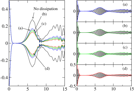
Figure 3: (Color online) Influence of the various dissipation mechanisms on the spontaneous revivals for a single qubit in the presence of a $\bar{n}=10$ photon field. The graph on the left depicts the analytical enveloppes for the Rabi oscillation signal $S^{z}(t)=P_{m=1/2}(t)-1/2$ as a function of $t/t_{R}$ for no dissipation (black lines), (a) only cavity dissipation $g/\kappa=840$, (b) cavity and qubit relaxation $g/\gamma_{1}=106$, (c) cavity relaxation and qubit pure dephasing $g/\gamma_{\varphi}=210$ and (d) all dissipation mechanisms present. The right part of the figure presents the associated Rabi oscillation signals obtained from quantum Monte-Carlo simulations (plain line) as well as the corresponding analytical enveloppes in cases (a) to (d).

Figure 4 compares the Rabi oscillation signals for the experimental parameters corresponding to Circuit QED lines in table 1. In cases (a) to (c), our anaytical model predicts the upper and lower enveloppes for the Rabi oscillation signal with good precision. But in case (d), only the initial collapse is correctly accounted for by the analytical enveloppes. Our Monte-Carlo simulation shows a relaxation of $S^{z}(t)$ towards $-1/2$ at longer times which is not described by our analytical model. This result is not surprising since for $g/\kappa=19.4$, at $t=5t_{R}$, the average photon number in the cavity should have decayed from 10 to 2 because of cavity relaxation alone. Therefore, at $t\sim 5t_{R}$, the qubit + cavity system is already out of the mesoscopic regime and our model is not expected to be valid in this regime.

Finally, these numerical and analytical results show that observing spontaneous Rabi oscillation revivals in circuit QED is not possible with the Circuit QED (1) parameters of table 1. Only the recent improvements on the value of $g/\kappa$ (Circuit QED (2) parameters) open the possibility for observing this phenomenon.

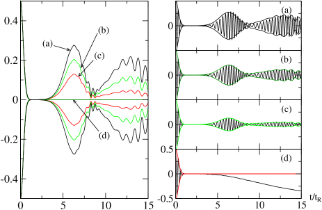
Figure 4: (Color online) Spontaneous revivals for a single qubit in the presence of a $\bar{n}=10$ photon field for various dissipative parameters. The graph on the left depicts the analytical enveloppes for the Rabi oscillation signal $S^{z}(t)=P_{m=1/2}(t)-1/2$ as a function of $t/t_{R}$ for (a) no dissipation, (b) Circuit QED (3) parameters, (c) Circuit QED (2) parameters and (d) Circuit QED (1) parameters (see table 1). The right part of the figure presents the associated Rabi oscillation signals obtained from quantum Monte-Carlo simulations (black lines) as well as the corresponding analytical enveloppes in cases (a) to (d).

The influence of photon number can be visualized through the effective decoherence coefficient $C(t,\bar{n})=|\mathcal{F}_{+-}(t)|$ as a function of $t/t_{R}=gt/2\pi$ and $\bar{n}$. It contains the effect of the environment on the contrast of Rabi oscillation revivals. Contour plots $C(t,\bar{n})=0.9$, $0.8$, $0.7$, $0.5$ and $0.2$ are shown on figure 5 for the Circuit QED parameter sets of table 1. The fourth graph shows these coutours for the case of a Rydberg atom experiment assuming a cavity damping time of 14 ms.

At high photon number, the various coutour curves tend to become vertical. This is easily understood by noticing that, at high photon number, the cavity decoherence coefficient becomes independant of $\bar{n}$ and dominated the decoherence process. In this regime, $C_{\kappa}(t)\simeq\exp{(-2\pi^{3}\,(g/\kappa)\,(t/t_{R})^{3})}$ and the decoherence time scales typically as $\pi t_{R}(2g/\kappa)^{1/3}$. Figure 5 shows that a coherent mesoscopic dynamics could be observed in really good conditions in cases (c) and (d): $C(t,\bar{n})\gtrsim 0.8$ at $t=t_{R}\sqrt{\bar{n}}$ corresponding to the generation of a mesoscopic field Schrődinger cat state involving up to 15 photons.

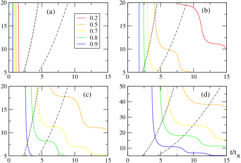
Figure 5: (Color online) Coutour plots of the effective decoherence coefficient $|\mathcal{F}_{+-}(t)|$ as a function of $t/t_{R}$ and $\bar{n}$ ($\bar{n}\geq 5$ to ensure validity of the mesoscopic approximation). The first three graphs represent the case of circuit QED devices: (a) Circuit QED (1) parameters, Circuit QED (2) parameters and (c) Circuit QED (3) parameters. Graph (d) depicts the corresponding information for Rydberg atom experiments with $g/\kappa=4310$ corresponding to a cavity with 14 ms damping time. In this case we extended the $\bar{n}$ range up to 50 photons. On each graph, the dashed line corresponds to the time of Schr dinger cat preparation $t=t_{R}\sqrt{\bar{n}}$ and the dot-dashed line correspond to the maximum of the first spontaneous Rabi oscillation revival $t=2t_{R}\sqrt{\bar{n}}$.

V.3 Echo experiment

First of all, we have considered a circuit QED echo experiment obtained with 10 photons initially and dissipative parameters $g/\kappa=840$, $g/\gamma_{1}=106$ and $g/\gamma_{\varphi}=210$ (Circuit QED (2) of table 1). Figure 6 shows the echo signals for $t/t_{R}=3$ as well as the analytical enveloppes obtained for $t=2t_{\pi}$ when the two quasi-coherent components of the field recombine.

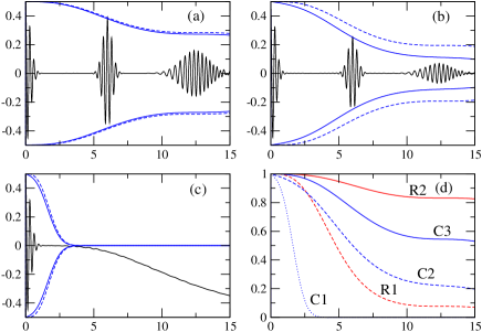
Figure 6: (Color online) Induced revivals signal $S^{z}(t)$ for one qubit in the presence of a $\bar{n}=10$ photon field for various dissipative paramerters as a function of $t/t_{R}$. Graphs (a) to (c) depict Rabi oscillation signals obtained from a quantum Monte-Carlo simulation for $t_{\pi}=3t_{R}$ (back curve). Analytical enveloppes showing the contrast at the induced revival $|\mathcal{F}_{+-}(t/2,t)|$ taking into account all sources of dissipation (full blue lines) or retaining only cavity relaxation (dashed blue lines) are also displayed. Graph (d) depicts the contrast of the induced revival as a function of $t/t_{R}=2t_{\pi}/t_{R}$ using parameters of table 1. The Circuit QED ($n$) parameter set corresponds to curve $Cn$ ($n=1$ to $3$) and the Rydberg atom ($m$) set parameter corresponds to curve $Rm$ ($m=1,2$).

Because the echo experiment reverses exactly the dyamics of the qubit + cavity system, the reduction of the induced Rabi oscillation revivals contrast is exactly given by the environmental decoherence: $C_{e}(t,\bar{n})=|\mathcal{F}_{+-}(t/2,t)|$. Figure 7 shows coutour plots for $C_{e}(t,\bar{n})$ as a function ot $t/t_{R}$ and $\bar{n}$ using the sets of parameters given in table 1 for circuit QED devices. As in the previous paragraph, the corresponding plot for Rydberg atom experiments with cavity damping time of 14 ms are given.

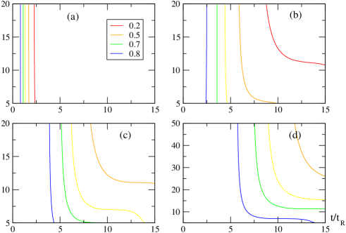
Figure 7: (Color online) Coutour plots of the effective echo decoherence coefficient $|\mathcal{F}_{+-}(t/2,t)|$ as a function of $t/t_{R}$ and $\bar{n}$ ($\bar{n}\geq 5$ to ensure validity of the mesoscopic approximation). The first three graphs represent the case of circuit QED devices: (a) Circuit QED (1) parameters, Circuit QED (2) parameters and (c) Circuit QED (3) parameters. Graph (d) depicts the corresponding information for Rydberg atom experiments with $g/\kappa=4310$ corresponding to a cavity with 14 ms damping time. In this case we extended the $\bar{n}$ range up to 50 photons.

V.4 Discussion of the results

Within the context of circuit QED experiments, our results suggest that tests of quantum coherence in the resonant mesoscopic regime could be performed using the latest generation of circuit QED devices. Echo experiments could be performed with up to 10 photons and echo times up to five vacuum Rabi periods. A more precise insight into the field dynamics could be obtained by performing a field tomography giving access to either the $Q$ or the Wigner function of the field. The $Q$ function probes the phase distribution of the field and its experimental determination would test the splitting of the field into two quasi-coherent components with opposite phases. Observing the induced revival then provides an experimental proof of the generation of a mesoscopic superposition superposition in the cavity Meunier et al. (2005).

On the other hand, Rydberg atom devices Raimond et al. (2001) are characterized by very long atomic relaxation time (33 ms) and the absence of atomic dephasing. The main limitation comes from cavity relaxation and time of flight. Up to 2005, the LKB team was able to work with a $\kappa^{-1}\simeq 1$ ms cavity relaxation time corresponding to $g/\kappa\simeq 310$ Meunier et al. (2005) (see row Rydberg atoms (1) in table 1). Cavity damping times up to 14 ms have been considered in our recent publication Meunier et al. (2006) an are recalled in row Rydberg atoms (2) of table 1. Recently, the LKB team reported on the realization of a ultra-high finesse cavity reaching $\kappa^{-1}\simeq 10$ Hz Kuhr et al. (2006) corresponding to $g/\kappa\simeq 31000$! With such performances, the only limitation is the atomic time of flight. This is an important limitation for the study of spontaneous revivals. In practice, only partial spontaneous revivals arising from small atomic ensembles could be observed Meunier et al. (2006). It is worth mentioning that circuit QED experiments do not suffer from this limitation although their dissipative properties are still behind the Rydberg atom ones.

VI Conclusion

Motivated by rapid experimental progresses of circuit QED devices, we have studied the dissipative dynamics of one qubit resonantly coupled to a mesoscopic field in a cavity taking into account cavity relaxation as well as qubit relaxation and pure dephasing. The resonant coupling between the qubit and the cavity produces an entangled state involving quasi-pointer states with respect to cavity relaxation. This very precise fact ultimately justifies in full generality the simple analytical model previously used to describe the dynamics of Rydberg atom ensembles coupled to a high-Q cavity Meunier et al. (2006). Although quasi-pointer states naturally produced by the resonant interaction are not preserved by qubit relaxation and dephasing, we have obtained a simple description of the dynamics of the cavity + qubit system in the presence of qubit dissipative processes. Simple analytical expressions for the spontaneous and induced Rabi oscillation signals have been obtained and shown and to be in good agreement with quantum Monte-Carlo simulations.

Our study shows that these effects and the generation of mesoscopic Schr dinger cat states could be within experimental reach in forthcoming circuit-QED experiments. However, our prediction may still be over optimistic since we did not attempt at modeling precisely the qubit readout. Thus, as done in Ref. Wallraff et al. (2005) for the Ramsey fringes measurement, the measurement beam can only be switched on after the qubit + cavity resonant interaction period, once the qubit has been sent off resonance for dispersive readout. Obtaining more precise quantitative results suitable for describing an actual experiment will probably require a more complete modeling of the experimental run, from preparation to measurement. The same remark is also relevant for obtaining precise predictions for the result of a cavity state tomography following for example a proposed protocol recently proposed in Ref. de Melo et al. (2006). Ultimately, we may probably have to rely on quantum Monte-Carlo simulations.

Other superconducting circuit for on-chip cavity QED have been proposed. In these proposals, the microstrip resonator is replaced by another oscillator such as an LC circuit or a biased large Josepshon junction in the appropriate parameter regime. Buisson and Hekking Buisson and Hekking (2001) have proposed a circuit that couples a current biased dc-SQUID to a Cooper pair box. In principle, values of $g/2\pi$ of the order of 100 to 200 MHz are within reach with such a device. However, modeling its dissipative dynamics requires taking into account the effect of low frequency noises which act on the qubit through low frequency dephasing and on the resonator through slow fluctuations of its resonant frequency. These effects are easy to account for using our formalism and a quasi-static approximation. But the resonator is also coupled to high frequency current noise through the SQUID Claudon et al. (2006). Work is in progress to describe the effect of this coupling on the Buisson-Hekking cavity-QED circuit.

Appendix A Non unitary evolution between quantum jumps

The non hermitian Hamiltonian describing the evolution between two quantum jumps is:

$$\hbar^{-1}H=\hbar^{-1}H_{JC}-\frac{i\gamma_{1}}{2}\,\frac{1+\sigma^{z}}{2}-\frac{\kappa}{2}\,N-i\frac{\gamma_{\varphi}}{4}$$ (39)

Obviously, the pure dephasing part leads to an trivial overall $e^{-\gamma_{\varphi}t/2}$ factor. In the mesoscopic regime, the resulting Hamiltonian can then be rewritten in terms of the $su(2)$ generators $\mathcal{J}^{a}$ suitable for describing the dynamics of generalized Gea-Banacloche states (3) Meunier et al. (2006):

$$\hbar^{-1}H_{\mathrm{eff}} = g\sqrt{p+1}\,\mathcal{J}^{x}-\frac{i\,\kappa}{2}\,p$$ (40)

$$- \frac{i\,(\gamma_{1}-\kappa)}{2}\,\mathcal{J}^{z}-\frac{i}{4}(\gamma_{1}+\kappa)\,.$$

This Hamiltonian is of the same form as the one discussed in appendix D of Meunier et al. (2006). The resulting dynamics can then be inferred straightforwardly. In Meunier et al. (2006), since $g\gg\kappa$, the backaction of cavity relaxation on the qubit has been neglected and since $g\ll\gamma_{1}$, the term proportional to $\gamma_{1}\mathcal{J}^{z}$ shall also be dropped out. Finally, starting from a state of the form

$$|\Psi(0)\rangle=e^{-\bar{n}/2}\sum_{p=0}^{\infty}\frac{\bar{n}^{p/2}}{\sqrt{p!}}\,|\Psi_{p}(0)\rangle$$

and assuming that $\gamma t\ll 1$, so that the average photon number in the cavity remains constant between $0$ and $t$, we get:

$$|\Psi_{{\mathrm{n.j.}}}(t)\rangle=e^{-\frac{(\gamma_{\varphi}+\gamma_{1})t}{4}}e^{-\frac{\kappa t}{2}}e^{-\bar{n}}\sum_{p=0}^{\infty}\frac{\bar{n}^{p/2}}{\sqrt{p!}}e^{-igt\sqrt{p+1}\mathcal{J}^{x}}\,|\Psi_{p}(0)\rangle\,.$$ (41)

The exponentially decaying prefactors are due to the non-hermiticity of the Hamiltonian. They reflect the decaying weight in time of quantum trajectories without any quantum jump between $0$ and $t$. The apparently surprising appearance of $\gamma_{1}/4$ instead of $\gamma_{1}/2$ for relaxation quantum jumps corresponds to time averaging to $1/2$ of the qubit populations induced by the strong coupling with the cavity. Physically, we assume that the number of photons is so high and relaxation so weak that the cavity mode keeps driving the qubit with the same intensity. Note that the resulting effective dynamics correspond to an effective Poissonian statistics of relaxation quantum jumps. But when the qubit state is close to $|-\rangle$, the probability rate for such a jump is much smaller than when it is close to $|+\rangle$. Indeed deviations from the effective Poissonian statistics average out since dissipative processes take place over a much longer time scale than rapid oscillations induced by the resonant qubit/cavity coupling.

Appendix B Effects of dissipation on the resonant cQED system

In this section, the evolution of generalized Gea-Banacloche states (3) under the stochastic dynamics involving qubit relaxation and dephasing is discussed. We first derive the effective dynamics resulting from relaxation and pure dephasing quantum jumps. The case of pure dephasing can then be treated exactly using renewal theory. A formal solution including relaxation in the low dissipation, large photon number limit is provided and used to extract the dominant contributions to the Rabi oscillation signal. This appendix provides a firm basis for the disscusions of sections IV.3 and IV.4.

B.1 Stochastic dynamics

B.1.1 Evolution of the coherences between generalized Gea-Banacloche states

In order to compute the evolution of the qubit + cavity state, it is convenient to look at the evolution of a coherence between a given pair of generalized Gea-Banacloche states with respective indices $(m_{+},m_{-})$. Such a coherence is initially of the form

$$\Pi_{m_{+},m_{-}}(0)=e^{-\bar{n}}\sum_{p_{+},p_{-}}\frac{\bar{n}^{(p_{+}+p_{-})/2}}{\sqrt{p_{+}!\,p_{-}!}}\,|X_{m_{+}}^{(p_{+})}\rangle\langle X_{m_{-}}^{(p_{-})}|\,.$$ (42)

As shown in appendix A, in the weak dissipation limit and in the mesoscopic regime, the evolution between quantum jumps is exactly the same as in the dissipationless case apart from the normalization prefactor that reflects the weight of quantum trajectories not presenting any quantum jump in the considered time interval. Moreoever, in the following, we shall restrict ourselved to short times ($\gamma t\ll 1$) so that the average photon number in the cavity remains constant. The effect of various quantum jumps is described by:

$$a\ldotp\,|X_{m}^{(p)}\rangle = \sqrt{p+1/2-m}\,|X_{m}^{(p)}\rangle$$ (43)

$$\sigma^{-}\ldotp\,|X_{\pm}^{(p)}\rangle = (|X_{+}^{(p-1)}\rangle-|X^{(p-1)}_{-}\rangle)/2$$ (44)

$$\sigma^{z}\ldotp\,|X_{m}^{(p)}\rangle = |X_{-m}^{(p)}\rangle\,.$$ (45)

In principle, we should follow keep track of all phases in each subspace generated by $|X_{\pm}^{(p)}\rangle$. It was proved in Ref. Meunier et al. (2006) that for cavity relaxation, this exact dynamics could be further simplified so that the resulting stochastic dynamics be expressed only in terms of the generalized Gea-Banacloche states (3). A similar route will be followed here and recasting eqs. (43) to (45) in terms of generalized Gea-Banacloche states using the mesoscopic approximation leads to:

$$a\ldotp|\Psi_{m}^{X}(\theta)\rangle = \sqrt{\bar{n}}\,e^{i\phi_{m,\theta}}\,|\Psi^{X}_{m}(\theta)\rangle$$ (46)

$$\sigma^{-}\ldotp|\Psi_{m}^{X}(\theta)\rangle = \frac{e^{i\phi_{m,\theta}}}{\sqrt{2}}\,\left(|\Psi^{X}_{+}(\theta)\rangle-|\Psi^{X}_{-}(-\theta)\rangle\right)$$ (47)

$$(i\sigma^{z})\ldotp|\Psi_{m}^{X}(\theta)\rangle = |\Psi^{X}_{-m}(-\theta)\rangle\,.$$ (48)

B.1.2 Trajectories of generalized Gea-Banacloche states

A sequence of quantum jumps of the above types will generate a tree structure whose vertices are associated with the branching expressed in eq. (47). Vertices associated with photons are located on straight edges of the tree and vertices associated with pure dephasing jumps are associated with direction reversals (see fig. 8). The state obtained from a given stochastic trajectory $\mathfrak{T}$ is a superposition of $2^{R_{\mathfrak{T}}}$ terms corresponding to all the paths along this tree structure where $R_{\mathfrak{T}}$ denotes the number of relaxation events along $\mathfrak{T}$ (see fig. 9 for an example where $\mathfrak{T}$ has two relaxation jumps, two dephasing jumps and two photon jumps). Note that each quantum jump $\alpha$ introduces a slow phase factor $\xi_{\alpha}$ depending on its type and its occurence time (see fig. 8). Finally, the state $|\Psi_{\mathfrak{T}}(t)\rangle$ associated with the quantum trajectory $\mathfrak{T}$ has the form:

$$|\Psi_{\mathfrak{T}}(t)\rangle=\sum_{\mathcal{T}\in\mathrm{Path}(\mathfrak{T})}\left(\prod_{0\leq t_{\alpha}\leq t}\xi_{\alpha}\right)\,|\Psi_{m^{\prime}_{t}}(\theta_{\mathcal{T}}(t))\rangle\,$$ (49)

where the sum in the r.h.s is performed over all paths $\mathcal{T}$ going downward the tree structure generated by quantum jumps along $\mathfrak{T}$ (black line in fig. 9). In this expression, $m^{\prime}_{t}=(-1)^{J[\mathcal{T}]}m$ depends on the number $J[\mathcal{T}]$ of direction changes along the path $\mathcal{T}$. The angle $\theta_{\mathcal{T}}(t)$ is related to the Fresnel angle $\phi_{\mathcal{T}}(t)$ by $\phi_{\mathcal{T}}(t)=-m^{\prime}_{t}\theta_{\mathcal{T}}(t)/2\sqrt{\bar{n}}$.

Figure 8: Tree structure associated with a stochastic trajectory with two photon emission, two pure dephasing quantum jumps and two relaxation jumps: (a) Vertices associated with the loss of a photon from the cavity (b) Vertices associated with a $\pi$ rotation of the qubit along the $z$ axis (pure dephasing) (c) Vertices associated with relaxation of the qubit in its ground state (relaxation).

Figure 9: The diagrammatic representation of a typical quantum stochastic trajectory $\mathfrak{T}$ showing two photon emissions from the cavity, two relaxations and two pure dephasing quantum jumps. Time would correspond to an horizontal axis whereas the vertical axis is the angle of the quasi generalized Gea-Banacloche state in the Fresnel plane. A single path $\mathcal{T}$ along $\mathfrak{T}$ is singularized (bold line).

B.1.3 Summing over stochastic trajectories

With this simple description of the stochastic dynamics, the evolution of the coherence (42) is of the form:

$$\Pi_{m_{+},m_{-}}(t)=\sum_{m^{\prime}_{+},m^{\prime}_{-}}\Pi^{(m^{\prime}_{+},m^{\prime}_{-})}_{m_{+},m_{-}}(t)$$ (50)

where $\Pi^{(m^{\prime}_{+},m^{\prime}_{-})}_{m_{+},m_{-}}(t)$ only involves coherence between the $|X_{m^{\prime}_{+}}^{(p)}\rangle$ and $|X_{m^{\prime}_{-}}^{(p)}\rangle$ states with $m^{\prime}_{\epsilon}=\pm m_{\epsilon}$. Explicitely

$$\Pi^{(m^{\prime}_{+},m^{\prime}_{-})}_{m_{+},m_{-}}(t) = e^{-\bar{n}}\sum_{p_{+},p_{-}}\frac{\bar{n}^{(p_{+}+p_{-})/2}}{\sqrt{p_{+}!\,p_{-}!}}$$ (51)

$$\times \mathcal{D}^{(p_{+},p_{-})}_{m^{\prime}_{+},m^{\prime}_{-}}(t)|X_{m^{\prime}_{+}}^{(p_{+})}\rangle\langle X_{m^{\prime}_{-}}^{(p_{-})}|$$

where the coefficient $\mathcal{D}^{(p_{+},p_{-})}_{m^{\prime}_{+},m^{\prime}_{-}}(t)$ (which will be denoted by $\mathcal{D}_{p_{+},p_{-}}(t)$ to shorten notation) is given by a path integral over all pairs of paths $\mathcal{T}_{\pm}$ downwards all possible pairs of quantum trajectories $\mathfrak{T}_{\pm}$ of the appropriate phase:

$$\mathcal{D}_{p_{+},p_{-}}(t) = \int\mathcal{D}[\mathcal{T_{+}},\mathcal{T_{-}}]\,S_{t}[\mathcal{T}_{+}]\times S_{t}[\mathcal{T}_{-}]^{*}$$ (52)

$$\times e^{2i\bar{n}(\sqrt{p_{+}+1}\phi_{\mathcal{T}_{+}}(t)-\sqrt{p_{-}+1}\phi_{\mathcal{T}_{-}}(t))}\,.$$

Here $S_{t}[\mathcal{T}_{\pm}]$ are the products taken along $\mathfrak{T}_{\pm}$ of slow phases appearing in eqs. (46) and (47):

$$S_{t}[\mathcal{T}_{\pm}]=\prod_{0\leq t_{\alpha_{\pm}}\leq t}\xi_{\alpha_{\pm}}\,.$$ (53)

B.1.4 Atomic observables

Let us assume that the atoms + cavity reduced density operator at time $t$ is of the form given by the r.h.s of (50). The Rabi oscillation signal is completely contained in the qubit polarization:

$$\langle\sigma^{z}(t)\rangle=e^{-\bar{n}}\sum_{p}\frac{\bar{n}^{p}}{p!}\,\frac{1}{2}\left(\mathcal{D}_{+-}^{(p,p)}(t)+\mathcal{D}_{-+}^{(p,p)}(t)\right)$$ (54)

and clearly involves the evolution of coherences between $|\Psi^{X}_{+}\rangle$ and $|\Psi^{X}_{-}\rangle$. Note however that it does not probe the coherence between subspaces associated with different values of $p$. The qubit coherence is given by:

$$\langle\sigma^{+}(t)\rangle = e^{-\bar{n}}\sum_{p}\frac{\bar{n}^{p}}{2\,p!}\,\frac{1}{2}\left(\mathcal{D}_{++}^{(p,p+1)}(t)-\mathcal{D}_{--}^{(p,p+1)}(t)\right.$$ (55)

$$+ \left.\mathcal{D}_{+-}^{(p,p+1)}(t)-\mathcal{D}_{-+}^{(p,p+1)}(t)\right)$$

and is sensitive to the coherence between adjacent multiplets.

B.2 Decoherence coefficients

The main problem is now to compute all decoherence coefficients $\mathcal{D}_{p_{+},p_{-}}(t)$ (which also depends on $m_{\pm}$ and $m^{\prime}_{\pm}$). As we shall see, this cannot be done exactly but a careful analysis of these sums in the mesoscopic regime will show us which trajectories contribute to the Rabi oscillation signal.

Generically, the decoherence coefficient $\mathcal{D}_{p_{+},p_{-}}(t)$ contains slow phases arising from the phase factors associated with photon emissions and qubit relaxations but also a rapid random phase $e^{2i\bar{n}\lambda_{p_{+},p_{-}}(\phi_{\mathcal{T_{+}}}-\phi_{\mathcal{T_{-}}})(t)}$ arising from difference of the eigenenergies of the states $|X^{(p_{\pm})}_{m_{\pm}}\rangle$. Note that in the absence of qubit relaxation and dephasing Meunier et al. (2006), this rapid phase is not random and therefore, decoherence is completely caused by the slow phases associated with photon losses of the cavity. Here, relaxation and dephasing quantum jumps of the qubit lead to the decay of $\mathcal{D}_{p_{+},p_{-}}(t)$. Indeed, in the mesoscopic regime, averaging of this rapid phase dominates the decay of the decoherence coefficient $\mathcal{D}_{p_{+},p_{-}}(t)$. To confirm this, let us consider the coefficient $D_{p_{+},p_{-}}(t)$ defined by forgetting slow phases in $\mathcal{D}_{p_{+},p_{-}}(t)$:

$$D_{p_{+},p_{-}}(t)=\int\mathcal{D}[\mathcal{T_{+}},\mathcal{T_{-}}]\,e^{2i\bar{n}(\sqrt{p_{+}+1}\phi_{\mathcal{T}_{+}}(t)-\sqrt{p_{-}+1}\phi_{\mathcal{T}_{-}}(t))}\,.$$ (56)

As we shall see now, this expression can be studied analytically by adapting renewal theory techniques already used to compute decoherence coefficients Schriefl et al. (2005).

B.2.1 Waiting time probabilities

The effective statistics of quantum jumps is Poissonian (see appendix A for relaxation) and statistics of jumps of different types are statistically uncorrelated. Equivalently, the probability distribution for waiting times between two jumps of type $j$ is exponential: $\psi_{j}(\tau)=\gamma_{j}\,e^{-\gamma_{j}\tau}$ where $\gamma_{\mathrm{cav}}=\bar{n}\kappa$, $\gamma_{\mathrm{deph}}=\gamma_{\varphi}/2$ and $\gamma_{\mathrm{relax}}=\gamma_{1}/2$. This exponential factor is taken into account through the norm of the states (41).

B.2.2 Pure dephasing

In this case, there are no slow phases and no branching. No approximation has been made beyond the mesoscopic approximation on the dissipationless problem. Hence we expect the following results to be valid even in the regime of strong dephasing $g\lesssim\gamma_{\varphi}$.

The decoherence coefficients $\mathcal{D}^{(p_{+},p_{-})}_{m^{\prime}_{+},m^{\prime}_{-}}(t)$ are given by averages over a telegraphic noise:

$$\mathcal{D}^{\mathrm{(e/o)}}_{\lambda}(t)=\langle e^{i\lambda\int_{0}^{t}X(\tau)\,d\tau}\rangle_{\mathrm{e}/\mathrm{o}}\,.$$ (57)

Here $\lambda=g(m_{+}\sqrt{p_{+}+1}-m_{-}\sqrt{p_{-}+1})$ and $X(\tau)=\pm 1$ is a telegraphic noise characterized by the probability distribution of waiting times between two switching $\psi(\tau)=(\gamma_{\varphi}/2)e^{-\gamma_{\varphi}\tau/2}$ and the initial condition $X(0)=1$. The $\mathrm{e}$ (respectively $\mathrm{o}$) symbol specifies that the average is performed over noise histories with an even (respectively odd) number of switchings between $0$ and $t$ ($m^{\prime}_{\pm}=m_{\pm}$ for the $\mathrm{e}$ case and $m^{\prime}_{\pm}=-m_{\pm}$ in the $\mathrm{o}$ case).

Renewal theory provides an elegant analytical solution for the decoherence coefficients (57). Introducing $\Pi_{0}(t)=\int_{t}^{\infty}\psi(\tau)\,d\tau$ and proceeding along the lines of Schriefl et al. (2004), the Laplace transforms of the $\mathcal{D}_{\lambda}^{\mathrm{(e/o)}}$ is obtained as:

$$L[\mathcal{D}_{\lambda}^{\mathrm{(e)}}](s) = \frac{L[\Pi_{0}](s+i\lambda)}{1-L[\psi](s-i\lambda)L[\psi](s+i\lambda)}$$ (58)

$$L[\mathcal{D}_{\lambda}^{\mathrm{(o)}}](s) = \frac{L[\Pi_{\lambda}](s)}{1-L[\psi](s-i\lambda)L[\psi](s+i\lambda)}$$ (59)

$$L[\Pi_{\lambda}](s) = \frac{L[\psi](s-i\lambda)\,(1-L[\psi](s+i\lambda))}{s+i\lambda}$$ (60)

Performing the inverse Laplace transform gives the explicit time dependence. The ”odd” coefficient is thus given by:

$$\mathcal{D}^{\mathrm{(o)}}(t)=\frac{\gamma_{\varphi}}{2(s_{+}-s_{-})}\,\left(e^{s_{+}t}-e^{s_{-}t}\right)$$ (61)

where

$$s_{\pm}=-\frac{\gamma_{\varphi}}{2}\pm i\sqrt{\lambda^{2}-\gamma_{\varphi}^{2}/4}\,.$$ (62)

The ”even” coefficient has a somehow more involved expression:

$$\mathcal{D}^{\mathrm{(e)}}_{\lambda}(t) = \frac{1}{2}\left(1-\frac{i\lambda}{s_{+}-s_{-}}\right)\,e^{s_{+}t}$$ (63)

$$+ \frac{1}{2}\left(1+\frac{i\lambda}{s_{+}-s_{-}}\right)\,e^{s_{+}t}\,.$$

Depending on the dimensionless coupling $\tilde{g}=2\lambda/\gamma_{\varphi}$, two distinct regimes occur.

For $\tilde{g}>1$, only a single event is enough to spread the phase significantly. Decoherence coefficients are dominated by noise histories with very low number of switching events. For $\mathcal{D}^{\mathrm{(e)}}_{\lambda}$, those are histories without any switwhing event whereas for $\mathcal{D}^{(o)}_{\lambda}$, histories with a single switching event dominate. In this strong dephasing limit $\tilde{g}\gg 1$, these expressions can be simplified

$$\mathcal{D}^{\mathrm{(e)}}_{\lambda}(t) = e^{-\gamma_{\varphi}t/2}\times e^{-i\lambda t}$$ (64)

$$\mathcal{D}^{\mathrm{(o)}}_{\lambda}(t) = \frac{\gamma_{\varphi}}{2\lambda}\,e^{-\gamma_{\varphi}t/2}\,\sin{(\lambda t)}\,.$$ (65)

In the $\tilde{g}\gg 1$ limit, only the ”even” contribution survives.

For $\tilde{g}\ll 1$, a large number of switching events is necessary to spread the phase $\lambda\int_{0}^{t}X(\tau)\,d\tau$ significantly. The dephasing time is then much longer than the typical waiting time. In this regime, we have:

$$\mathcal{D}^{(\mathrm{e}/\mathrm{o})}_{\lambda}(t)\simeq\frac{1}{2}\,e^{-\frac{\lambda^{2}}{\gamma_{\varphi}}\,t}$$ (66)

leading to a decoherence time of the order of $\gamma_{\varphi}/\lambda^{2}\gg\gamma_{\varphi}^{-1}$. Both coefficients are equal since having an even or an odd number of switchings makes no difference for $t\gg\gamma_{\varphi}^{-1}$.

In the present context, the coupling constant $\lambda$ depends on $p_{\pm}$ and $m_{\pm}$.

For $m_{+}\neq m_{-}$, we focus on the decoherence of a pair of generalized Gea-Banacloche states. In this case, for all values of $p_{\pm}$ close to $\bar{n}$, the dimensionless coupling is of the order of $\tilde{g}\simeq 2g\sqrt{\bar{n}}/\gamma_{\varphi}\gg 1$ meaning that we are in the $\tilde{g}\gg 1$ regime. In this case, formulas (64) and (65) are directly relevant and the decoherence rate is given by $\gamma_{\varphi}/2$.

For $m_{+}=m_{-}=m$, we focus on the decoherence of a single generalized Gea-Banacloche state. In this case, for $|p_{+}-p_{-}|\lesssim\sqrt{\bar{n}}$, the dimensionless coupling is then of the order of $\tilde{g}\simeq mg(p_{+}-p_{-})/\gamma_{\varphi}\sqrt{\bar{n}}$. Its smallest non zero value is reached for $|p_{+}-p_{-}|=1$: $mg/\gamma_{\varphi}\sqrt{\bar{n}}$. Therefore, for $\bar{n}\geq\bar{n}_{c}$ where $\bar{n}_{c}=(2g/\gamma_{\varphi})^{2}\gg 1$, the $\tilde{g}\ll 1$ limit can be reached for small enough $|p_{+}-p_{-}|$. On the other hand, the highest value is $\tilde{g}\simeq mg/\gamma_{\varphi}\gg 1$.

As long as $\bar{n}\ll\bar{n}_{c}$, which is the case of practical interest here, all decoherence coefficients $\mathcal{D}_{\lambda}(t)$ associated with $|p_{+}-p_{-}|\lesssim\sqrt{\bar{n}}$ are in the $\tilde{g}\gg 1$ regime. But for $\bar{n}\gg\bar{n}_{c}$, this is no longer the case. In this case, starting with a qubit initially in state $|X_{\pm}\rangle$, we find that the reduced density operator for the electromagnetic mode is of the form:

$$\rho_{\mathrm{cav}}(t)=e^{-\bar{n}}\sum_{p_{+},p_{-}}\frac{\bar{n}^{(p_{+}+p_{-})/2}}{\sqrt{p_{+}!\,p_{-}!}}e^{-\Gamma_{p_{+},p_{-}}t}\,|p_{+}\rangle\langle p_{-}|$$ (67)

where $\Gamma_{p_{+},p_{-}}$ is a rate bounded from above by $\gamma_{\varphi}$ and for sufficiently low $p_{+}-p_{-}$, given by:

$$\Gamma_{p_{+},p_{-}}\simeq\frac{\gamma_{\varphi}}{64}\,\left(\frac{\bar{n}_{c}}{\bar{n}}\right)\,(p_{+}-p_{p})^{2}\,.$$ (68)

The physical interpretation of these results is clear: the condition $\bar{n}\gtrsim\bar{n}_{c}$ means that the average number of dephasing jumps within the revival time $4\pi\sqrt{\bar{n}}/g$ is much larger than one. Since each of these jumps is equivalent to an echo pulse, the phase of the electromagnetic mode has a diffusive motion around zero thus leading to decoherence. In the end, the qubit, incoherent over times scales $\gtrsim\gamma_{\varphi}^{-1}$ due to its coupling with its own environment, tends to select specific states of the electromagnetic mode. These turn out to be Fock states. The fact that the coherence between adjacent Fock states decays over a much longer time scale than $\gamma_{\varphi}^{-1}$ (see (68)) reflects the time needed for a small incoherent object (the qubit) to decohere the mesoscopic coherent field.

To summarize, in the regime $g\ll\gamma_{\varphi}$ and $1\ll\bar{n}\ll\bar{n}_{c}$, the main contribution to the atoms + cavity reduced density operator comes from quantum trajectories without any quantum jump (decoherence coefficients $\mathcal{D}^{\mathrm{(e)}}_{\lambda}(t)$).

B.2.3 Qubit relaxation

Being primarily interested in the Rabi oscillation signals, we shall focus on the average value $\langle\sigma^{z}(t)\rangle$. Eq. (54) relates it to the coherences $|X_{+}^{(p)}\rangle\langle X_{-}^{(p)}|$ and $|X_{+}^{(p)}\rangle\langle X_{-}^{(p)}|$. Therefore it is sufficient to compute the decoherence coefficient $\mathcal{D}_{+-}^{(p,p)}(t)$. Because of the precise form of relaxation quantum jumps, it receives contributions from all four coefficients $\mathcal{D}_{\epsilon,\epsilon^{\prime}}^{(p,p)}(0)$. As a first guess, we might forget about the slow phases and compute approximate decoherence coefficients $D_{+-}^{(p,p)}$. In this case, the contribution of each pair of path is a well defined pure phase divided by $2^{R[\mathfrak{T}]}$ where $R[\mathfrak{T}]$ is the total number of relaxation jumps of the underlying quantum trajectory.

Consider now a specific pair of these paths $[\mathcal{T}_{+},\mathcal{T}_{-}]$. Since we are dealing with $p_{+}=p_{-}$, the phase accumulated between quantum jumps (duration $\Delta\tau$) is equal either to $e^{\pm ig\sqrt{p+1}\Delta\tau}$ when the two paths $\mathcal{T}_{+}$ and $\mathcal{T}_{-}$ are not parallel or to $1$ when they are parallel. Thus, one may conveniently associate with all $[\mathcal{T}_{+},\mathcal{T}_{-}]$ connecting to $|X_{-}^{(p)}\rangle\langle X_{+}^{(p)}|$ at time $t$ a 3-valued noise history: $X(\tau)\in\{0,\pm ig\sqrt{p+1}\}$ so that the pure phase associated with the pair of paths the is $\exp{(i\int_{0}^{t}X(\tau)\,d\tau)}$. Starting from the coherence $|X_{+}^{(p)}\rangle\langle X_{-}^{(p)}|$, there is one single pair of paths which connects to the same coherence and whose associated phase does not depend at all on the dates of quantum jumps occuring between $t=0$ and $t$. It consists into the pair of extremal paths depicted on fig. 10 and corresponds to $X(\tau)=g\sqrt{p+1}$. Any other pairs of paths will lead to a noise $X(\tau)$ presenting at least one blip, i.e. a time interval during which $X(\tau)\neq g\sqrt{p+1}$. Any other pair of paths starting from $|X_{+}^{(p)}\rangle\langle X_{-}^{(p)}|$ or any pair of paths starting from the diagonal terms $|X_{\epsilon}^{(p)}\rangle\langle X_{\epsilon}^{(p)}|$ ($\epsilon=\pm$) and ending on $|X_{+}^{(p)}\rangle\langle X_{-}^{(p)}|$ will exhibit an associated noise $\tau\mapsto X(\tau)$ that is not constant.

Figure 10: Plots of all pairs of trajectories involved in the evolution of the $|X_{-}\rangle\langle X_{+}|$ coherence having exactly two relaxation jumps. Relaxation jumps are shown as bifurcations. The $+$ and $-$ labels indicate which trajectories are relative to the forward and backward Keldysh contours. The extremal trajectories that dominate $\langle\sigma^{z}(t)\rangle$ are indicated with thick lines.

Given a certain noise history $\tau\mapsto X(\tau)$, we shall now sum over all pairs of trajectories $[\mathcal{T}_{+},\mathcal{T}_{-}]$ associated with a given function $\tau\mapsto X(\tau)$. One of them has a minimal number of relaxation jumps precisely occuring at the dates where $X(\tau)$ jumps. But of all histories having more relaxation jumps occuring between these specific dates must also be taken into account (this is an important difference with the case of pure dephasing studied in the previous paragraph). As shown in appendix A, the relaxation jumps stochastic process can be approximated by a renewal process with exponential waiting time distribution: $\psi_{R}(\tau)=\gamma\,e^{-\gamma\tau}$ where $\gamma=\gamma_{1}/2$. Taking into account the factor $1/2$ associated with each relaxation jumps, the resulting integration measure for intermediates times $(t_{1},\ldots,t_{p})$ where $0<t_{1}<\ldots<t_{p}<t$ is given by $d\mu(t_{1},\ldots,t_{p})=e^{-\gamma t/2}\,(\gamma/2)^{p}\,dt_{1}\ldots dt_{p}$. Note that the exponential factor $e^{-\gamma t}$ present in the waiting time distribution is partially compensated by the summation of all products of $1/2$ factors associated with relaxation jumps occuring at times different from the $t_{j}$s. The $1/2$ factors associated with jumps occuring at times $t_{j}$ are taken into account through $(\gamma/2)^{p}$.

This counting argument makes it clear that the contribution of paths associated with a non constant noise history will, comparatively to the case $X(\tau)=X(t)$, involve integrals of phases of the form $e^{ig\tau\sqrt{p+1}}$ or $e^{2ig\tau\sqrt{p+1}}$ over $\tau$ with measure $(\gamma/2)d\tau$, thus leading to a factor proportional to $\gamma/g\sqrt{p+1}$ which, in the mesoscopic regime, is or the order of $\gamma/g\sqrt{\bar{n}}$. Besides this, we are in the strong coupling regime and therefore $\gamma/g\sqrt{\bar{n}}$ is always much smaller than one. Thus, these contributions vanish in the regime considered in this paper.

Finally, our analysis shows that the dominant contribution to $\mathcal{D}_{+-}^{(p,p)}(t)$ in (52) comes from trajectories $\mathcal{T}_{\pm}$ for which the Fresnel angle $\phi_{\mathcal{T}_{\pm}}$ is monotonous in time. Of course, our argumentation ignored the slow phases that appear in (53) but it can be checked by explicit computation that our conclusion remains valid for pairs of paths with one or two jumps.

Retaining only the contribution of the pair of extremal paths in (52) and taking slow phases into account, the argumentation of Meunier et al. (2006) can then be straightforwardly adapted to resum their contribution along these trajectories. This immediatly leads to (28) where the $1/2$ prefactor in front of $e^{i(\Delta\phi)(\tau)}$ comes from the $1/2$ factor associated with each relaxation jump.

As a final comment, the above derivation also makes it clear that depending on the physical quantity we are interested in, other pairs of trajectories will contribute. As an example, computing the probability for having the qubit in the $|+\rangle$ or the $|-\rangle$ involves coefficients $\mathcal{D}^{(p,p)}_{++}$ $\mathcal{D}^{(p,p)}_{--}$ which are dominated by the sum over pair of paths such that $\mathcal{T}_{+}=\mathcal{T}_{-}$.

B.2.4 Summing over all dissipative processes

In the presence of dephasing, the extremal trajectories are still the dominant contribution to $\langle\sigma^{z}(t)\rangle$ and the effect of dephasing is an extra $e^{-\gamma_{\varphi}t/2}$ factor. Note that these corresponds to quantum histories without any dephasing quantum jump. These are expected to provide the dominant contribution in the low $\gamma_{\varphi}$ limit.

It follows from the previous analysis that the main contribution to $\langle\sigma^{z}(t)\rangle$ comes from pairs of extremal paths. Since photon losses are independant processes from relaxation jumps, their contribution can be computed using the formalism developped in Ref. Meunier et al. (2006). Obviously, it factors in front of the relaxation contribution. For $\kappa t\ll 1$, this enables to treat the regime where photon losses leading to decoherence of the generalized Gea-Banacloche states occur at a much higher rate than relaxation and pure dephasing $\kappa\bar{n}\gg\gamma_{1,\varphi}$.

References

- Brune et al. (1996a) M. Brune, E. Hagley, J. Dreyer, X. Maître, A. Maali, C. Wunderlich, J.M. Raimond, and S. Haroche, Phys. Rev. Lett. 77, 4887 (1996a).
- Blais et al. (2004) A. Blais, R.-S. Huang, A. Wallraff, S. M. Girvin, and R. J. Schoelkopf, Phys. Rev. A 69, 062320 (2004).
- Wallraff et al. (2004) A. Wallraff, D. I. Schuster, A. Blais, L. Frunzio, R.-S. Huang, J. Majer, S. Kumar, S. M. Girvin, and R. J. Schoekopf, Nature 431, 162 (2004).
- Wallraff et al. (2005) A. Wallraff, D. I. Schuster, A. Blais, L. Frunzio, J. Majer, M. H. Devoret, S. M. Girvin, and R. J. Schoelkopf, Phys. Rev. Lett. 95, 060501 (2005).
- Schuster et al. (2007) D. I. Schuster, A. A. Houck, J. A. Schreier, A. Wallraff, J.M. Gambetta, A. Blais, L. Frunzio, J. Mayer, B. Johnson, M. H. Devoret, S. M. Girvin, and R. J. Schoelkopf, Nature 445, 515 (2007).
- Gea-Banaloche (1991) J. Gea-Banacloche, Phys. Rev. A 44, 5913 (1991).
- Auffeves et al. (2003) A. Auffeves, P. Maioli, T. Meunier, S. Gleyzes, G. Nogues, M. Brune, J.M. Raimond, and S. Haroche, Phys. Rev. Lett. 91, 230405 (2003).
- Meunier et al. (2005) T. Meunier, S. Gleyzes, P. Maioli, A. Auffeves, G. Nogues, M. Brune, J.-M. Raimond, and S. Haroche, Phys. Rev. Lett. 94, 010401 (2005).
- Morigi et al. (2002) G. Morigi, E. Solano, B.-G. Englert, and H. Walther, Phys. Rev. A 65 040102(R) (2002).
- Meunier et al. (2006) T. Meunier, A. Le Diffon, C. Ruef, P. Degiovanni, and J.M. Raimond, Phys. Rev. A 74, 033802 (2006).
- Gea-Banacloche (1993) J. Gea-Banacloche, Phys. Rev. A 47, 2221 (1993).
- Dalibard et al. (1992) J. Dalibard, Y. Castin, and K. Molmer, Phys. Rev. Lett. 68, 580 (1992).
- Gambetta et al. (2006) J. Gambetta, A. Blais, D.I. Schuster, A. Wallraff, L. Frunzio, J. Majer, M.H. Devoret, S.M. Girvin, and R.J. Schoelkopf, Phys. Rev. A 74, 042318 (2006).
- Buisson and Hekking (2001) O. Buisson and F. Hekking, in Macroscopic quantum coherence and computing (Kluwer Academic Plenum Publishers New-York, 2001), p. 137.
- Jaynes and Cummings (1963) E. Jaynes and F. Cummings, Proc. IEEE 51, 89 (1963).
- Gleyzes et al. (2007) S. Gleyzes, S. Kuhr, C. Guerlin, J. Bernu, S. Deleglise, U. Busk Hoff, M. Brune, J.-M. Raimond, and S. Haroche, Nature 446, 297 (2007).
- Bertet et al. (2002) P. Bertet, A. Auffeves, P. Maioli, S. Osnaghi, T. Meunier, M. Brune, J.M. Raimond, and S. Haroche, Phys. Rev. Lett. 89, 200402 (2002).
- Brune et al. (1996) M. Brune, F. Schmidt-Kaler, A. Maali, J. Dreyer, E. Hagley, J.M. Raimond, and S. Haroche, Phys. Rev. Lett. 76, 1800 (1996).
- Maitre et al. (1997) X. Maitre, E. Hagley, G. Nogues, C. Wunderlich, P. Goy, M. Brune, J.M. Raimond, and S. Haroche, Phys. Rev. Lett. 79, 769 (1997).
- Klimov and Chumakov (1995) A. Klimov and S. Chumakov, Phys. Lett. A 202, 145 (1995).
- Frunzio et al. (2005) L. Frunzio, A. Wallraff, D. Schuster, J. Majer, and R. Schoelkopf, IEEE Transactions on Applied Superconductivity 15, 860 (2005).
- Makhlin et al. (2001) Y. Makhlin, G. Schőn, and A. Shmirman, Review of Modern Physics 73, 357 (2001).
- Koch et al. (2007) J. Koch, T. M. Yu, J. Gambetta, A. A. Houck, D. I. Schuster, J. Majer, A. Blais, M. H. Devoret, S. M. Girvin, and R. J. Schoelkopf (2007), URL http://arxiv.org/abs/cond-mat/0703002.
- Siddiqi et al. (2005) I. Siddiqi, R. Vijay, F. Pierre, C. M. Wilson, L. Frunzio, M. Metcalfe, C. Rigetti, R. J. Schoelkopf, M. H. Devoret, D. Vion, and D. Estève, Phys. Rev. Lett. 94, 027005 (2005).
- Astafiev et al. (2004) O. Astafiev, Y. A. Pashkin, Y. Nakamura, T. Yamamoto, and J. S. Tsai, Phys. Rev. Lett. 93, 267007 (2004).
- Makhlin and Shnirman (2003) Y. Makhlin and A. Shnirman, JETP Letters 78, 497 (2003).
- Vion et al. (2002) D. Vion, A. Aassime, A. Cottet, P. Joyez, H. Pothier, C. Urbina, D. Esteve, and M.H. Devoret, Science 296, 886 (2002).
- Makhlin and Shnirman (2004) Y. Makhlin and A. Shnirman, Phys. Rev. Lett. 92, 178301 (2004).
- Ithier et al. (2005) G. Ithier, E. Collin, P. Joyez, P. Meeson, D. Vion, D. Esteve, F. Chiarello, A. Shnirman, Y. Makhlin, J. Schriefl, et al., Phys. Rev. B 72, 134519 (2005).
- Kuhr et al. (2006) S. Kuhr, S. Gleyzes, C. Guerlin, J. Bernu, U. Busk Hoff, S. Deléglise, M. Brune, J.-M. Raimond, S. Haroche, S. Osnagi, et al. (2006), URL http://arxiv.org/abs/quant-ph/0612138.
- Paladino et al. (2002) E. Paladino, L. Faoro, G. Falci, and R. Fazio, Phys. Rev. Lett. 88, 228304 (2002).
- Blais et al. (2006) A. Blais, J. Gambetta, A. Wallraff, D. I. Schuster, S. M. Girvin, M. H. Devoret, and R. J. Schoelkopf, Phys. Rev. A 75, 032329 (2007).
- Raimond et al. (2001) J. Raimond, M. Brune, and S. Haroche, Rev. Mod. Phys. 73, 565 (2001).
- de Melo et al. (2006) F. de Melo, L. Aolita, F. Toscano, and L. Davidovich, Phys. Rev. A 73, 030303(R) (2006).
- Claudon et al. (2006) J. Claudon, A. Fay, L.P. Levy, and O. Buisson, Phys. Rev. B 73, 180502(R) (2006).
- Schriefl et al. (2005) J. Schriefl, M. Clusel, D. Carpentier, and P. Degiovanni, Phys. Rev. B 72, 035328 (2005).
- Schriefl et al. (2004) J. Schriefl, M. Clusel, D. Carpentier, P. Degiovanni, and Y. Makhlin, in Quantum information and decoherence in nanosystems, edited by C. Glattli, T. Martin, B. Pannetier, and M. Sanquer (2004).