Time scale competition leading to fragmentation and recombination transitions
in the co-evolution of network and states.

Abstract

We study the co-evolution of network structure and node states in a model of multiple state interacting agents. The system displays two transitions, network recombination and fragmentation, governed by time scales that emerge from the dynamics. The recombination transition separates a frozen configuration, composed by disconnected network components whose agents share the same state, from an active configuration, with a fraction of links that are continuously being rewired. The nature of this transition is explained analytically as the maximum of a characteristic time. The fragmentation transition, that appears between two absorbing frozen phases, is an anomalous order-disorder transition, governed by a crossover between the time scales that control the structure and state dynamics.

I Introduction

Recent findings in the topological characterization of real complex networks have triggered a theoretical understanding of diverse complex systems. A great deal of effort has been devoted to the modelling of complex networks from a topological point of view, and to the dynamics on different classes of networks Albert02 . In the latter, the evolution of the states of the nodes is usually assumed much faster that the time characterizing the network dynamics. Less effort has been devoted to the understanding of the entangled co-evolution of network structure and state dynamics, i.e., how the structure of a network affects the dynamics on it and vice versa. For instance in a social system, individuals shape their opinions depending on their neighbors’ opinions, but simultaneously, the individuals’ opinions affect with whom they interact Skyrms00 ; Zimmermann04 ; Marsili04 ; Eguiluz05b ; Gil06 ; Holme07 . The network of interactions co-evolve with the dynamics of opinions.

The influence of network topology has been analyzed extensively for several models of consensus formation Suchecki05 ; Sanmiguel05 . A main question is related to the mechanisms and network topologies that lead to consensus, i.e., all agents having the same state. Based on social pressure, how state changes, and homophily, the tendency of individuals to interact with similar others, the Axelrod model Axelrod97 represents a paradigmatic model displaying an order-disorder nonequilibrium transition Castellano00 . When the network of interaction is regular, random or small-world, the system orders if the degree of initial disorder is below a critical value Castellano00 ; Klemm03a ; Klemm03b ; Vazquez07 . In the ordered phase, a domain (set of connected agents with the same state) of the order of the system size spans the network, while in the disordered phase, many small domains are formed. Motivated by the mechanisms of social pressure and homophily, in this paper we analyze the co-evolution in the Axelrod model between the network of interactions and the state dynamics of the nodes, by allowing interaction links to be rewired depending on the state of the agents at their ends.

II The model

A population of $N$ agents are located at the nodes of a network. The state of an agent $i$ is represented by an $F$-component vector $\sigma_{if}$, $f=1,2,\ldots,F$, and $i=1,2,\ldots,N$, where each component represents an agent’s attribute. There are $q$ different choices or traits per feature, labelled with an integer $\sigma_{if}\in\{0,\ldots,q-1\}$, giving raise to $q^{F}$ possible different states.

Initially agents take one of the $q^{F}$ states at random. In a time step an agent $i$ and one of its neighbors $j$ are randomly chosen:

1. If the agents share $m>0$ features, they interact with probability equal to the fraction of shared features, i.e., the overlap ($m/F$). In case of interaction, an unshared feature is selected at random and $i$ copies $j$’s value for this feature.

2. If the agents do not share any feature, then $i$ disconnects its link to $j$ and connects it to a randomly chosen agent that $i$ is not already connected to.

Step $1$ describes the original Axelrod dynamics: Alike agents become even more similar as they interact, increasing the probability of future interaction. Step $2$ implements the network co-evolution: incompatible agents, i.e., agents with no features in common, tend to get disconnected. We have performed extensive numerical simulations to study the behavior of the system as the control parameter $q$ is varied, for different population sizes $N$, number of features $F=3$, and starting from a random network with average degree $\langle k\rangle=4$. The results do not depend on the initial network topology, because the repeated rewiring dynamics leads to a random network with a Poisson degree distribution.

The model displays two transitions, both very different in nature. The first one is an order-disorder transition at $q=q_{c}$ between two frozen phases, associated with the fragmentation of the network. The dynamics leads to the formation of network components, where a component is a set of connected nodes. In a frozen configuration agents that belong to the same component have the same state. For $q<q_{c}$ (ordered phase I), the system reaches a configuration composed by a giant component of the order of the system size, and a set of small components; for $q>q_{c}$ (disordered phase II) the large component disintegrates in many small disconnected components. The second transition, related with network recombination, occurs at $q=q^{*}$ between the phase II and an active phase III, where the system reaches a dynamic configuration with links that are permanently rewired.

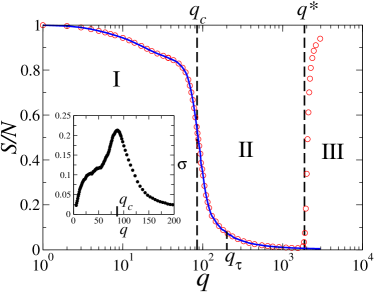
Figure 1: Average relative size of the largest network component (circles) and largest domain (solid line) in the stationary configuration vs $q$, for $N=2500$, averaged over $400$ realizations. The vertical lines at $q_{c}=85$ and $q^{*}=1875$ indicate the transition points between the different phases. Inset: fluctuations are maximum at the critical point $q_{c}$.

III Frozen phases (I and II)

For small values of $q$ in phase I, the average size of the largest network component $S$ in the final configuration is of the order of the system size $N$ (Fig. 1), due to the high initial overlap between the states of neighboring agents. As $q$ increases inside phase I, the initial overlap decreases and $S$ also slowly decreases. For larger values of $q$ (phase II), many distinct domains are formed initially inside the components which break into many small disconnected components and, as a result, $S$ reaches a value much smaller than $N$ (network fragmentation). During the evolution of the system, a network component can have more than one domain. However, in the final configuration of phases I and II, one component corresponds to one domain.

The transition point from phase I to phase II is defined by the value $q=q_{c}$ for which the fluctuations in $S$ reach a maximum value. This value corresponds to the point where the order parameter $S$ suffers a sudden drop. For $N=2500$ we find $q_{c}=85\pm 2$ (see Fig. 1). To further investigate this transition point we calculated the size distribution of network components $P(s)$ (see Fig. 2). For small $q$, $P(s)$ shows a peak that corresponds to the average size of the largest component $S$, and has an exponential decay corresponding to the distribution of small disconnected components. The peak at $S$ decreases as $q$ increases, giving raise to a power law decay of $P(s)$ at $q_{c}\simeq 85$, a signature of a transition point Stauffer92 ; Klemm03a .

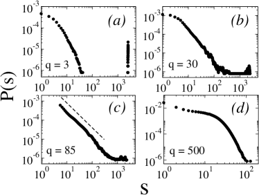
Figure 2: Size distribution of network components for $N=2500$ and values of $q$ (a,b) below, (c) at, and (d) above the transition point $q_{c}\simeq 85$. The dashed line represents a power law with exponent $-1.3\pm 0.02$.

The behavior of the order parameter $S/N$ depends on system size (Fig. 3). When both axis are rescaled by $N^{-\alpha}$ with $\alpha=0.82\pm 0.01$ the data collapses for $q$ smaller than $q_{c}$. This implies that $q_{c}$ increases with the system size $N$ as $q_{c}\sim N^{\alpha}$, and suggests a scaling relation for $S$ in the ordered phase $S=N^{\alpha}f(N^{-\alpha}q)$, where $f(\cdot)$ is a scaling function. The scaling relation implies that the discontinuity disappears in the large $N$ limit. Thus, not only the transition point diverges as $q_{c}\sim N^{~{}0.82}$ but also the amplitude of the order parameter $S/N\sim N^{-0.18}$ vanishes as $N$ goes to infinity.

These results, maximum of the fluctuations, data collapse and distribution of component sizes, identify $q_{c}$ as the critical point of the transition. The fact that the exponent of the size distribution is smaller than $2$ and that the discontinuity of the order parameter tends to $0$ as system size increases, suggest that in the large $N$ limit the transition becomes continuous with $q_{c}\to\infty$.

IV Active phase (III)

We analyze this phase by looking at the rewiring dynamics. A link that connects a pair of incompatible agents is randomly rewired until it connects two compatible agents, i.e., agents with at least one feature in common. If the number of pairs of compatible agents $L_{c}$ is larger than the total number of links in the system $\langle k\rangle N/2$, this rewiring process continues until all links connect compatible agents. Later, the system evolves until each component constitutes a single domain, the frozen configurations reached in phases I and II. If, on the contrary, $L_{c}$ gets smaller than $\langle k\rangle N/2$, the system evolves connecting first all $L_{c}$ pairs by links. The state dynamics stops when no further change of state is possible, but the rewiring dynamics continues for ever with approximately $\langle k\rangle N/2-L_{c}$ links that repeatedly fail to attach compatible agents. This is the active configuration observed in phase III. Thus, in contrast to phases I and II, in the stationary configurations of phase III there are typically more than one domain per component. The size of the largest component abruptly increases at $q^{*}$ indicating that a giant component reappears (network recombination), while the size of the largest domain continues decreasing (see Fig. 1).

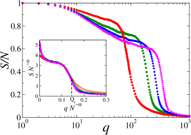
Figure 3: Average relative size of the largest network component $S/N$ vs $q$ for system sizes $N=2500$, $6400$, $10000$ and $14400$ (left to right), averaged over $400$ realizations. Inset: Finite size scaling. The data collapses below the scaled transition point $Q_{c}=q_{c}N^{-\alpha}$, with $\alpha=0.82$.

To estimate $q^{*}$, we will assume $L_{c}$ constant during the evolution as for $q$ large the state of the agents does not evolve much. Thus, with the ansatz $L_{c}\simeq L_{c}(t=0)\simeq\frac{N(N-1)}{2}\left[1-(1-1/q)^{F}\right]\simeq N^{2}F/2q$, for $q\gg F$ and
$N\gg 1$, the condition at the transition point is $N^{2}F/2q^{*}\simeq\langle k\rangle N/2$, so that

$$q^{*}\simeq\frac{NF}{\langle k\rangle}~{}$$ (1)

is the value of the recombination transition point. For the values considered here we obtain $q^{*}=1875$ in good agreement with the numerical results (Fig. 1).

V Dynamic time scales

In order to understand the final structure of the network in phases I and II we analyzed the time evolution of the nodes’ states and interaction links. In Fig. 4 we plot the time evolution of the density of network components, $n_{c}=$ number of components$/N$, and domains, $n_{d}=$number of domains$/N$, averaged over $1000$ realizations, and for three values of $q$. An interesting quantity is the average time to reach the final frozen configuration $\tau$. If $\tau_{d}$ [$\tau_{c}$] is the average time at which $n_{d}$ [$n_{c}$] reaches its stationary value, then $\tau$ is largest between $\tau_{d}$ and $\tau_{c}$ (see Figs. 4 and 5). The curves for $\tau_{d}$ and $\tau_{c}$ as a function of $q$ cross at a value $q_{\tau}$ (Fig. 5). As we shall see, $q_{\tau}$ identifies a transition between two different dynamic regimes for the formation of domains and network components, that lead to the frozen configurations observed in phases I and II (Figs. 4 and 5).

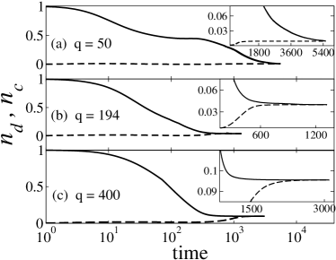
Figure 4: Time evolution of the density of domains $n_{d}$ (solid line) and network components $n_{c}$ (dashed line), for $N=2500$ and values of $q$ (a) below, (b) at, and (c) above the transition point $q_{\tau}=194\pm 10$. Each inset is a zoom of the region that shows the approach to the final configuration.

For $q<q_{\tau}$, the dynamics causes the network to break into a giant component and small components. Due to the initial overlap between the states of the agents inside each component, the network stops evolving at a time $\tau_{c}$ where $n_{c}$ reaches its stationary maximum value (see Fig. 4a). After this stage, domains compete inside each component, until only one domain occupies each component. The approach to the frozen configuration is controlled by the coarsening process inside the largest component, whose structure is similar to a random network due to the random rewiring dynamics. Then, given that the dynamics of the last and longest stage before reaching consensus inside this component is governed by interfacial noise as in the voter model Klemm03c , $\tau$ is expected to scale as the size of the largest component $\tau\sim S$ Sood05 .

For $q>q_{\tau}$, there is a transient during which $n_{d}$ decreases, indicating that, in average, domains grow in size (see Fig. 4c). At time $\tau_{d}$, $n_{d}$ reaches a stationary value when the overlap between distinct domains is zero. At this stage domains are still interconnected by links between incompatible agents. As domains progressively disconnect from each other $n_{c}$ increases. When finally the links connecting incompatible agents disappear all domains get fragmented, $n_{c}$ equals $n_{d}$ and the system reaches its final configuration in a time $\tau=\tau_{c}$.

At $q_{\tau}$, the time scale governing the state dynamics is the same as the time scale governing the network dynamics $\tau_{d}=\tau_{c}$ (Figs. 4b,5). Thus, it indicates that the ordered phase I is dominated by a slower state dynamics on a network that freezes on a fast time scale, while in the disordered phase II the state dynamics freezes before the network reaches a final frozen configuration. Even though $q_{\tau}$ is found to be larger than the critical point $q_{c}$, the relative difference between $q_{\tau}$ and $q_{c}$ decreases with $N$ (inset of Fig. 5), suggesting that both transition points become equivalent in the large $N$ limit. Thus, the competition between the time scales $\tau_{d}$ and $\tau_{c}$ governs the fragmentation transition at $q_{c}$.

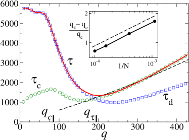
Figure 5: Convergence times $\tau_{c}$ (circles), $\tau_{d}$ (squares) and $\tau$ (solid line) vs $q$ for $N=2500$ and averaged over $500$ configurations. The result from Eq. (5) (dashed line) is compared with $\tau$ and $\tau_{c}$ for $q>q_{\tau}=194\pm 10$. Inset: relative difference between the transition points $q_{\tau}$ and $q_{c}$ vs $1/N$ in log-log scale. The dashed line has slope $0.30\pm 0.01$.

In the remainder, we derive an approximate expression for $\tau$ in phase II by studying the decay of the number of links between incompatible agents $N_{0}$. We shall see that this approach unveils the transition from the frozen to the active phase, leading to the transition point $q^{*}$.

In the continuum time limit, and neglecting the creation of incompatible links, $N_{0}$ decays according to the equation:

$$\frac{dN_{0}}{dt}\simeq-\frac{1}{\frac{1}{N}}\frac{2N_{0}}{\langle k\rangle N}\frac{N_{c}}{N}=-\frac{2N_{0}\;N_{c}}{\langle k\rangle N}.$$ (2)

In a time step $\Delta t=\frac{1}{N}$, an incompatible link $(i,j)$ is chosen with probability $\frac{2N_{0}}{\langle k\rangle N}$. One of its ends $j$ is moved to a random node $k$. The probability that $k$ is compatible to $i$ is $\frac{N_{c}}{N}$, where $N_{c}$ is the number of compatible agents to $i$ but still not connected to $i$. In a mean-field spirit, every node has $\langle k\rangle$ edges that need to be connected to $\langle k\rangle$ different compatible agents. We approximate $N_{c}$ as the average number of compatible agents per agent. When $i$ attaches an edge to a compatible agent, $N_{0}$ is reduced by one while $N_{c}$ is reduced by $2/N$ given that both $i$ and $k$ loose a compatible partner. Assuming that the set of compatible agents to $i$ remains the same we write $N_{c}\simeq\frac{2N_{0}}{N}+A$, where $A=N_{c}(0)-\frac{2N_{0}(0)}{N}\simeq\frac{NF}{q}-\langle k\rangle$ for $N\gg 1$ and $q\gg F$. Substituting this last expression for $N_{c}$ into Eq. (2) and rewriting it in terms of the transition point $q^{*}=NF/\langle k\rangle$ we obtain

$$\frac{dN_{0}}{dt}\simeq-\frac{2N_{0}}{\langle k\rangle N}\left(\frac{2N_{0}}{N}+\frac{\langle k\rangle}{q}\left(q^{*}-q\right)\right).$$ (3)

Equation (3) has two stationary solutions. For $q<q^{*}$, the steady configuration is $N_{0}^{S}=0$, corresponding to the frozen phases I and II, while for $q>q^{*}$ the stationary solution $N_{0}^{S}=\frac{\langle k\rangle N}{2q}(q-q^{*})$ corresponds to the active phase III. We recover our previous result that for $q>q^{*}$ the system reaches a stationary configuration with a constant fraction of links $N_{0}$ larger than zero, that are permanently rewired. Therefore, the system never freezes. Note that in the limit of very large $q$, all agents are initially incompatible, consequently $N_{0}$ approaches to the total number of links $\frac{1}{2}\langle k\rangle N$.

Integrating Eq. (3) by a partial fraction expansion gives

$$t=\frac{qN}{2(q^{*}-q)}\ln\left[\frac{q+\frac{\langle k\rangle N}{2N_{0}(t)}(q^{*}-q)}{q^{*}}\right].$$ (4)

For $q<q^{*}$, the system freezes at a time $\tau$ at which $N_{0}\simeq 1$, thus

$$\tau\simeq\frac{qN}{2(q^{*}-q)}\ln\left[\frac{q+\frac{1}{2}\langle k\rangle N(q^{*}-q)}{q^{*}}\right]~{},\mbox{~{}for~{}}q_{\tau}<q<q^{*}.$$ (5)

This result is in agreement with the numerical solution (Fig. 5).

For $q>q^{*}$, the system reaches a stationary configuration. Thus we define $\tau$ as the time at which $N_{0}\simeq\frac{\langle k\rangle N}{2q}(q-q^{*})+1$, then

$$\tau\simeq\frac{qN}{2(q^{*}-q)}\ln\left[\frac{2q^{2}}{q^{*}(\langle k\rangle N(q-q^{*})+2q)}\right]~{},$$ (6)

for $q^{*}<q<\frac{N^{2}F}{2}$. $\tau$ decreases with $q$ and it vanishes for $q>N^{2}F/2$ where initially all pairs of nodes are incompatible, thus the system starts from a stationary configuration, giving $\tau=0$ for $q>\frac{N^{2}F}{2}$.

From Eqs. (5) and  (6) we obtain that $\tau$ reaches a maximum value equal to $\frac{1}{4}\langle k\rangle N^{2}$ at $q=q^{*}$; an indication of the transition.

VI Summary and Conclusions

We have studied the Axelrod model with co-evolution of the interaction network and state dynamics of the agents. The interplay between structure and dynamics gives rise to two different transitions. First, a recombination transition between a frozen and an active phase. The characteristic time to reach a stationary configuration shows a maximum at the transition point between these two phases. Second, an order-disorder transition associated with network fragmentation that appears at a critical value $q_{c}$ where the component size distribution follows a power-law. Finite size scaling analysis suggests that in the large $N$ limit this transition becomes continuous with $q_{c}$ going to infinity. The fragmentation is shown to be a consequence of the competition between two coupled mechanisms, network formation and state formation. These mechanisms are governed by two internal time scales, $\tau_{c}$ and $\tau_{d}$ respectively, which are not controlled by external parameters, but they emerge from the dynamics. For $q<q_{c}$ the network components, that are formed first, control the formation of states. For $q>q_{c}$ the fast formation of domains shape the final structure of the network.

An important aspect of the co-evolution is that the network evolution is coupled to the state of the agents, in contrast to other models where the links are severed, reconnected and/or appear as a random process independent of the state of the nodes. The robustness of the fragmentation and recombination in the presence of noise should also be considered Centola06 . Our results provide a simple mechanism, co-evolution, that could explain the community structure found in general in the analysis of complex networks, and in particular of social systems Palla07 where this mechanism can be understood in terms of network homophily Centola06 .

- (1) R. Albert and A.-L. Barabási, Rev. Mod. Phys. 74, 47 (2002).
- (2) B. Skyrms and R. Pemantle, Proc. Natl. Acad. Sci. USA 97, 9340 (2000).
- (3) M.G. Zimmermann, V.M. Eguíluz, and M. San Miguel, Phys. Rev. E 69, 065120(R) (2004).
- (4) M. Marsili, F. Vega-Redondo, and F. Slanina, Proc. Natl. Acad. Sci. USA 101, 1439 (2004).
- (5) V.M. Eguíluz, M.G. Zimmermann, C.J. Cela-Conde, and M. San Miguel, Am. J. Sociol. 110, 977 (2005).
- (6) S. Gil and D.H. Zanette, Phys. Lett. A 356, 89 (2006).
- (7) P. Holme and M.E.J. Newman, Phys. Rev. E 74, 056108 (2006).
- (8) M. San Miguel, V.M. Eguíluz, R. Toral, and K. Klemm, Comput. Sci. Eng. 7, 67 (2005).
- (9) K. Suchecki, V.M. Eguíluz, and M. San Miguel, Europhys. Lett. 69 228 (2005);Phys. Rev. E 72, 036132 (2005).
- (10) R. Axelrod, J. Conflict Res. 41, 203 (1997)
- (11) C. Castellano, M. Marsili, and A. Vespignani, Phys. Rev. Lett. 85, 3536 (2000).
- (12) K. Klemm, V.M. Eguíluz, R. Toral, and M. San Miguel, Phys. Rev. E 67, 026120 (2003).
- (13) K. Klemm, V.M. Eguíluz, R. Toral, and M. San Miguel, Physica A 327, 1 (2003).
- (14) F. Vazquez and S. Redner, Europhys. Lett. 78, 18002 (2007).
- (15) D. Stauffer and A. Aharony, Introduction to percolation theory (Taylor and Francis, London, 1992).
- (16) K. Klemm, V.M. Eguíluz, R. Toral, and M. San Miguel, Phys. Rev. E 67, 045101(R) (2003).
- (17) V. Sood and S. Redner, Phys. Rev. Lett. 94 178701 (2005).
- (18) D. Centola, J.C. González-Avella, V.M. Eguíluz, and M San Miguel, physics/0609213.
- (19) G. Palla, A.-L. Barabási, and T. Vicsek, Nature (London) 446, 664 (2007).