Invertible harmonic mappings, beyond Kneser

Abstract.

We prove necessary and sufficient criteria of invertibility for planar harmonic mappings which generalize a classical result of H. Kneser, also known as the Radó–Kneser–Choquet theorem.

1. Introduction

Let $B:=\{(x,y)\in\mathbb{R}^{2}:x^{2}+y^{2}<1\}$ denote the unit disk. Given a homeomorphism $\Phi$ from the unit circle $\partial B$ onto a simple closed curve $\gamma\subseteq\mathbb{R}^{2}$, let us consider the solution $U\in C^{2}(B;\mathbb{R}^{2})\cap C(\overline{B};\mathbb{R}^{2})$ to the following Dirichlet problem

(1.1) $$\left\{\begin{array}[]{lll}\Delta U=0,&\hbox{in}&B,\\ U=\Phi,&\hbox{on}&\partial B.\end{array}\right.$$

The basic question that we address in this paper is under which conditions on $\Phi$ we have that $U$ is a homeomorphism of $\overline{B}$ onto $\overline{D}$, where $D$ denotes the bounded open, simply connected set for which $\partial D=\gamma$.

The fundamental benchmark for this issue is a classical theorem, first conjectured by T. Radó in 1926 [16], which was proved immediately after by H. Kneser [12], and subsequently rediscovered, with a different proof, by G. Choquet [7]. Let us recall the result.

Theorem 1.1 (H. Kneser).

If $D$ is convex, then $U$ is a homeomorphism of $\overline{B}$ onto $\overline{D}$.

We recall that this Theorem had a remarkable impact in the development of the theory of minimal surfaces, see for instance [17]. Its influence appears also in other areas of mathematics, let us mention here homogenization and effective properties of materials [5, 2, 3], inverse boundary value problems [10, 1, 11] and, quite recently, variational problems for maps of finite distortion [4]. See also, as general references, and for many interesting related results, the book by Duren [9] and the review article by Bshouty and Hengartner [6].

The amazing character of Kneser’s Theorem stands in the simplicity and elegance of the geometric condition on the target curve $\gamma$. Let us emphasize here that this condition does not involve the choice of the parametrization $\Phi$ of the curve $\gamma$.

In order to motivate the main result of this paper, Theorem 1.3 below, we wish to stress that no weaker condition on the shape of $D$ can replace the assumption in Theorem 1.1. In fact, the following Theorem holds.

Theorem 1.2 (G. Choquet).

For every Jordan domain $D$ which is not convex, there exists a homeomorphism $\Phi:\partial B\to\partial D$ such that the solution $U$ to (1.1) is not a homeomorphism.

A proof for this Theorem is due to Choquet [7, §3]. In Section 6 we present a new proof aimed at having a more explicit description of the homeomorphism $\Phi$. In the final part of this Introduction, when presenting the content of Section 6, we shall illustrate the advantages of this new proof with more details.

Theorem 1.2 shows that, given a non–convex domain $D$ and its boundary $\gamma$, one can find some parameterization of the latter which give rise to a non–invertible solution to (1.1). On the other hand, by the Riemann Mapping Theorem, see for instance [15, Theorem 3.4], for any such $\gamma$ one can also find other parameterizations for which the corresponding solution to (1.1) is a homeomorphism and, in fact, a conformal mapping. Thus the question arises, for a given simply connected target domain $D$, possibly non–convex, of how to characterize all the parameterizations which give rise to an invertible solution to (1.1).

Our main result is a complete answer to this question for those parameterizations $\Phi$ which are smooth enough so that the corresponding solution to (1.1) belongs to $C^{1}(\overline{B};\mathbb{R}^{2})$.

Theorem 1.3.

Let $\Phi:\partial B\to\gamma\subset\mathbb{R}^{2}$ be an orientation preserving diffeomorphism of class $C^{1}$ onto a simple closed curve $\gamma$. Let $D$ be the bounded domain such that $\partial D=\gamma$. Let $U\in C^{2}(B;\mathbb{R}^{2})\cap C(\overline{B};\mathbb{R}^{2})$ be the solution to (1.1) and assume, in addition, that $U\in C^{1}(\overline{B};\mathbb{R}^{2})$.

The mapping $U$ is a diffeomorphism of $\overline{B}$ onto $\overline{D}$ if and only if

(1.2) $$\begin{array}[]{lll}\det DU>0&\hbox{everywhere on}&\partial B.\end{array}$$

Remark 1.4.

In order to compare this statement with Kneser’s Theorem, it is worth noticing that, when $\gamma$ is convex, (1.2) is automatically satisfied. Indeed we shall prove, see Lemma 5.3, that $\det DU>0$ always holds true on the points of $\partial B$ which are mapped through $\Phi$ on the part of $\gamma$ which agrees with its convex hull, see also Definition 5.1. As a consequence it is possible to refine the statement of Theorem 1.3, by requiring (1.2) on a suitable proper subset of $\partial B$. This is the content of Theorem 5.2. Furthermore, it may be worth stressing that (1.2) is, in fact, a constraint on the boundary mapping $\Phi$ only. Indeed in Theorem 5.4, by means of the Hilbert transform, we shall express the Jacobian bound $\det DU>0$ on $\partial B$ as an explicit, although nonlocal, constraint on the components of $\Phi$.

Remark 1.5.

In view of a better appreciation of the strength and novelty of Theorem 1.3 let us recall the so–called method of shear construction introduced by Clunie and Sheil–Small [8]. Until now, this method has been known [9, §3.4] as the only other general means for construction of invertible harmonic mappings, besides Kneser’s Theorem. In fact, we shall show that Theorem 1.3, and the arguments leading to its proof, enable us to obtain a new and extremely wide generalization of the shear construction. We refer the reader to Theorem 7.3 and Corollary 7.4 in Section 7, where the shear construction of Clunie and Sheil–Small is reviewed and our new version is demonstrated.

With our next result we return to the original issue for homeomorphisms. Unfortunately, in this case, the characterization of the parameterizations $\Phi$, which give rise to homeomorphic harmonic mappings $U$, is less transparent. It involves the following classical notion.

Definition 1.6.

Given $P\in\overline{B}$, a mapping $U\in C(\overline{B};\mathbb{R}^{2})$ is a local homeomorphism at $P$ if there exists a neighborhood $G$ of $P$ such that $U$ is one–to–one on $G\cap\overline{B}$.

Theorem 1.7.

Let $\Phi:\partial B\to\gamma\subset\mathbb{R}^{2}$ be a homeomorphism onto a simple closed curve $\gamma$. Let $D$ be the bounded domain such that $\partial D=\gamma$. Let $U\in W^{1,2}_{\rm loc}(B;\mathbb{R}^{2})\cap C(\overline{B};\mathbb{R}^{2})$ be the solution to (1.1).

The mapping $U$ is a homeomorphism of $\overline{B}$ onto $\overline{D}$ if and only if, for every $P\in\partial B$, the mapping $U$ is a local homeomorphism at $P$.

Remark 1.8.

Let us note that, on use of the Riemann Mapping Theorem and the Caratheodory–Osgood Extension Theorem, see for instance [15, Theorem 4.9], the disk $B$ can be replaced by any Jordan domain. This observation applies also to Theorem 1.3 . In this case an analogous result could be stated when the disk $B$ is replaced by any simply connected domain $\Omega$, provided the boundary of $\Omega$ is smooth enough to guarantee that the map $\omega$ mapping conformally $\Omega$ onto $B$, extends to a $C^{1}$ diffeomorphism of $\overline{\Omega}$ onto $\overline{B}$.

The paper is organized as follows.

In Section 2 we recall two classical results of global invertibility, Theorems 2.1, 2.2, and a fundamental result by H. Lewy [13], about invertible harmonic mappings, Theorem 2.3.

Section 3 collects a sequence of results which are useful for the proofs of Theorems 1.3, 1.7. In view of Theorem 2.2 on the inversion of $C^{1}$ mappings, our guiding light towards Theorem 1.3 is to obtain that $\det DU>0$ everywhere in $B$. This is equivalent to show the absence of critical points for any linear combination $u_{\alpha}=\cos(\alpha)\,u+\sin(\alpha)\,v$ of the components $u,\ v$ of $U$. This goal will be achieved through a number of steps. In Proposition 3.2 we show that, assuming (1.2), the number $M_{\alpha}$ of critical points of $u_{\alpha}$, counted with multiplicities, is finite and independent of $\alpha$. With Proposition 3.6 we express the number $M=M_{\alpha}$ in terms of the winding number of the holomorphic function $f$ the real part of which is $u$. We conclude the Section with Theorem 3.9 which enables to compute such winding number in terms of the boundary mapping $\Phi$.

Section 4 contains the proofs of the main Theorems 1.3, 1.7.

In Section 5 we present Theorems 5.2, 5.4, the two refinements of Theorem 1.3 which we already announced in Remark 1.4.

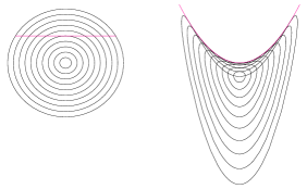
Figure 2. The basic example: the mapping $F(x,y)=(x,x^{2}-y^{2})$

Section 6 is mainly devoted to a new proof of Theorem 1.2. It will be obtained through an adaptation of an explicit example, which can be traced back at least to J.C. Wood [23], namely, the polynomial harmonic mapping $F(x,y)=(x,x^{2}-y^{2})$. It is easily seen that such a mapping has a non–convex range. It shows also that, contrary to what happens for holomorphic functions, a harmonic mapping may fail to be open, see Figure 2 on page 2. From our construction, we also obtain that, in Theorem 1.2, the boundary mapping $\Phi$ can be chosen in such a way that there exists a curve $\eta\subset B$ on which $\det DU$ vanishes and such that $U$ changes its orientation across $\eta$. In Remark 6.1 we also use this construction to show the considerable tightness of the condition of local homeomorphism at the boundary appearing in Theorem 1.7.

In the final Section 7, we first review the shear construction method of Clunie and Sheil–Small. Then we state and prove our improved version, namely Theorem 7.3. We conclude with Corollary 7.4 which provides a general construction of harmonic univalent mappings with prescribed dilatation.

2. Classical foundations

In what follows we shall identify, as usual, points $(x,y)\in\mathbb{R}^{2}$ with complex numbers $z=x+iy\in\mathbb{C}$. When needed, we shall use also polar coordinates $z=re^{i\theta}$.

We now recall some classical fundamental Theorems which we shall use several times in the paper.

Theorem 2.1 (Monodromy).

Let $U\in C(\overline{B};\mathbb{R}^{2})$ be such that

a) $\Phi=U\big{|}_{\partial B}$ is a homeomorphism of $\partial B$ onto a simple closed curve $\gamma$.

b) For every $P\in\overline{B}$, $U$ is a local homeomorphism at $P$.

Then $U$ is a global homeomorphism of $\overline{B}$ onto $\overline{D}$, where $D$ is the bounded domain such that $\partial D=\gamma$.

Proof.

A proof can be found in [21, p.175]. Another proof might also be obtained via the theory of light and open mappings of Stoilow [20]. Results of the same nature in any dimension, but of higher sophistication, are due to Meisters and Olech [14] and Weinstein [22]. ∎

A variant that we shall also use is the following.

Theorem 2.2.

Let $U\in C^{1}(\overline{B};\mathbb{R}^{2})$ be such that

a^′) $\Phi=U\big{|}_{\partial B}$ is a sense preserving $C^{1}$ diffeomorphism of $\partial B$ onto a simple closed curve $\gamma$.

b^′) $\det DU(P)>0$, for every $P\in\overline{B}$.

Then $U$ is a global diffeomorphism of $\overline{B}$ onto $\overline{D}$.

Proof.

A proof can be readily obtained as a consequence of Theorem 2.1. ∎

Of a different character is the following Theorem due to H. Lewy ensuring that harmonic homeomorphisms are, in fact, diffeomorphisms as in the holomorphic case.

Theorem 2.3 (H. Lewy).

Let $U:B\to\mathbb{R}^{2}$ be harmonic. If $U$ is a sense preserving homeomorphism, then

$$\det DU>0\quad\hbox{everywhere in $B$.}$$

Proof.

We refer to [13] for a proof. ∎

3. Preliminary results

Here we collect some (new) results of essentially topological nature regarding harmonic functions and harmonic mappings.

Definition 3.1.

Given a nonconstant harmonic function $u$ defined in $B$, we denote by $M$ the sum of the multiplicities of its critical points. Hence $M$ is either a nonnegative integer or $+\infty$. Given $U=(u,v):B\to\mathbb{R}^{2}$ harmonic, we set, for every $\alpha\in[0,2\pi]$

(3.1) $$u_{\alpha}=\cos(\alpha)u+\sin(\alpha)v$$

and denote by $M_{\alpha}$ the sum of the multiplicities of the critical points of $u_{\alpha}$. Our convention is that $M:=M_{0}$.

Proposition 3.2.

Let $U\in C^{1}(\overline{B};\mathbb{R}^{2})$ be harmonic in $B$. If $\det DU>0$ on $\partial B$, then for every $\alpha\in[0,2\pi]$, the number $M_{\alpha}$ is finite and we have $M_{\alpha}=M$ for every $\alpha\in[0,2\pi]$.

Corollary 3.3.

Let $U$ be as in Proposition 3.2. We have $\det DU>0$ everywhere in $B$ if and only if there exists $\alpha\in[0,2\pi]$, such that $\nabla u_{\alpha}\neq 0$ everywhere in $B$.

Proof of Proposition 3.2.

Obviously $\nabla u_{\alpha}\neq 0$ everywhere on $\partial B$ for every $\alpha\in[0,2\pi]$. By the argument principle for holomorphic functions

$$M_{\alpha}=\frac{1}{2\pi}\int_{\partial B}\textrm{d}~{}{\rm arg}(\nabla u_{\alpha})\,,\quad\hbox{for every $\alpha\in[0,2\pi]$.}$$

We shall show that $M_{\alpha}=M_{0}$ for every $\alpha\in[0,2\pi]$. It is clear that it suffices to consider $\alpha\in\left(0,\pi\right)$. We set

$$J=\left(\begin{array}[]{cc}0&-1\\ 1&0\end{array}\right)$$

and we have

$$\nabla u_{\alpha}\cdot J\nabla u=\sin(\alpha)\det DU>0,\quad\hbox{on $\partial B$,}$$

hence $|{\rm arg}(\nabla u_{\alpha})-{\rm arg}(J\nabla u)|<\pi$. We conclude that

$$M_{\alpha}=\frac{1}{2\pi}\int_{\partial B}{\rm d\,arg}(\nabla u_{\alpha})=\frac{1}{2\pi}\int_{\partial B}{\rm d\,arg}(J\nabla u)=M_{0}.$$

∎

Proof of Corollary 3.3.

Let us assume that for a given $\alpha\in[0,2\pi]$, we have $M_{\alpha}=0$. By Proposition 3.2 one has $M_{\alpha}=0$ for every $\alpha\in[0,2\pi]$. Hence, for every $P\in B$, the vectors $\nabla u(P)$ and $\nabla v(P)$ are linearly independent, that is $\det DU(P)\neq 0$. Being $\det DU>0$ on $\partial B$, by continuity we have $\det DU>0$ everywhere in $B$. The reverse implication is trivial.∎

Definition 3.4.

Given a closed curve $\gamma$, parameterized by $\Phi\in C^{1}(\partial B;\mathbb{R}^{2})$ and such that

$$\frac{\partial\Phi}{\partial\theta}\neq 0,\ \textrm{for every}\ \theta\in[0,2\pi],$$

we define the winding number of $\gamma$ as the following integer

$${\rm WN}(\gamma)=\frac{1}{2\pi}\int_{\partial B}{\rm d\,arg}\left(\frac{\partial\Phi}{\partial\theta}\right).$$

Definition 3.5.

Let $u$ be a harmonic function in $B$. We denote by $\tilde{u}$ its conjugate harmonic function and we set

$$f=u+i\tilde{u}.$$

Note that if, in addition, $u\in C^{1}(\overline{B})$ and $\nabla u\neq 0$ on $\partial B$, then $f\big{|}_{\partial B}$ gives us a regular $C^{1}$ parametrization of a closed curve.

Proposition 3.6.

Let $u\in C^{1}(\overline{B})$ be harmonic in $B$. If $\nabla u\neq 0$ on $\partial B$, then

$$M={\rm WN}(f(\partial B))-1,$$

with $M$ as in Definition 3.1.

Proof.

The proof is elementary, and we claim no novelty in this case. We have

$${\rm WN}(f(\partial B))=\frac{1}{2\pi}\int_{\partial B}{\rm d\,arg}\left(\frac{\partial f}{\partial z}\frac{\partial z}{\partial\theta}\right)=\frac{1}{2\pi}\int_{\partial B}\textrm{d}~{}\left[{\rm arg}\left(\frac{\partial f}{\partial z}\right)+\theta\right]=$$

$$\frac{1}{2\pi}\int_{\partial B}\textrm{d}~{}{\rm arg}(\nabla u)+1=M+1.$$

∎

Remark 3.7.

If $U=(u,v)\in C^{1}(\overline{B};\mathbb{R}^{2})$ is such that $\det DU>0$ on $\partial B$, then, for any $P\in\partial B$, the mapping $U$ is a diffeomorphism near $P$. Hence, on $\partial B$, partial derivatives with respect to $u$ and $v$ make sense.

Lemma 3.8.

Let $U=(u,v)\in C^{1}(\overline{B};\mathbb{R}^{2})$ be harmonic in $B$. If

$$\det DU>0,\qquad{\rm on}\qquad\partial B,$$

then

$$\frac{\partial\tilde{u}}{\partial v}>0,\qquad{\rm on}\qquad\partial B,$$

where $\tilde{u}$ is the harmonic conjugate of $u$.

Proof.

We compute

$$\frac{\partial\tilde{u}}{\partial v}=\frac{\partial\tilde{u}}{\partial x}\frac{\partial x}{\partial v}+\frac{\partial\tilde{u}}{\partial y}\frac{\partial y}{\partial v}=\frac{1}{\det DU}\left(-\frac{\partial\tilde{u}}{\partial x}\frac{\partial u}{\partial y}+\frac{\partial\tilde{u}}{\partial y}\frac{\partial u}{\partial x}\right)=\frac{|\nabla u|^{2}}{\det DU}>0.$$

∎

We are now ready to state a Theorem which contains the main elements towards a proof of Theorem 1.3.

Theorem 3.9.

Let $U\in C^{1}(\overline{B};\mathbb{R}^{2})$ be harmonic in $B$ and let $\Phi=U\big{|}_{\partial B}$. If $\det DU>0$ on $\partial B$, then we have

(3.2) $${\rm WN}(f(\partial B))={\rm WN}(\Phi(\partial B)).$$

The proof of Theorem 3.9 will be based on the following two results.

Proposition 3.10.

Given a $C^{1}$ curve parameterized by $\Phi=(\phi,\psi):[a,b]\to\mathbb{R}^{2}$ and such that $\phi^{\prime}\neq 0$ in $(a,b)$ and $\phi^{\prime}(a)=\phi^{\prime}(b)=0$ and given a $C^{1}$ function $g:\psi([a,b])\to\mathbb{R}$ with $g^{\prime}>0$ in $\psi((a,b))$, consider the curve $\widetilde{\Phi}:[a,b]\to\mathbb{R}^{2}$ given by $\widetilde{\Phi}=(\phi,g(\psi))$. We have

(3.3) $$\int_{a}^{b}{\rm d\,arg}(\widetilde{\Phi}^{\prime})=\int_{a}^{b}{\rm d\,arg}(\Phi^{\prime}).$$

Lemma 3.11.

Under the same assumptions of Theorem 3.9, assuming in addition that $\frac{\partial u}{\partial\theta}\Big{|}_{\partial B}$ vanishes at finitely many points, we have that (3.2) holds.

Proof of Proposition 3.10.

Without loss of generality we may assume $\phi^{\prime}>0$ in $(a,b)$. We have that both ${\rm arg}\big{(}\Phi^{\prime}\big{)}$ and ${\rm arg}\big{(}\widetilde{\Phi}^{\prime}\big{)}$ take values in $(-\pi,\pi)$. Hence

$$\int_{a}^{b}{\rm d\,arg}(\Phi^{\prime})={\rm arg}\big{(}\Phi^{\prime}(b^{-})\big{)}-{\rm arg}\big{(}\Phi^{\prime}(a^{+})\big{)}$$

and also

$$\int_{a}^{b}{\rm d\,arg}(\widetilde{\Phi}^{\prime})={\rm arg}\big{(}\widetilde{\Phi}^{\prime}(b^{-})\big{)}-{\rm arg}\big{(}\widetilde{\Phi}^{\prime}(a^{+})\big{)}.$$

Now, we compute

$${\rm arg}(\Phi^{\prime}(b^{-}))={\rm arg}(\widetilde{\Phi}^{\prime}(b^{-}))=\pm\frac{\pi}{2},$$

and also

$${\rm arg}(\Phi^{\prime}(a^{+}))={\rm arg}(\widetilde{\Phi}^{\prime}(a^{+}))=\pm\frac{\pi}{2}.$$

Hence (3.3) follows.∎

Proof of Lemma 3.11.

Up to a rotation in the $x,y$ coordinates, we may assume without loss of generality that there exists a partition of $[0,2\pi]$, $0=\theta_{0}<\theta_{1}<\ldots<\theta_{N}=2\pi$ such that

$$\frac{\partial\phi}{\partial\theta_{k}}(\theta)=0\quad\hbox{for all}\quad k=0,1,\ldots,N-1,$$

and

$$\frac{\partial\phi}{\partial\theta}(\theta)\neq 0\quad\hbox{in}\quad(\theta_{k},\theta_{k+1}),\quad\hbox{for every}\quad k=0,1,\ldots,N-1.$$

On each interval $[\theta_{k},\theta_{k+1}]$, we have

$$f(e^{i\theta})=\Big{(}\phi(\theta),g(\psi(\theta))\Big{)}\quad\hbox{with}\quad g\big{(}\psi(\theta)\big{)}=\tilde{u}(e^{i\theta})$$

and, by Lemma 3.8,

$$\frac{\partial g}{\partial\psi}=\frac{\partial\tilde{u}}{\partial v}>0.$$

Hence, by Proposition 3.10

$$\int_{\theta_{k}}^{\theta_{k+1}}{\rm d\,arg}\left(\frac{\partial f}{\partial\theta}\right)=\int_{\theta_{k}}^{\theta_{k+1}}{\rm d\,arg}\left(\frac{\partial\Phi}{\partial\theta}\right)\quad\hbox{for every}\quad k=0,1,\ldots,N-1$$

and (3.2) follows.∎

Proof of Theorem 3.9.

By continuity, there exists $\rho\in(0,1)$, such that $\det DU>0$ in $\overline{B}\setminus B_{\rho}(0)$ and, consequently, $\frac{\partial f}{\partial z}\neq 0$ in $\overline{B}\setminus B_{\rho}(0)$. Therefore the numbers

$${\rm WN}\Big{(}f\big{(}\partial B_{r}(0)\big{)}\Big{)}\quad\hbox{and}\quad{\rm WN}\Big{(}U\big{(}\partial B_{r}(0)\big{)}\Big{)}$$

are constant with respect to $r\in[\rho,1]$. Since $u\big{|}_{\partial B_{r}}(\theta)$ is a nonconstant real analytic function of $\theta$, we have that $\frac{\partial u}{\partial r}\big{(}re^{i\theta}\big{)}$ vanishes at most on a finite set of angles $\theta_{j}\in[0,2\pi]$. Applying Lemma 3.11 to $U(r\cdot)$ rather than $U$, we obtain

$${\rm WN}\Big{(}f\big{(}\partial B\big{)}\Big{)}={\rm WN}\Big{(}f\big{(}\partial B_{r}(0)\big{)}\Big{)}={\rm WN}\Big{(}U\big{(}\partial B_{r}(0)\big{)}\Big{)}={\rm WN}\Big{(}\Phi\big{(}\partial B\big{)}\Big{)}.$$

∎

4. Proofs of the main Theorems

Proof of Theorem 1.3.

Let us assume that (1.2) holds. By assumption $\Phi$ is one–to–one and sense preserving. Hence by Theorem 3.9,

$${\rm WN}\Big{(}f\big{(}\partial B\big{)}\Big{)}={\rm WN}\Big{(}\Phi\big{(}\partial B\big{)}\Big{)}=1.$$

By Proposition 3.6, $\nabla u$ never vanishes in $B$. By Corollary 3.3, $\det DU>0$ everywhere in $\overline{B}$. By Theorem 2.2, $U:\overline{B}\to\overline{D}$ is a diffeomorphism. The reverse implication is obvious. ∎

Our next goal is to prove Theorem 1.7. We need the following preliminary Lemma.

Lemma 4.1.

Assume $\Phi:\partial B\to\gamma\subset\mathbb{R}^{2}$ is a homeomorphism onto a simple closed curve $\gamma$. Let $U\in C^{2}(B;\mathbb{R}^{2})\cap C(\overline{B};\mathbb{R}^{2})$ be the solution to (1.1). If, in addition, for every $P\in\partial B$ the mapping $U$ is a local homeomorphism near $P$, then there exists $\rho\in(0,1)$ such that $U$ is a diffeomorphism of $B\setminus\overline{B_{\rho}(0)}$ onto $U\Big{(}B\setminus\overline{B_{\rho}(0)}\Big{)}$.

Proof.

By the compactness of $B$, there exist finitely many points $P_{1},\ldots,P_{k}\in\partial B$ and a number $\delta>0$ such that

$$\partial B\subset\bigcup\limits_{k=1}^{K}B_{\delta}(P_{k}),$$

and $U$ is one–to–one on $B_{2\delta}(P_{k})\cap\overline{B}$ for every $k$. Note that there exists $\rho\in(0,1)$ such that

$$\overline{B}\setminus B_{\rho}(0)\subset\bigcup\limits_{k=1}^{K}B_{\delta}(P_{k}).$$

Let $P,Q$ be two distinct points in $\overline{B}\setminus B_{\rho}(0)$. If $|P-Q|<\delta$, then there exists $k=1,\ldots,K$ such that $P,Q\in B_{2\delta}(P_{k})$ and, hence, $U(P)\neq U(Q)$. Assume now $|P-Q|\geq\delta$. Let

$$P^{\prime}=\frac{P}{|P|}\quad,\quad Q^{\prime}=\frac{Q}{|Q|}.$$

We have $|P-P^{\prime}|<1-\rho,\,|Q-Q^{\prime}|<1-\rho,$ and thus

$$|P^{\prime}-Q^{\prime}|>|P-Q|-2(1-\rho)\geq\delta-2(1-\rho).$$

Choosing $\rho$ such that $(1-\rho)<\frac{\delta}{4}$, we have $|P^{\prime}-Q^{\prime}|>\frac{\delta}{2}.$ Now we use the fact that $P^{\prime}$ and $Q^{\prime}$ belong to $\partial B$ and $\Phi$ is one–to–one to deduce that there exists $c>0$ such that

$$|\Phi(P^{\prime})-\Phi(Q^{\prime})|\geq c.$$

Recall that $U$ is uniformly continuous on $\overline{B}$. Denoting by $\omega$ its modulus of continuity, we have

$$|U(P)-U(Q)|\geq|U(P^{\prime})-U(Q^{\prime})|-2\omega(1-\rho)=$$

$$|\Phi(P^{\prime})-\Phi(Q^{\prime})|-2\omega(1-\rho)\geq c-2\omega(1-\rho).$$

Choosing $\rho$ such that $1-\rho<\omega^{-1}\big{(}\frac{c}{4}\big{)}$ we obtain

$$|U(P)-U(Q)|\geq\frac{c}{2}>0,$$

which implies the injectivity of $U$ in $\overline{B}\setminus B_{\rho}(0)$. Consequently, by Theorem 2.3, $\det DU\neq 0$ in $B\setminus\overline{B_{\rho}(0)}$ and the thesis follows. ∎

Proof of Theorem 1.7.

We assume that, for every $P\in\partial B$, $U$ is a local homeomorphism near $P$ and prove that $U:\overline{B}\to\overline{D}$ is a homeomorphism. The opposite implication is trivial. In view of Theorem 2.1 it suffices to show that $\det DU\neq 0$ everywhere in $B$.

For every $r\in(0,1)$, let us write $\Phi^{r}:\partial B\to\mathbb{R}^{2}$ to denote the application given by

$$\Phi^{r}(e^{i\theta})=U(re^{i\theta}),\quad\theta\in[0,2\pi].$$

By Lemma 4.1, there exists $\rho\in(0,1)$ such that for every $r\in(\rho,1)$ the mapping $\Phi^{r}:\partial B\to\gamma_{r}\subset\mathbb{R}^{2}$ is a diffeomorphism of $\partial B$ onto a simple closed curve $\gamma_{r}$, and $U(r\cdot)\in C^{1}(\overline{B};\mathbb{R}^{2})$ solves (1.1) with $\Phi$ replaced by $\Phi^{r}$. Then, by Theorem 1.3 we obtain

$$\det DU(rz)\neq 0,\quad\hbox{for every}\quad z\in\overline{B}$$

that is

$$\det DU(z)\neq 0,\quad\hbox{for every}\quad z\in\overline{B_{r}(0)}.$$

Finally, by Lemma 4.1 we have $\det DU\neq 0$ in $B\setminus\overline{B_{\rho}(0)}$ so that $\det DU\neq 0$ everywhere in $B$. ∎

5. Variations upon Theorem 1.3

Let us introduce some definitions borrowed from the literature on minimal surfaces [18].

Definition 5.1.

Given a Jordan domain $D$, let us denote by ${\rm co}(D)$ its convex hull. We define the convex part of $\partial D$ as the closed set $\gamma_{c}=\partial D\cap\partial({\rm co}(D))$. Consequently we define the non–convex part of $\partial D$ as the open set $\gamma_{nc}=\partial D\setminus\partial({\rm co}(D))$.

Theorem 5.2.

Under the same assumptions as in Theorem 1.3, the mapping $U$ is a diffeomorphism of $\overline{B}$ onto $\overline{D}$ if and only if

(5.1) $$\det DU>0\quad\hbox{everywhere on $\Phi^{-1}(\gamma_{nc})$},$$

where $\gamma_{nc}$ is the set introduced in Definition 5.1 above.

First we prove the following Lemma.

Lemma 5.3.

Under the assumptions of Theorem 1.3, we always have

(5.2) $$\det DU>0\quad\hbox{everywhere on $\Phi^{-1}(\gamma_{c})$}.$$

Proof.

Let $P\in\Phi^{-1}(\gamma_{c})$ and $Q=\Phi(P)$. Let $l$ be a support line for ${\rm co}(D)$ at $Q$. Without loss of generality, we may assume

$$\begin{array}[]{lll}l=\{(u,v)\in\mathbb{R}^{2}:v=0\}&,&{\rm co}(D)\subset\{(u,v)\in\mathbb{R}^{2}:v>0\}.\end{array}$$

Thus the second component $\psi$ of $\Phi$ satisfies

$$\psi\geq 0\quad\hbox{everywhere},\quad\psi(P)=0,$$

hence $P$ is a minimum point for $\psi$ and therefore

$$\frac{\partial\psi}{\partial\theta}(P)=0.$$

Moreover, being $\Phi$ orientation preserving, we have that $\phi$ is increasing at $P$ and also

$$\left(\frac{\partial\phi}{\partial\theta}(P)\right)^{2}=\left|\frac{\partial\Phi}{\partial\theta}(P)\right|^{2}>0$$

so that

$$\frac{\partial\phi}{\partial\theta}(P)>0.$$

On the other hand, Hopf’s Lemma gives

$$\frac{\partial v}{\partial r}(P)<0.$$

Consequently

$$\det DU(P)=-\frac{\partial\phi}{\partial\theta}(P)\frac{\partial v}{\partial r}(P)>0.$$

∎

Proof of Theorem 5.2.

The proof is a straightforward consequence of Theorem 1.3 and of the above Lemma 5.3. ∎

We now turn to the Hilbert transform formalism. For any $g\in L^{2}((0,2\pi))$, let

(5.3) $$\mathcal{H}g(\theta):=\frac{1}{2\pi}\ {\rm P.V.}\!\!\!\int_{0}^{2\pi}\frac{g(\tau)}{{\rm tan}\left(\frac{\theta-\tau}{2}\right)}d\tau,\qquad\theta\in[0,2\pi],$$

be the Hilbert transform on the unit circle, see for instance [19, p. 145]. The following is an equivalent formulation of Theorem 5.2 and thus of Theorem 1.3.

Theorem 5.4.

Under the same assumptions as in Theorem 1.3, $U$ is a diffeomorphism of $\overline{B}$ onto $\overline{D}$ if and only if the components $\phi$ and $\psi$ of $\Phi$ satisfy

(5.4) $$\frac{\partial\phi}{\partial\theta}\mathcal{H}\left(\frac{\partial\psi}{\partial\theta}\right)-\frac{\partial\psi}{\partial\theta}\mathcal{H}\left(\frac{\partial\phi}{\partial\theta}\right)>0\quad\hbox{everywhere on $\Phi^{-1}(\gamma_{nc})$.}$$

Proof.

Expressing $\det DU$ in polar coordinates we have, on $\partial B$,

$$\det DU=\frac{\partial u}{\partial r}\frac{\partial v}{\partial\theta}-\frac{\partial u}{\partial\theta}\frac{\partial v}{\partial r}.$$

Since $\frac{1}{r}\frac{\partial u}{\partial\theta}$ is the harmonic conjugate of $\frac{\partial u}{\partial r}$, we have that

(5.5) $$\frac{\partial u}{\partial r}=-\mathcal{H}\left(\frac{\partial u}{\partial\theta}\right)\quad\hbox{everywhere on $\partial B$}$$

and the same formula, obviously applies for $v$. By assumption $u,v\in C^{1}(\overline{B})$, hence we obtain

$$\det DU=\frac{\partial\phi}{\partial\theta}\mathcal{H}\left(\frac{\partial\psi}{\partial\theta}\right)-\frac{\partial\psi}{\partial\theta}\mathcal{H}\left(\frac{\partial\phi}{\partial\theta}\right)\quad\hbox{everywhere on $\partial B$}.$$

Hence condition (5.1) is equivalent to (5.4). ∎

6. The counterexample

Proof of Theorem 1.2.

It suffices to prove the Theorem with $D$ replaced by $TD$ where $T$ is an invertible affine transformation. In fact, the Theorem will be proved with $\Phi$ and $U$ replaced by $T^{-1}\Phi$ and $T^{-1}U$ respectively.

If $D$ is not convex, we can find a support line $l$ of its convex hull ${\rm co}(D)$ which touches $\partial D$ on (at least) two points $A$ and $B$ and such that the open segment $\overline{AB}$ is outside $\overline{D}$. The midpoint $C$ of $\overline{AB}$ is at a positive distance from $\overline{D}$. We can also find $E\in{\rm co}(D)\setminus D$ such that the segment $\overline{CE}$ is perpendicular to $\overline{AB}$ and it lies outside $\overline{D}$.

Next we consider $K$, the largest closed cone, with vertex at $E$, such that $K\cap D=\emptyset$. Note that $K\subseteq K^{\prime}$, where $K^{\prime}$ is the convex cone with vertex at $E$ and such that $A,B\in\partial K^{\prime}$. Therefore the cone $K$ is convex. Let $\alpha,\beta$ be the half–lines such that $\alpha\cup\beta=\partial K$. Then $\alpha$ intersects $\partial D$ in at least one point $A^{\prime}$ and similarly $\beta$ intersects $\partial D$ in at least one point $B^{\prime}$. Up to an affine transformation, we may assume that $|A^{\prime}-E|=|B^{\prime}-E|$.

Let ${\mathcal{P}}$ be the unique parabola contained in $K$ which passes through $A^{\prime}$ and $B^{\prime}$. Up to a further affine transformation, we may assume

$${\mathcal{P}}=\{(u,v)\big{|}v=u^{2}\},\quad A^{\prime}=(p,p^{2}),\quad B^{\prime}=(-p,p^{2})\quad\hbox{for some}\quad p>0.$$

Consider the harmonic mapping $F:\mathbb{R}^{2}\to\mathbb{R}^{2}$ given by

$$F(x,y)=(x,x^{2}-y^{2}).$$

Set

$$Y_{+}=\{y\geq 0\},\quad Y_{-}=\{y\leq 0\}\quad\hbox{and}\quad V_{-}=\{(u,v)\in\mathbb{R}^{2}\big{|}v\leq u^{2}\}.$$

The mappings $F_{\pm}=F\Big{|}_{Y_{\pm}}:Y_{\pm}\to V^{-}$ are both one–to–one.

Let $\gamma_{1},\gamma_{2}$ be the simple open arcs of $\gamma=\partial D$ whose endpoints are $A^{\prime}$ and $B^{\prime}$. Consider the closed curve $\Gamma$ obtained by gluing together the arcs

$$\Gamma_{1}=F^{-1}_{+}(\gamma_{1}),\quad\Gamma_{2}=F^{-1}_{-}(\gamma_{2}),$$

through their common endpoints $F^{-1}(A^{\prime})$ and $F^{-1}(B^{\prime})$. Then $\Gamma$ is a simple closed curve which intersects the line $\{y=0\}$ exactly at the two points, $F^{-1}(A^{\prime})=(p,0)$ and $F^{-1}(B^{\prime})=(-p,0)$. Let $G$ be the Jordan domain bounded by $\Gamma$ and let $\omega$ be a conformal mapping $\omega:B\to G$ which extends to a homeomorphism of $\overline{B}$ onto $\overline{G}$. We define

(6.1) $$\Phi=(F\circ\omega)\big{|}_{\partial B},\quad\hbox{and}\quad U=F\circ\omega,\quad\hbox{in}\quad B.$$

One then verifies that $\Phi:\partial B\to\partial D$ is a homeomorphism, that $U$ solves (1.1) and that it is not one–to–one. In fact, $\det DU$ changes its sign across the curve

$$\eta=\omega^{-1}\Big{(}\big{\{}(x,0)\in\mathbb{R}^{2}:|x|<p\big{\}}\Big{)}.$$

Moreover, $\det DU=0$ in $B$ if and only if $(x,y)\in\eta$ and $U$ maps the curve $\eta$ in a one–to–one way onto the arc of the parabola ${\mathcal{P}}$ which joins $A^{\prime}$ to $B^{\prime}$ and which lies outside $\overline{D}$. ∎

Figure 1. A sketch of the construction of the counterexample

Remark 6.1.

In the construction of our counterexample the harmonic mapping $U$ given by (6.1) fails to be a local homeomorphism on $\partial B$ exactly at the points $A^{\prime\prime}=\omega^{-1}(p,0)$, $B^{\prime\prime}=\omega^{-1}(-p,0)$. This is a clear indication of how close to optimal Theorem 1.7 is. In fact, the conclusion of Theorem 1.7 does not hold if the condition

for every $P\in\partial B$, the mapping $U$ is a local homeomorphism at $P$

is relaxed to

for every $P\in\partial B$, except possibly at two points, the mapping $U$ is a local homeomorphism at $P$.

7. The shear construction revisited

Let us recall the so–called shear construction method due to Clunie and Sheil-Small [8]. In order to conform to the language of the previous sections, we shall adapt their definitions to the current notation of this paper.

Let $U=(u,v)$ be a harmonic mapping on $B$ and let $\tilde{u}$ and $\tilde{v}$ be the harmonic conjugates of $u$ and $v$ respectively. We already introduced the holomorphic function

(7.1) $$f=u+i\tilde{u}\ ,$$

accordingly, we define

(7.2) $$g=v+i\tilde{v}\ .$$

Let us further introduce the following linear combinations

(7.3) $$G=\frac{1}{2}\left(f+ig\right)\ ,\ H=\frac{1}{2}\left(f-ig\right).$$

Then we have

(7.4) $$U=G+\overline{H}$$

which is usually called the canonical representation of $U$. Note that, by construction, we have that $f$ as defined by (7.1), satisfies

(7.5) $$f=G+H\ .$$

Here with slight, although customary, abuse of notation we have identified $U=(u,v)$ with $u+iv$.

Definition 7.1.

For any $\theta\in[0,\pi)$, a set $K\subseteq\mathbb{R}^{2}$ is called convex in the direction $\zeta=e^{i\theta}$, if any line parallel to $\zeta$ intersects $K$ in a connected set, possibly empty or unbounded. We denote by $C_{\theta}$ the class of such sets. In particular, $C_{\pi/2}$ denotes the class of sets which are convex in the vertical direction and we write $f(B)\in C_{\theta}$ to indicate that the range of $f$ is convex in the direction $e^{i\theta}$.

The basic Theorem of the shear construction method is as follows.

Theorem 7.2 (Clunie and Sheil-Small).

Let $U$ be a harmonic mapping on $B$ with canonical representation as in (7.4), let $f$ be defined by (7.5) and assume that

(7.6) $$\det DU>0\,\,\mbox{in}\,\,B\ .$$

The following two conditions are equivalent

(7.7) $$U\text{ is one--to--one and }U(B)\in C_{\pi/2}\ ,$$

(7.8) $$f\text{ is one--to--one and }f(B)\in C_{\pi/2}\ .$$

A slightly more involved version of this result is available, which applies when the class of sets convex in one direction is replaced with the class of close–to-convex sets, we refer to [8, 6] for the definition and details. Our new version is the following.

Theorem 7.3.

Let $U\in C^{2}(B;\mathbb{R}^{2})\cap C^{1}(\overline{B};\mathbb{R}^{2})$ be harmonic on $B$ with canonical representation as in (7.4), let $f$ be defined by (7.5) and assume that

(7.9) $$\det DU>0\,\,\mbox{on}\,\,\partial B\ ,$$

then the following conditions are equivalent

(7.10) $$U\big{|}_{\partial B}\text{ is one--to--one }\ ,$$

(7.11) $$f\big{|}_{\partial B}\text{ is one--to--one }\ ,$$

(7.12) $$U\text{ is one--to--one on }\overline{B}\ ,$$

(7.13) $$f\text{ is one--to--one on }\overline{B}\ .$$

Proof (sketch)..

By Theorem 1.3, (7.10) is equivalent to (7.12). Theorem 1.3 can also be used to show that (7.11) is equivalent to (7.13), however a more direct proof can be obtained by the use of the classical argument principle. From Theorem 3.9 we readily obtain that (7.10) is equivalent to (7.11). ∎

Observe that, in comparison to Theorem 7.2, at the minor price of assuming $C^{1}$ regularity up to the boundary for $U$, we have obtained the advantage that the condition of non–vanishing of the Jacobian is now required on the boundary only, and that we do not need anymore the assumption of convexity in some direction. We recall also that one of the main interest of Theorem 7.2 is that it allows to construct univalent harmonic functions with prescribed dilatation

(7.14) $$\omega=\frac{\overline{U_{\bar{z}}}}{U_{z}}\ .$$

We refer the reader to the monograph of P. Duren [9] for more details about the meaning of the dilatation of a harmonic mapping, also called second complex dilatation or analytic dilatation. For the present purposes it suffices to recall that $\omega$ is holomorphic and that, at any point, the condition $\det DU>0$ is equivalent to $|\omega|<1$. If we are given a univalent holomorphic function $f$ and a holomorphic function $\omega$ such that $|\omega|<1$ in $B$ and such that $f(B)\in C_{\pi/2}$, then one can construct a harmonic univalent function $U$ such that $U(B)\in C_{\pi/2}$ and which has the canonical representation $U=G+\overline{H}$ where $G$ and $H$ are determined by the linear system

(7.15) $$\left\{\begin{array}[]{lll}G_{z}+H_{z}&=&f_{z}\\ \omega G_{z}-H_{z}&=&0.\end{array}\right.$$

In this way one obtains a harmonic injective mapping with prescribed dilatation $\omega$. The name of shear construction is related to the mechanical concept of shear deformation. Indeed $U$ is obtained from $f$, by keeping one component fixed (in this case the real part) and by deforming the other (in this case the imaginary part). The fundamental drawback is that one cannot apply the method when no sort of convexity assumption on the range of $f$ is available. As a consequence of our new Theorem 7.3 we can remove this kind of requirement.

Corollary 7.4.

Let $f,\omega$ be holomorphic functions in $B$ such that $f$ extends to a $C^{1}$ invertible mapping on $\overline{B}$, $\omega$ extends continuously to $\overline{B}$ and it satisfies

$$|\omega|<1\ ,\text{ in }\overline{B}\ .$$

Then, given $G,H$ the holomorphic solutions to (7.15), the harmonic mapping $U=G+\overline{H}$ is a diffeomorphism on $\overline{B}$, it satisfies $\mathfrak{Re}U=\mathfrak{Re}f$ and its dilatation equals $\omega$ in $\overline{B}$.

Proof.

Straightforward consequence of Theorem 7.3. ∎

Remark 7.5.

It is evident that if we merely assume $f,\omega$ be holomorphic functions in $B$ such that $f$ is invertible on $B$ and $\omega$ satisfies

$$|\omega|<1\ ,\text{ in }B\ ,$$

then the same construction yields a harmonic mapping $U$ which is a diffeomorphism on the open disk $B$. In fact, similarly to what we did in the proof of Theorem 1.7, it suffices to apply Corollary 7.4 by shrinking the independent variable $z\in B$ to $rz\in B_{r}(0)$ for any $0<r<1$. It is also evident, indeed, that the above construction provides a complete characterization of harmonic diffeomorphisms. In fact, given a harmonic diffeomorphism $U$ either on $\overline{B}$, or on $B$, $f$ and $\omega$ are immediately obtained by (7.1), (7.14).

Acknowledgement.

The authors express their gratitude to G. F. Dell’Antonio for inspiring and fruitful conversations occurred while completing this paper.

References

- [1] G. Alessandrini and A. Diaz Valenzuela, Unique determination of multiple cracks by two measurements, SIAM J. Control Optim. 34 (1996), no. 3, 913–921.
- [2] G. Alessandrini and V. Nesi, Univalent -harmonic mappings, Arch. Ration. Mech. Anal. 158 (2001), no. 2, 155–171.
- [3] by same author, Univalent -harmonic mappings: applications to composites, ESAIM Control Optim. Calc. Var. 7 (2002), 379–406 (electronic).
- [4] K. Astala, T. Iwaniec, G. J. Martin, and J. Onninen, Extremal mappings of finite distortion, Proc. London Math. Soc. (3) 91 (2005), no. 3, 655–702.
- [5] P. Bauman, A. Marini, and V. Nesi, Univalent solutions of an elliptic system of partial differential equations arising in homogenization, Indiana Univ. Math. J. 50 (2001), no. 2, 747–757.
- [6] D. Bshouty and W. Hengartner, Univalent harmonic mappings in the plane, Handbook of complex analysis: geometric function theory. Vol. 2, Elsevier, Amsterdam, 2005, pp. 479–506.
- [7] G. Choquet, Sur un type de transformation analytique généralisant la représentation conforme et définie au moyen de fonctions harmoniques, Bull. Sci. Math. (2) 69 (1945), 156–165.
- [8] J. Clunie and T. Sheil-Small, Harmonic univalent functions, Ann. Acad. Sci. Fenn. Ser. A I Math. 9 (1984), 3–25.
- [9] P. Duren, Harmonic mappings in the plane, Cambridge Tracts in Mathematics, vol. 156, Cambridge University Press, Cambridge, 2004.
- [10] A. Friedman and M. Vogelius, Determining cracks by boundary measurements, Indiana Univ. Math. J. 38 (1989), no. 3, 527–556.
- [11] H. Kim and J. K. Seo, Unique determination of a collection of a finite number of cracks from two boundary measurements, SIAM J. Math. Anal. 27 (1996), no. 5, 1336–1340.
- [12] H. Kneser, Lösung der Aufgabe 41, Jber. Deutsch. Math.-Verein. 35 (1926), 123–124.
- [13] H. Lewy, On the non-vanishing of the Jacobian in certain one-to-one mappings, Bull. Am. Math. Soc. 42 (1936), 689–692.
- [14] G. H. Meisters and C. Olech, Locally one-to-one mappings and a classical theorem on schlicht functions, Duke Math. J. 30 (1963), 63–80.
- [15] B. P. Palka, An introduction to complex function theory, Undergraduate Texts in Mathematics, Springer-Verlag, New York, 1991.
- [16] T. Radó, Aufgabe 41, Jber. Deutsch. Math.-Verein. 35 (1926), 49.
- [17] by same author, On the problem of Plateau, Subharmonic functions, Reprint, Springer-Verlag, New York, 1971.
- [18] F. Sauvigny, Uniqueness of Plateau’s problem for certain contours with a one-to-one, nonconvex projection onto a plane, Geometric analysis and the calculus of variations, Int. Press, Cambridge, MA, 1996, pp. 297–314.
- [19] V. I. Smirnov, A course of higher mathematics. Vol. III. Part two. Complex variables. Special functions, Translated by D. E. Brown. Translation edited by I. N. Sneddon, Pergamon Press, Oxford, 1964.
- [20] S. Stoïlow, Leçons sur les principes topologiques de la théorie des fonctions analytiques. Deuxième édition, augmentée de notes sur les fonctions analytiques et leurs surfaces de Riemann, Gauthier-Villars, Paris, 1956.
- [21] B. von Kerékjártó, Vorlesungen über Topologie. I.: Flächentopologie, Die Grundlehren der mathematischen Wissenschaften. Bd. 8 , J. Springer, Berlin, 1923.
- [22] A. Weinstein, A global invertibility theorem for manifolds with boundary, Proc. Roy. Soc. Edinburgh Sect. A 99 (1985), no. 3-4, 283–284.
- [23] John C. Wood, Singularities of harmonic maps and applications of the Gauss-Bonnet formula, Amer. J. Math. 99 (1977), no. 6, 1329–1344.