A Mathematical Model for Voigt Poro-Visco-Plastic Deformation

Abstract

A mathematical model for poro-visco-plastic compaction and pressure solution in porous sediments has been formulated using the Voigt-type rheological constitutive relation as derived from experimental data. The governing equations reduce to a nonlinear hyperbolic heat conduction equation in the case of slow deformation where permeability is relatively high and the pore fluid pressure is nearly hydrostatic, while travelling wave exists in the opposite limit where over-pressuring occurs and the pore fluid pressure is almost quasi-lithostatic. Full numerical simulation using a finite element method agree well with the approximate analytical solutions.

Citation detail: X. S. Yang, A mathematical model for Voigt poro-visco-plastic deformation, Geophys. Res. Lett., 29(5), 10.1029/2001GL014014 (2002).

1 Introduction

Many physical properties such permeability, viscosity, Young’s modulus and thermal conductivity vary with porosity or fluid content in sedements and minerals. The porosity in turn depends on the deformation and compaction state and can be calculated from the compaction curves resulting from the proper compaction modelling [Audet and Fowler, 1992]. Furthmore, compaction is also related to overpressuring, mineral deposition, hydrocarbon generation and oil migration in reservoir. Thus the correct modelling of compaction is both of scientific importance as well as industrial interest. However, due to the nonlinear feature in the compaction process and difficulty in formulating the accurate and realistic rheological relationship in sediments and rocks, most of existing models use simplified rheology such as poroelastic, purely viscous or viscoelastic relations [Rutter, 1976; Wangen, 1992; Holzbercher, 1998; Revil, 1999; Yang,2000]. The rheological properties of realistic granular sediments are usually viscoelastic or viscoplastic as implied by experiments. Yang [2000] presents a viscoelastic model of Maxwell type and comparison of analytical solutions with the numerical simulations shows very good agreement. However, Revil’s [1999] work suggests that it maybe more appropriate to use a poro-visco-plastic model of Voigt type. We intend to do the analysis similar to Yang’s [2000] but using the Voigt-type consitutive relation as derived by Revil [1999].

Much of the work in this area has been reviewed by Rieke and Chilingarian [1974], Birchwood and Turcotte [1994] and later by Fowler and Yang[1999]. This paper aims at providing a new approach to compaction and pressure solution by using Revil’s visco-poro-plastic relation of Voigt type [Revil, 1999]. The nonlinear partial differential equations are then analysed by using asymptotic methods and the obtained analytical solutions are compared with numerical simulations. Although the present work mainly concerns the 1-D theorectical formulation and analytical solution procedure, however, we intend to provide a simplified and yet realistic framework for further research in this area and shows how compaction mechanism is related to rheological relationships and material properties of porous sediments, so that more realistic constitutive relationships can be formulated and analysed.

2 MATHEMATICAL MODEL

The fundamental model of compaction and pressure solution is essentially similar to the model of soil consolidation process. The solid sediments act as a compressible porous matrix, so mass conservation of pore fluid together with Darcy’s law leads to an equation of the general type. Based on earlier work by Audet and Fowler [1992], Revil[1999] and Yang[2000], we can write down the poro-visco-plastic compaction model of Voigt type. In the one-dimensional case, we have the following governing equations

$$\frac{\partial(1-\phi)}{\partial t}+\frac{\partial}{\partial z}[(1-\phi)u^{s}]=0,$$ (1)

$$\frac{\partial\phi}{\partial t}+\frac{\partial(\phi u^{l})}{\partial z}=0,$$ (2)

$$\phi(u^{l}-u^{s})=-\frac{k(\phi)}{\mu}[\frac{\partial p}{\partial z}+\rho_{l}g],$$ (3)

$$-G\frac{\partial p_{e}}{\partial z}-\frac{\partial p}{\partial z}-\rho g=0,\,\,\,\,\rho=\rho_{s}(1-\phi)+\rho_{l}\phi,$$ (4)

where $\phi$ is porosity. $u^{l}$ and $u^{s}$ are the velocities of fluid and solid matrix, respectively. $k$ and $\mu$ are the matrix permeability and the liquid viscosity, $\rho_{l}$ and $\rho_{s}$ are the densities of fluid and solid matrix, $p_{e}$ is the effective pressure, $p^{l}$ is the pore pressure, and $g$ is the gravitational acceleration. $G=1+4\eta_{0}/3\xi_{0}$ is a constant describing the material properties with $\eta_{0}$ and $\xi_{0}$ being the shear modulus and bulk viscosity [Bird et al, 1977]. The first two equations are the conservation of mass for the solid phase and liquid phase, respectively. The third equation is the Darcy’s law in 1-D form and the last equation is actually the force balance in a simplified form whose detailed derivation can be found in [Fowler and Yang, 1998]. Combining equation (3) and (4), we have

$$\phi(u^{l}-u^{s})=\frac{k(\phi)}{\mu}[-G\frac{\partial p_{e}}{\partial z}-(\rho_{s}-\rho_{l})(1-\phi)g],$$ (5)

In writing the above equations, we have used an upward coordinate $z$ originating from $z=0$, which corresponds to the bottom of the sedimentary column, so that the ocean floor $z=h(t)$ moves as compaction proceeds. We use such a coordinate system because it simplifies the analytical solution procedure and also in keeping with the similar lines of earlier work in this area [Audet and Fowler, 1992; Yang, 2000]. However, the conventional depth coordinate is simply $z-h(t)$, thus the transformation shall be straightforward once the basin thickness $h(t)$ is known. As we shall see in the later sections, we provide an explicit formula for $h(t)$ as a very good approximation.

In addition, a rheological compactional relationship derived from experimental data [Revil, 1999] is needed to complete this model in the form

$$p_{e}=-\xi\frac{\partial u^{s}}{\partial z}-E\int^{t}_{0}\frac{\partial u^{s}}{\partial z}dt,$$ (6)

where $E$ is the elastic modulus and $\xi$ is the viscosity modulus. There are essentially the same parameters as introduced by Revil [1999]. The first term of the right hand of the equation is the usual contribution by viscous plastic deformation, while the second term corresponds to the poro-elastic deformation.

3 Non-dimensionalization

To write the governing equations in dimensionless forms, typical length and time scales are required. For a typical sedimentation rate $\dot{m}_{s}$, the corresponding typical time scale is $d/\dot{m}_{s}$ where the typical length scale $d$ can be defined as

$$d=\{\frac{\xi\dot{m}_{s}G}{(\rho_{s}-\rho_{l})g}\}^{1/2},$$ (7)

so that the dimensionless pressure $p=Gp_{e}/(\rho_{s}-\rho_{l})gd=O(1)$. Meanwhile, we scale $z$ with $d$, $u^{s}$ with ${\dot{m}}_{s}$, time $t$ with $d/{\dot{m}}_{s}$, permeability $k$ with $k_{0}$. By writing $k(\phi)=k_{0}k^{*}$, $z=dz^{*}$, …, and dropping the asterisks, we thus have

$$-\frac{\partial\phi}{\partial t}+\frac{\partial}{\partial z}[(1-\phi)u^{s}]=0,$$ (8)

$$\frac{\partial\phi}{\partial t}+\frac{\partial(\phi u^{l})}{\partial z}=0,$$ (9)

$$\phi(u^{l}-u^{s})=\lambda k(\phi)[-\frac{\partial p}{\partial z}-(1-\phi)],$$ (10)

$$p=-\frac{\partial u^{s}}{\partial z}-\Xi\int^{t}_{0}\frac{\partial u^{s}}{\partial z}dt$$ (11)

where

$$\lambda=\frac{k_{0}(\rho_{s}-\rho_{l})g}{\mu{\dot{m}}_{s}},\,\,\,\,\Xi=\frac{EG}{(\rho_{s}-\rho_{l})gd}.$$ (12)

Adding (8) and (9) together and integrating from the bottom, we have

$$u^{s}=-\phi(u^{l}-u^{s}),$$ (13)

where $u=\phi(u^{l}-u^{s})$ is the Darcy flow velocity. Now, we have

$$\frac{\partial\phi}{\partial t}=\frac{\partial}{\partial z}[(1-\phi)u^{s}],$$ (14)

$$u^{s}=\lambda(\frac{\phi}{\phi_{0}})^{m}[-\frac{\partial p}{\partial z}-(1-\phi)].$$ (15)

$$p=-\frac{\partial u^{s}}{\partial z}-\Xi\int^{t}_{0}\frac{\partial u^{s}}{\partial z}dt,$$ (16)

where we have used the nonlinear constitutive relation for permeability $k(\phi)$ of typical form [Smith, 1971]

$$k(\phi)=(\frac{\phi}{\phi_{0}})^{m},$$ (17)

where $\phi_{0}$ is the initial depositional porosity. The exponent $m$ has a typical value of $3\sim 6$ for sands and sandstones.

The boundary conditions are

$$\frac{\partial p}{\partial z}-(1-\phi)=0\,\,\,\,({\rm or\,\,equivalently,}\,\,\,\,u^{s}=0),\,\,\,\,{\rm at}\,\,\,\,z=0,$$ (18)

$$\phi=\phi_{0},\,\,\,p=0,$$

$$\dot{h}=\dot{m}_{s}+\lambda(\frac{\phi}{\phi_{0}})^{m}[\frac{\partial p}{\partial z}-(1-\phi)]\,\,\,\,{\rm at}\,\,\,\,z=h(t).$$ (19)

It is useful to estimate these parameters by using values taken from observations. By using the typical values of $\rho_{l}\sim 10^{3}\,{\rm kg\,m}^{-3},\,\rho_{s}\sim 2.5\times 10^{3}\,{\rm kg\,m}^{-3},\,$ $k_{0}\sim 10^{-15}-10^{-20}\,{\rm m}^{2},\,\mu\sim 10^{-3}\,{\rm N\,s\,m}^{2},\,\xi\sim 1\times 10^{21}$ N s ${\rm m}^{-2},$ $\dot{m}_{s}\sim 300\,{\rm m\,\,Ma}^{-1}=1\times 10^{-11}\,{\rm m\,\,s}^{-1},\,g\sim 10{\rm m\,s}^{-2},\,E\sim 10^{9}{\rm N/m}^{2},\,G\sim 1,\,d\sim 1000{\rm m}$ ; then $\lambda\approx 0.01\sim 1000$ and $\Xi\sim 40$. We can see that the main parameters $\lambda$ and $\Xi$, which govern the evolution of the fluid flow and porosity in sedimentary basins, are the ratios of permeability to sedimentation rate and material modulus to the typical pressure scale. As $\lambda$ is essentially controlled by the hydraulic conductivity, so it becomes the dominant parameter controlling the whole compaction and pressure solution processes.

4 Asymptotic Analysis

Since the nondimensional parameter $\lambda\approx 0.01\sim 1000$ varies greatly and essentially controls the compaction process, we can expect that the two distinguished limits ($\lambda\ll 1$ and $\lambda\gg 1$) will have very different features in porosity and flow evolutions. In fact, $\lambda=1$ defines a transition between slow compaction ($\lambda\ll 1$) and fast compaction ($\lambda\gg 1$). The case of $\lambda\ll 1$ corresponds to the situation where the pore fluid pressure is nearly hydrostatic whereas the opposite case corresponds to an overpressured section in which the pore fluid pressure is quasi-lithostatic. Thus we can follow the similar asymptotic analysis [Fowler and Yang, 1998,1999] to obtain some analytical asymptotic solutions.

4.1 Slow Deformation ($\lambda\ll 1$)

In the nearly hydrostatic case of $\lambda\ll 1$, $z\sim 1$, $t\sim 1$, $p\sim 1$ implies that $u^{s}\ll 1$ and $\frac{\partial\phi}{\partial t}\approx 0$, then $\phi\approx\phi_{0}$. We thus have

$$\frac{\partial\phi}{\partial t}\approx-\lambda(1-\phi_{0})\frac{\partial^{2}p}{\partial z^{2}},$$ (20)

$$u^{s}\approx\lambda[-\frac{\partial p}{\partial z}-(1-\phi_{0})],$$ (21)

and using (20), we have

$$p\approx-\frac{\partial u^{s}}{\partial z}-\Xi\int^{t}_{0}\frac{1}{(1-\phi_{0})}\frac{\partial\phi}{\partial t}dt$$

$$=-\frac{1}{(1-\phi_{0})}(\frac{\partial\phi}{\partial t}+\Xi\phi),$$ (22)

combining these above three equations, we have a single equation for $\phi$

$$\frac{\partial\phi}{\partial t}=\lambda\Xi\frac{\partial^{2}\phi}{\partial z^{2}}+\lambda\frac{\partial^{3}\phi}{\partial t\partial z^{2}}.$$ (23)

As the $\Xi\gg 1$ and $\lambda\ll 1$, we can use the approximation $\phi_{t}\approx\lambda\Xi\phi_{zz}$ so that we have

$$\frac{\partial\phi}{\partial t}=\lambda\Xi\frac{\partial^{2}\phi}{\partial z^{2}}+\frac{1}{\Xi}\frac{\partial^{2}\phi}{\partial t^{2}}.$$ (24)

with appropriate boundary conditions

$$\frac{\partial\phi}{\partial z}\approx-\frac{(1-\phi_{0})^{2}}{\Xi},\,\,\,\,{\rm on}\,\,\,\,z=0,$$ (25)

$$\phi\rightarrow\phi_{0},\,\,\,\,z\rightarrow\infty,$$ (26)

This problem is in fact equivalent to the problem of hyperbolic heat conduction or non-Fourier heat equation which is well-documented in heat transfer and laser pulse modelling [Antaki, 1997]. By using the Laplace transform method, we can write the solution approximately in terms of Bessel functions $J_{i}$ as

$$\phi\approx(1-\phi_{0})\sqrt{4\lambda\Xi t}\,\,{\rm ierfc}(\zeta)$$

$$-\frac{(1-\phi_{0})^{2}}{\Xi}[\sqrt{\lambda\Xi t}+\frac{\lambda}{4\Xi}\sum_{i=1}^{\infty}\frac{J_{0}(z\alpha_{i})}{J_{0}(\alpha_{i})\alpha_{i}}],$$ (27)

where

$${\rm ierfc}(\zeta)=\frac{1}{\sqrt{\pi}}e^{-\zeta^{2}}-\zeta{\rm erfc}(\zeta).$$ (28)

and $\alpha_{i}$ is the ith real non-negative root of equation $J_{1}(\alpha_{i})=0$. We can see that compaction essentially occurs in a boundary layer near the bottom with a thickness of the order of $\sqrt{\lambda}$.

4.2 Fast Deformation ($\lambda\gg 1$)

In the case of $\lambda\gg 1$, the dependence of permeability on porosity $(\phi/\phi_{0})^{m}$ decrease dramatically, so that $\lambda(\phi/\phi_{0})^{m}$ is only bigger enough when $\phi>\phi_{*}=\phi_{0}\exp[-(\ln\lambda)/m]$. Thus, we have

$$\frac{\partial\phi}{\partial t}\approx(1-\phi_{*})\frac{\partial u^{s}}{\partial z},$$ (29)

$$\frac{\partial p}{\partial z}\approx(1-\phi),$$ (30)

and using the equation (29), we get

$$p=-\frac{1}{(1-\phi_{*})}\frac{\partial\phi}{\partial t}-\Xi\int^{t}_{0}\frac{1}{(1-\phi_{*})}\frac{\partial\phi}{\partial t}dt$$

$$=-\frac{1}{(1-\phi_{*})}(\frac{\partial\phi}{\partial t}+\Xi\phi).$$ (31)

Combining these equation, we can get a single equation for $\phi$

$$(1-\phi)(1-\phi_{*})=\frac{\partial^{2}\phi}{\partial t\partial z}+\Xi\frac{\partial\phi}{\partial z}.$$ (32)

Now we can seek the traveling wave solution of the form $\phi=\phi(\zeta)$ with $\zeta=z-ct$, so that we have

$$(1-\phi)(1-\phi_{*})=-c\phi^{\prime\prime}+\Xi\phi^{\prime}$$ (33)

where $\phi^{\prime}=d\phi/d\zeta$. We can easily write the solution as

$$\phi=1-(1-\phi_{0})\exp[\frac{[\Xi-\sqrt{\Xi+4c(1-\phi_{*})}]\zeta}{2c}]$$ (34)

In fact, the above solution is only valid for the top part when $\phi<\phi_{*}$. Using equation (6) and $\phi\sim\phi_{*}$ as $\zeta\rightarrow-\infty$, the travelling wave implies that

$$c\phi+(1-\phi)u^{s}=c\phi_{0}+(\dot{m}_{s}-c)(1-\phi_{0}).$$ (35)

so that we have

$$c\approx\dot{m}_{s}(\frac{1-\phi_{0}}{1-\phi_{*}}),\,\,\,\,h(t)\approx\dot{m}_{s}(\frac{1-\phi_{0}}{1-\phi_{*}}t,$$ (36)

which means the basin thickness increases linearly with time.

5 Numerical Simulations

In order to check the accuracy of the above analysis, we used a finite element method to solve the above equations (8)-(11). For simplicity, we only present the related results in Fig.1 where $t=5$ with different values of the $\lambda=0.001,0.1,10,1000$, $\phi_{0}=0.5$ and $\Xi=40$. This good agreement near the top and the bottom regions suggest that there exists a travelling wave solution on the top for $\lambda\gg 1$ and a boundary layer near the bottom for the small $\lambda$ case.

6 Discussion

A mathematical model for poro-visco-plastic comapction and pressure solution in porous sediments has been formulated using the Voigt-type rheological constitutive relation as derived from experimental data by Revil [1999]. After the proper scalings, the governing equations reduce to a system of coupled partial differential equations of mixed type. In the case of small $\lambda$ where the sedimentation is fast, permeability is small and the pore fluid pressure is nearly hydrostatic, the pressure solution process reduces to the case of hyperbolic heat conduction equation with a boundary layer forming at the bottom of the compacting column. On the other hand, for the large $\lambda\gg 1$ case where sedimentation or loading is slow in high permeable sediments, the travelling wave solution exists and the top surface moves up with nearly constant velocity.

Compared with the earlier work [Yang, 2000] using the viscoelastic rheological relation, we see that the there is no essential difference in the case small deformation ($\lambda\ll 1$). Boundary layer exists in both viscoelastic and poro-viscous-plastic cases although the slight difference is that the former viscoelastic case corresponds to the heat conduction with a constant flux and a constant source term, while the latter poro-visco-plastic case is mainly a hyperbolic heat condution mechanism. The case of fast deformation and compaction ($\lambda\gg 1$) is more complicated. Although both viscoelastic and poro-viscous-plastic cases have a transition at the depth where $\phi\approx\phi_{*}$, however, the mechanisms above and below the transition are very different. In the viscoelastic case, the top region is essentially poroelastic while the lower region is almost purely viscous, while in the present poro-visco-plastic case, the mechanism is a complicated combination of viscous-plastic mechanism and poro-elastic deformation process controlled by the proper balance of the parameters $\lambda$ and $\Xi$. Furthermore, in comparison with the earlier results, this work suggests that Voigt-type poro-visco-plastic deformation has much interesting characteristics due to its time-dependence feature.

Acknowledgments: The author would like to thank the referee(s) for their instructive and helpful comments which have greatly improved the original manuscript.

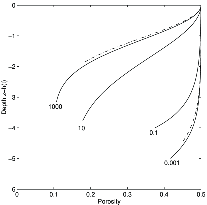
Figure 1: Comparison of numerical simulations (solid) with analytical solutions (dashed curves) for different values of $\lambda=0.001\sim 1000$ as marked on the curves.

References

- [1] Antaki, P J, 1997. Analysis of hyperbolic heat conduction in a semi-infinite slab with surface convection, Int. J. Heat Mass Trans., 40, 3247-3250.
- [2] Audet, D.M. & Fowler, A.C., 1992. A mathematical model for compaction in sedimentary basins, Geophys. J. Int., 110, 577-590.
- [3] Birchwood, R. A. & Turcotte, D. L., 1994. A unified approach to geopressuring, low-permeability zone formation, and secondary porosity generation in sedimentary basins, J. Geophys. Res., 99, 20051-20058.
- [4] Bird, R.B., Armstrong, R.C. & Hassager, O., 1977. Dynamics of polymeric liquids, Vol.1, John Wiley & Son press, New York.
- [5] Holzbercher, E. O., 1998. Modeling Density-Driven Flow in Porous Media: Principles, Numerics, Software. Springer-Verlag Berlin Heideberg, 286pp.
- [6] Fowler, A. C. and Yang, X. S., 1998. Fast and Slow Compaction in Sedimentary Basins, SIAM Jour. Appl. Math., 59, 365-385.
- [7] Fowler, A. C. and Yang, X. S., 1999. Pressure Solution and Viscous Compaction in Sedimentary Basins, J. Geophys. Res., B 104, 12 989-12 997.
- [8] Revil, A., 1999. Pervasive pressure solution transfer: a poro- visco-plastic model, Geophys. Res. Lett., 26, 255-258.
- [9] Rieke, H.H. & Chilingarian, C.V., 1974. Compaction of argillaceous sediments, Elsevier, Amsterdam, 474pp.
- [10] Rutter, E. H., 1976. The kinetics of rock deformation by pressure solution, Philos. Trans. R. Soc. London Ser.A 283, 203-219.
- [11] Smith, J.E., 1971. The dynamics of shale compaction and evolution in pore-fluid pressures, Math. Geol., 3, 239-263.
- [12] Wangen, M., 1992. Pressure and temperature evolution in sedimentary basins, Geophys. J. Int., 110, 601-613.
- [13] Yang, X. S., 2000. Nonlinear viscoelastic compaction in sedimentary basins, Nonlinear Proc. Geophysics, 7, 1-8.