Star formation in the outer Galaxy: membership and fundamental parameters of the young open cluster NGC 1893

Abstract

Context. Different environmental conditions can play a crucial role in determining final products of the star formation process and in this context, less favorable activities of star formation are expected in the external regions of our Galaxy.

Aims. We studied the properties of the young open cluster NGC 1893 located about 12 Kpc from the galactic center, to investigate how different physical conditions can affect the process of star formation.

Methods. By adopting a multiwavelength approach, we compiled a catalog extending from X-rays to NIR data to derive the cluster membership. In addition, optical and NIR photometric properties are used to evaluate the cluster parameters.

Results. We find 415 diskless candidate members plus 1061 young stellar objects with a circumstellar disk or class II candidate members, 125 of which are also H_α emitters. Considering the diskless candidate members, we find that the cluster distance is 3.6$\pm$0.2 kpc and the mean interstellar reddening is E(B-V)=0.6$\pm$0.1 with evidence of differential reddening in the whole surveyed region.

Conclusions. NGC 1893 contains a conspicuous population of pre-main sequence stars together with the well studied main sequence cluster population; we found a disk fraction of about 70% similar to that found in clusters of similar age in the solar neighbour and then, despite expected unfavorable conditions for star formation, we conclude that very rich young clusters can form also in the outer regions of our Galaxy.

1 Introduction

The sequence of events that characterize the star formation (SF) process starts from the compression of gas in a giant molecular cloud that produces molecular cores; these collapse into protostars evolving in pre-main sequence (PMS) objects through accretion of material and circumstellar disk formation (Zinnecker & Yorke, 2007). Within this standard picture, however, different environmental properties may play a key role by changing the physical conditions during the SF process and possibly the final products, for example the initial mass function (IMF).

SF regions with peculiar properties are therefore crucial for a complete understanding of the SF process since they are the natural places where different initial conditions can lead to the formation of clusters with non-standard IMF, dynamical evolution and/or disk fraction and evolution. In this context, clusters in the outer Galaxy are very interesting since they are located in regions where surface and volume densities of atomic and molecular hydrogen are much smaller than in the inner Galaxy (Wouterloot et al., 1990), while metal content is, on average, smaller (Wilson & Matteucci, 1992) and therefore higher temperatures of the cloud are expected due to lower radiative losses. In addition, the lack of prominent spiral arms and the presence of few supernovae as external triggers for SF are further indications of less likely SF conditions.

We have identified NGC 1893 as a very promising cluster for this kind of investigations since it is very young ($\sim$1-2 Myr), distant about 12 Kpc from the Galactic Center, with known massive members and indication of a large PMS population (Vallenari et al., 1999; Sharma et al., 2007). This SF region, located at the center of the Aur OB2 associations, is associated with the HII region IC 410 and the two pennant nebulae, Sim 19 and Sim 130 (Gaze & Shajn, 1952). It is obscured by several dust clouds and contains at least five O-type stars (Hiltner, 1966). The presence of several O-type stars and emission line B-type stars (Marco & Negueruela, 2002), likely in the PMS phase, is a strong indication that very recent SF events have occurred in this cluster.

Several photometric and low resolution spectroscopic works have been devoted to this cluster since the first study by Hoag et al. (1961). Many of them are, however, aimed at studying the NGC 1893 massive stars, that are in the MS phase (Becker & Fenkart, 1971; Moffat, 1972; Cuffey, 1973; Humphreys, 1978; Tapia et al., 1991; Fitzsimmons, 1993; Massey et al., 1995; Marco et al., 2001; Marco & Negueruela, 2002). Evidence of a large population of PMS stars in this cluster has been found by Vallenari et al. (1999) by using near-infrared photometry, even if their data did not allow them to distinguish the young population from the contaminating field stars. Only recently, Sharma et al. (2007) presented a study about the low mass population in NGC 1893 based on deep optical photometry down to V$\sim$22 and NIR 2MASS (Cutri et al., 2003) catalog. Several conclusions are drawn in this work about the IMF, the dynamical evolution and the effects of massive cluster stars on the low mass population. However, their results are based on a statistical subtraction of the field star population falling in the same region and suffer from the large statistical uncertainties related to the membership. In fact, the main challenge of the analysis of the low mass population in very young clusters is the membership derivation since PMS stars usually lie in the same region occupied by contaminating field stars and it is therefore crucial an accurate analysis to identify cluster members.

We have started a project aimed at the detailed study of the star formation process in NGC 1893 and in particular the unknown low mass population: the first results, based on the joint Chandra-Spitzer large program The Initial Mass Function in the Outer Galaxy: the star forming region NGC1893 (P.I. G. Micela), have been published in Caramazza et al. (2008, hereafter Paper I). In this latter paper, a conspicuous sample of low mass cluster members with circumstellar disk and of more evolved diskless candidate members belonging to this region has been identified by using Spitzer-IRAC and Chandra X-ray data.

We present here the results on the membership and cluster parameters based on a multiwavelength approach including new deep optical and JHK photometry that allow us to derive a more complete census of the low mass population in this cluster; knowledge of individual members is used to derive cluster parameters (reddening and distance) in a more accurate way than previously reported in the literature. Detailed studies on the X-ray coronal properties, disk fraction and evolution and IMF will be presented in forthcoming papers.

The present paper is organized as follow. In Sect. 2 we present the observations, the data reduction method and a description of the procedure used to derive the photometry and the astrometry. The whole catalog is presented in Sect. 3 while Sect. 4 includes the comparison with previous works; Sect. 5 describes how we identify cluster candidate members by using VRIJHK, H_α and X-rays data, while in Sect. 6 the cluster parameters are derived and a comparison with literature results is presented in Sect. 7. In Sect. 8 individual masses and ages are derived while in Sect. 9 we present our summary and conclusions.

2 Observations, data reduction and photometry

We present here new optical and near infrared (NIR) data of the cluster, collected from the Telescopio Nazionale Galileo (TNG) at the Roque de los Muchachos Observatory (ORM, Canary Islands, Spain), and from the 2.2 m telescope at the Calar Alto Observatory (Spain).

2.1 Optical data

Optical observations were acquired in service mode using two different telescopes, with the standard VRI and H$\alpha$ photometric filters: the Device Optimized for the LOw RESolution (DOLORES) mounted on the TNG was used in service mode during three nights in 2007, and the Calar Alto Faint Object Spectrograph (CAFOS), mounted on the 2.2 m telescope in Calar Alto German-Spanish Observatory (Spain), observed for three nights in 2007 and 2008, as detailed in Table 1. Standard fields were taken with both instruments to perform the required photometric calibration.

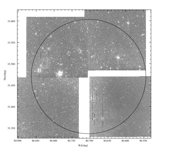
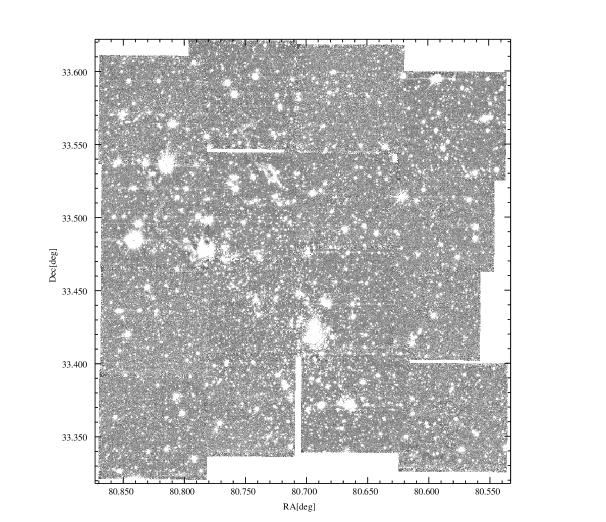
Figure 1: Upper panel: I band combined image of the four DOLORES frames of 740 sec; the overplotted circle indicates the CAFOS FoV. Bottom panel: Js band combined image of the NICS frames reduced and coadded with SNAP.

Table 1: Optical observations of the cluster NGC 1893

Date	$\alpha$ (J2000)	$\delta$ (J2000)	Instrument	Filter	Exp. time[sec]	seeing	airmass
2007/09/21	5:22:27.4	33:23:46.0	DOLORES	V	10, 60, $2\times 500$	1.0″	1.151–1.192
2007/09/21	5:22:27.5	33:23:36.9	DOLORES	R	10, 70, 700	1.0–1.1″	1.066–1.079
2007/09/21	5:22:27.4	33:23:42.5	DOLORES	I	10, 60, $2\times 740$	0.9″	1.095–1.138
2007/09/21	5:22:27.6	33:23:33.0	DOLORES	H$\alpha$	60, 300, $2\times 700$	0.9–1.0″	1.024–1.049
2007/10/18	5:23:11.6	33:23:34.3	DOLORES	V	10, 60, $2\times 500$	0.8″	1.026–1.040
2007/10/18	5:23:11.9	33:23:37.1	DOLORES	R	10, 70, 700	0.8–1.0″	1.006–1.010
2007/10/18	5:23:11.8	33:23:22.0	DOLORES	I	10, 60, $2\times 740$	0.8–1.0″	1.009–1.021
2007/10/18	5:23:12.8	33:23:47.2	DOLORES	H$\alpha$	60, 300, $2\times 700$	0.8″	1.013–1.031
2007/11/14	5:23:06.9	33:32:29.7	DOLORES	V	10, 60, $2\times 500$	1.0″	1.282–1.353
2007/11/14	5:23:06.8	33:32:14.6	DOLORES	R	10, 70, 700	1.0–1.1″	1.113–1.134
2007/11/14	5:23:06.7	33:32:24.5	DOLORES	I	10, 60, $2\times 740$	0.8–0.9″	1.184–1.257
2007/11/14	5:23:06.7	33:32:08.2	DOLORES	H$\alpha$	20, 60, 300, $2\times 700$	0.8″	1.050–1.096
2007/11/14	5:22:28.7	33:32:30.5	DOLORES	V	10, 60, $2\times 500$	1.0″	1.004–1.007
2007/11/14	5:22:33.9	33:32:39.3	DOLORES	R	$2\times 10$, 70, 700	0.8–0.9″	1.015–1.022
2007/11/14	5:22:32.0	33:32:20.5	DOLORES	I	10, 60, $2\times 740$	0.9–1.0″	1.004–1.010
2007/11/14	5:22:34.2	33:32:47.4	DOLORES	H$\alpha$	60, $2\times 300$, $2\times 700$	0.8″	1.029–1.066
2007/10/11	5:23:22.0	33:26:38.7	CAFOS	V	15, $3\times 500$	1.4–1.6″	1.002–1.004
2007/10/11	5:23:21.5	33:26:37.4	CAFOS	H$\alpha$	15, 100, $3\times 500$	1.6–1.8″	1.002–1.016
2008/01/05	5:23:23.3	33:26:42.4	CAFOS	V	10, 60, $2\times 300$	2.4″	1.161–1.205
2008/01/05	5:23:23.2	33:26:45.8	CAFOS	R	10, 60, $2\times 300$	2.3–2.6″	1.231–1.283
2008/01/05	5:23:23.3	33:26:47.3	CAFOS	I	10, 60, $3\times 500$	1.5–1.6″	1.353–1.502
2008/01/05	5:23:23.1	33:26:38.9	CAFOS	H$\alpha$	10, 60, 500	1.4″	1.603–1.651
2008/01/09	5:23:24.2	33:26:41.6	CAFOS	H$\alpha$	15, 100, $3\times 500$	1.2–1.7″	1.139–1.239

DOLORES is a focal reducer instrument equipped with a 2048$\times$2048 square pixels CCD, with a scale of 0.252^′′/px and a field of view (FoV) of 8.6′$\times$8.6′. A mosaic of four fields was made, covering an approximate area of 22.2′$\times$18.0′. The standard VRI filters were used in the four fields, as well as the H$\alpha$ narrow band filter centered on 6658 $\AA$, with a Full Width Half Maximum (FWHM) of 57 $\AA$. We also observed the standard field SA 98 (Landolt, 1992, $\alpha$=6^h:52^m:04.1^s, $\delta$=-00^d:19^m:37.9^s).

CAFOS is a focal reducer instrument that works with a CCD of 2048$\times$2048 square pixels, and has a scale of 0.53^′′/px, covering a circular FoV of 16′ diameter. With this FoV we covered the central areas of the cluster not observed by the four DOLORES fields. Standard VRI filters were used, together with an H$\alpha$ filter centered at 6577 $\AA$ with FWHM of 98 $\AA$. The fields used as standard for the photometric calibration were RU 149 ($\alpha$=07^h:24^m:40.8^s, $\delta$=-00^d:34^m:10.0^s), PG 2331 ($\alpha$=23^h:34^m:14.1^s, $\delta$=+05^d:46^m:25.9^s), and SA 95 ($\alpha$= 03^h:53^m:32.9^s, $\delta$=+00^d:00^m:48.3^s). In this case we noticed some variability in the photometric conditions of the last two nights in Calar Alto. To improve the quality of the photometric calibration we used also a set of local standards of the cluster, selected during the TNG data calibration, as explained below. A combined image of the four TNG fields in the I band, with the shape of the CAFOS FoV over plotted, is shown in Fig. 1.

Optical data were reduced using the standard Image Reduction and Analysis Facility (IRAF) routines, including the bias and flatfield subtraction. Bias correction was applied by using Zero images and the local overscan strip in each image. Some non-standard steps were taken due to various problems arisen during in the reduction, with details described below.

For the DOLORES observations a combination of sky flat-fields was used to create a master flat field in each band, using the task flatcombine. Once the images were corrected from flat-field, a strong illumination pattern was still present in the images of the I band. An illumination function was created using the flat-field (with the task mkillumflat), and conveniently removed from images. A pattern of interference fringing was still present in the I band images, with no variations found in the different nights. We constructed a fringing image by combining 15 images in the I band of the three nights, so the stars in the different fields are canceled. The images selected were of short exposure (2–60 s) to reduce the number of stars in the fields. The resulting fringing pattern was successfully corrected using the task mkfringecor and applied to every image in the I band.

For the CAFOS data, dome flats were used to correct the images from local irregularities. The singular circular shape of the FoV required special care: the values of all the pixels outside the FoV (easy to filter because they are well below the background) were set to a very large number; in this way no unreal features are created in the target images after subsequent flat-field removal, resulting in a value well below background outside the FoV. The remaining reduction followed the standard path.

2.2 NIR data

NIR observations were acquired in service mode at the TNG, using the large field Near Infrared Camera Spectrometer (NICS), that is a camera equipped with a 1024$\times$1024 square pixels HgCdTe HAWAII infrared array, with a scale of 0.25^′′/pix and a FoV of 4.2^′$\times$4.2^′(Baffa et al., 2001). Our observations were acquired with the Js(1.25 $\mu$), H(1.63 $\mu$) and K’(2.12 $\mu$) filters during eight nights in 2007 and 2008; we observed the whole field with a raster of 4$\times$4 pointings, at each pointing we obtained a series of NINT dithered exposures; each exposure is a repetition of a DIT (Detector Integration Time) times NDIT (number of DIT), to avoid saturation of the background; details are given in Table 2.

Table 2: Near Infrared observations of the cluster NGC 1893 from NICS; NINTs is the number of single frames.

Date	Field	$\alpha$ (J2000)	$\delta$ (J2000)	Filter	Exp. time[sec]	NINTs	seeing	airmass
2007/10/08	10	5:22:59.1	33:25:20.2	H	600	15	0.8″	1.103
2007/10/08	10	5:22:59.0	33:25:23.3	J	510	17	0.8″	1.133
2007/10/08	10	5:22:58.8	33:25:26.6	K’	700	14	0.8″	1.178
2007/10/08	5	5:22:46.9	33:21:48.1	H	600	15	1.0″	1.003
2007/10/08	5	5:22:44.4	33:21:10.7	J	510	17	1.2″	1.004
2007/10/08	5	5:22:41.5	33:21: 1.1	K’	700	14	0.8″	1.009
2007/10/08	6	5:22:42.6	33:25:15.6	H	600	15	1.0″	1.022
2007/10/08	6	5:22:42.1	33:25:20.0	J	510	17	1.0″	1.035
2007/10/08	6	5:22:41.6	33:25:24.7	K’	700	14	1.0″	1.056
2007/10/10	11	5:22:59.3	33:29:15.7	H	600	15	0.8″	1.197
2007/10/10	11	5:22:59.1	33:29:18.6	J	510	17	1.0″	1.243
2007/10/10	11	5:22:59.0	33:29:22.6	K’	700	14	0.8″	1.314
2007/10/10	9	5:23: 0.2	33:21: 2.8	H	600	15	1.0″	1.073
2007/10/10	9	5:22:60.0	33:21: 6.0	J	510	17	1.0″	1.096
2007/10/10	9	5:22:59.8	33:21: 9.8	K’	700	14	1.0″	1.133
2007/10/19	12	5:22:59.6	33:33:59.9	H	610	16	0.8″	1.467
2007/10/19	12	5:22:59.7	33:34: 0.0	J	510	17	0.8″	1.375
2007/10/19	12	5:22:59.7	33:34: 0.0	K’	700	14	0.8″	1.313
2007/10/19	15	5:23:17.2	33:28:55.8	H	600	15	0.9″	1.186
2007/10/19	15	5:23:17.3	33:28:53.7	J	510	17	1.0″	1.144
2007/10/19	15	5:23:17.5	33:28:50.5	K’	700	14	1.0″	1.114
2007/10/19	16	5:23:19.0	33:32:58.1	H	600	15	1.0″	1.034
2007/10/19	16	5:23:19.0	33:32:58.1	J	510	17	0.9″	1.049
2007/10/19	16	5:23:18.7	33:34: 5.0	K’	710	15	0.9″	1.078
2007/10/19	7	5:22:40.7	33:30: 5.1	H	600	15	0.9″	1.571
2007/10/19	7	5:22:40.6	33:30: 5.1	J	510	17	0.9″	1.838
2007/10/19	7	5:22:40.7	33:30: 4.8	K’	700	14	0.9″	1.707
2007/12/17	1	5:22:21.9	33:21:15.0	H	600	15	1.2″	1.992
2007/12/17	1	5:22:21.9	33:21:15.0	K’	700	14	1.2″	2.272
2008/01/01	3	5:22:27.7	33:30:52.3	H	600	15	1.0″	2.047
2008/01/01	3	5:22:27.6	33:30:52.5	J	510	17	1.0″	1.882
2008/01/01	3	5:22:27.7	33:30:52.3	K’	700	14	1.2″	2.290
2008/01/11	1	5:22:23.9	33:21:53.5	J	510	17	1.2″	1.419
2008/01/11	4	5:22:23.9	33:33:53.5	J	510	17	1.5″	1.642
2008/01/13	4	5:22:30.2	33:34: 5.0	H	650	16	1.0″	1.019
2008/01/13	4	5:22:30.2	33:34: 4.9	K’	700	14	1.0″	1.034
2008/01/16	13	5:23:25.9	33:22:22.1	H	600	15	0.8″	1.151
2008/01/16	13	5:23:25.9	33:22:22.1	J	510	17	0.8″	1.196
2008/01/16	13	5:23:25.9	33:22:22.1	K’	700	14	0.9″	1.248
2008/01/16	14	5:23:24.8	33:26:43.0	H	600	15	1.0″	1.586
2008/01/16	14	5:23:24.8	33:26:42.9	J	510	17	0.8″	1.489
2008/01/16	14	5:23:18.6	33:26: 5.8	K’	760	16	0.8″	1.342
2008/01/16	2	5:22:20.4	33:25:10.2	H	138	31	1.2″	1.170
2008/01/16	2	5:22:20.4	33:25:10.2	J	540	18	1.2″	1.213
2008/01/16	2	5:22:18.4	33:25:38.5	K’	700	14	1.0″	1.047
2008/01/16	8	5:22:39.8	33:32:47.8	H	560	14	1.2″	1.006
2008/01/16	8	5:22:39.8	33:32:47.8	J	510	17	1.0″	1.011
2008/01/16	8	5:22:39.8	33:32:47.8	K’	700	14	1.0″	1.023

Raw IR images taken with NICS were reduced by using the Speedy Near-IR data Automatic reduction Pipeline (SNAP) implemented for NICS using the ”full dither” options. We forced the script to use an external master flat field obtained by a median combination of single flat fields taken during the same night or the nearest night. After a bad pixel correction, the pipeline performs the source detection on the sky subtracted and flat fielded images. A double iteration is performed to obtain a coadded image for each filter by using the offsets among the images computed by a cross-correlation algorithm after the presence of the field distortion is corrected. A combined image in the Js band of the NICS images reduced and coadded with SNAP is shown in Fig. 1 (bottom panel).

2.3 Photometry and data selection

Sources detection and Point Spread Function (PSF) photometry were made using the routines within the Fortran stand-alone versions of the DAOPHOT II and ALLSTAR packages (Stetson, 1987a), improved with the use of ALLFRAME (Stetson, 1994). Instrumental PSF photometry was corrected by using appropriate aperture corrections derived by growth curves computed with the DAOGROW code (Stetson, 1990). Details on the photometric calibration are given in Appendix.

To perform an accurate analysis of the color-magnitude and color-color diagrams and compare them with appropriate theoretical models we selected the optical photometric catalogs obtained from the Dolores and Cafos images by considering only objects with photometric error smaller than a magnitude-dependent limit and with the DAOPHOT parameter sharp smaller than 0.5 i.e. objects with brightness distribution consistent with point-like sources. The Dolores and Cafos final catalogs include 7144 and 3222 objects, respectively.

The photometric JHK catalog obtained using NICS images was selected by considering only objects with magnitude errors smaller than $\frac{0.2}{\sqrt{2}}$ in order to have color errors smaller than 0.2. This criterion was adopted in order to discard false detections found in the spots due to saturated objects. After this selection our JHK catalog contained 11181 entries including multiple items for the objects located in the overlapping regions of the 16 fields.

To filter out the redundant detections, we first estimated an appropriate matching radius by computing the offset cumulative distribution of the objects in adjacent fields within a relatively large radius equal to 3^′′ using a binsize of 0.2^′′, as shown in Fig. 2 (dotted line).

Figure 2: Cumulative distribution of offsets between objects falling in adjacent fields (dotted line). The expected offset cumulative distribution of spurious matches (dashed line, see Eq. 1) and the true distribution (solid line, see text) are also shown.

We compared this distribution with the expected cumulative distribution of spurious identifications (dashed line in Fig. 2) computed by using the relation

$$\frac{dN}{dr}=\sum_{i=1,j=2}^{15,16}\frac{n_{i}*n_{j}}{A_{ij}}[\pi(r+dr)^{2}-\pi r^{2}]$$ (1)

where $n_{i}$ and $n_{j}$ are the total number of objects in the $i$-th and $j$-th fields, respectively, falling in the common area $A_{ij}$. The difference between the measured offset distribution and the expected spurious one is the true distribution (solid line in Fig. 2) which tends to flatten at separations greater than 1.1^′′.

Using this value as the final matching radius, we included less than 10% of spurious matches and most of the true identifications.

Therefore, we matched each star of our catalog with those of adjacent fields and considered as the same object, those falling within 1.1^′′. The final catalog composed of single items includes 9 880 objects with K magnitude down to 17.78.

2.4 Astrometry

In order to assign celestial coordinates to the stars in the optical catalogs, we used the 2MASS catalog (Cutri et al., 2003) as reference. The transformation between the two coordinate systems was made by applying the appropriate sky projection using several tasks of the imcoords IRAF package. To determine this transformation we first identified through visual inspection three stars common to the 2MASS observations and to each of our fields. With these initial coordinates we used the task ccxymatch to match the pixel coordinate list of each of our fields and the celestial coordinate list of the 2MASS catalog. The resulting single matched coordinate list is used as input of the task ccmap to derive the final sky projection. This sky map is set in the master image of each field with the task ccsetwcs, and the catalog of stars converted into celestial coordinates using the xy2sky program of the WCSTools UNIX package developed at the Smithsonian Astrophysical Observatory. The assignment of celestial coordinates to the stars in the NIR catalog was performed by using the WCSTools package.

To verify the results and estimate the astrometric accuracy, we matched the three entire catalogs DOLORES, CAFOS and NICS, with the 2MASS catalog, used as reference to find the astrometric solution, and considered the offset distribution within a relatively large value (2^′′). From this distribution we subtracted the expected distribution of spurious identifications (Eq. 1), and we obtained the distribution of true identifications. For the matches DOLORES-2MASS, CAFOS-2MASS and NICS-2MASS, the 1 $\sigma$ corresponding values are 0.24^′′, 0.22^′′ and 0.19^′′, respectively, that are then the final accuracies for each catalog.

3 Catalog

The aim of this section is to describe the multiwavelength catalog obtained using the following data:

• the new optical VRI photometry from DOLORES@TNG and CAFOS@2.2m telescope of the Calar Alto Observatory presented here;

• the new deep JHK photometry from NICS@TNG telescope presented here;

• the Spitzer/IRAC photometry published in Paper I;

• the Chandra/ACIS-I X-ray detections published in Paper I.

Figure 3 shows the fields of view (FoV) of all involved observations, viz. DOLORES (4 solid boxes), CAFOS (solid circle), NICS (16 dotted boxes) plus the Chandra-ACIS (dashed box).

Figure 3: FoVs of our observations: DOLORES (solid boxes), CAFOS (solid circle), NICS (dotted boxes) plus the Chandra-ACIS (dashed box). In the upper-left and bottom-left corners of the DOLORES (D) and NICS (N) boxes, respectively, the corresponding field number is indicated. The IRAC FoV is larger than all the previous ones and it is not shown here.

To match these catalogs we first derived an appropriate matching radius for each couple of catalogs, and then we identified the common objects by considering the nearest neighbor match within the adopted radius. With the aim to include as many counterparts as possible between the catalogs, we initially computed the offset distribution within a radius larger than the expected astrometric accuracy of the two matched catalogs and the distribution of the spurious identifications according to the Eq. 1. To match the objects we use the radius at which the true distribution (see Sect. 2.3) starts to flatten; in all cases we have less than 10% of spurious identifications. We derived a matching radius of 0.7^′′  between the NICS and IRAC catalogs. The IRAC catalog includes 15 277 objects having at least one magnitude among the four IRAC filters; 7194 sources fall within the NICS FoV, 5020 with a counterpart in the NICS catalog. Most of the NICS objects with no IRAC counterpart are fainter than K=15, since NICS data are deeper than IRAC observations.

Using the same method described before, we found that a matching radius of 0.7 ^′′ is appropriate to cross-match the DOLORES optical catalog with both the NICS and IRAC catalogs. In the case of the DOLORES-NICS matches we found 5285 common objects; using the same radius, we cross-correlated the DOLORES objects without a NICS counterpart with the IRAC catalog and we found further 629 objects, mostly located outside the NICS images, for a total of 5914 DOLORES optical detections having at least one NICS or IRAC counterpart. A radius of 0.7 ^′′  was used also to cross-correlate the CAFOS and NICS catalogs, finding 2915 common objects, while a radius of 0.9^′′ was adopted to match the CAFOS unmatched objects with the IRAC catalog, finding further 64 objects.

The X-ray ACIS-I catalog includes 1021 sources. As mentioned in Paper I, 717 of them have a single counterpart in the IRAC catalog while 2 sources have a double identification. For the match between the NICS and X-ray ACIS-I catalogs we used the same procedure adopted in Paper I, i.e. we considered three different matching radii, 0.7^′′, 1.5^′′  and 2.5^′′, in order to take into account the degrading of the ACIS point spread function (PSF) off axis. We found a total of 752 X-ray sources with a single counterpart in the NICS catalog and 10 X-ray sources with two IR counterparts 642 having already an IRAC detection.

The entire catalog includes 21 688 objects, with 9531 having only the IRAC counterpart since the Spitzer/IRAC FoV is larger than that of the other observations.

4 Photometry comparison

We compared the photometry obtained with DOLORES and CAFOS data in order to check the consistency of our data. We limited the comparison to V=22 since the limiting magnitudes in the CAFOS and DOLORES catalogs are V$\sim$22 and V$\sim 24.3$, respectively, if we consider magnitudes with errors smaller than 0.1. The results of the statistical comparison between the catalogs are shown in Table 3 where we also show the analogous results obtained from the comparison with the catalog of Sharma et al. (2007), that is the only VRI photometric catalog available in literature. For the latter comparison, we limited the Sharma et al. (2007) catalog to V$<$20 in order to avoid effects due to large photometric errors. Our catalogs, obtained with CAFOS and DOLORES observations are in excellent agreement, as expected, since the CAFOS one has been calibrated by using the DOLORES catalog. We found a good agreement also with the Sharma et al. (2007) photometry since in all bands we have offsets smaller than 0.04 mag and the standard deviations is always smaller than 0.2 mag. The mean offsets in the V-I color are all smaller than 0.05 mag.

A good agreement is found also from the comparison between our JHK photometry, obtained with NICS data, and the 2MASS catalog, as shown by the corresponding statistical values given in Table 3.

Table 3: Comparison between our and literature optical and NIR photometric catalogs. For each couple of catalogs, statistical values and the number (N) of objects on which they have been computed are given.

		Mean	$\sigma$	Median	N
DOLORES-CAFOS	$\Delta V$	0.017	0.173	0.003	2336
”	$\Delta R$	-0.003	0.179	-0.010	2336
”	$\Delta I$	0.013	0.209	0.003	2336
CAFOS-Sharma et al.	$\Delta V$	0.024	0.135	0.024	409
”	$\Delta R$	0.044	0.153	0.034	412
”	$\Delta I$	-0.020	0.147	-0.029	427
DOLORES-Sharma et al.	$\Delta V$	0.044	0.156	0.027	581
”	$\Delta R$	0.026	0.134	0.010	525
”	$\Delta I$	-0.010	0.172	-0.037	464
NICS-2MASS	$\Delta J$	-0.015	0.117	-0.034	707
”	$\Delta H$	0.026	0.118	0.006	737
”	$\Delta K$	0.005	0.107	-0.008	729

5 Member selection

In this section we complement our optical photometric catalog by using the literature V and I magnitudes by Sharma et al. (2007) for the objects detected in X-rays with Chandra/ACIS-I or in the NIR with NICS and/or IRAC falling outside our optical fields or in saturated or corrupted regions of the V and I images. This is only for the purpose to find an as complete as possible list of cluster candidate members, while in the next sections, where we derive cluster parameters, stellar masses and ages, we will use only our photometry to be sure to have an homogeneous photometric system.

5.1 Candidate members with circumstellar disk

Deep infrared observations in the JHK bands presented in this paper allow us to enlarge the sample of NGC 1893 members published in Paper I, based on X-ray detection and/or infrared photometry in the four IRAC bands.

As in Damiani et al. (2006) and in Guarcello et al. (2007, 2009) we selected YSOs with circumstellar disk by using reddening-independent indices that allow us to distinguish objects reddened by the interstellar medium from those with IR excesses due to the disk. We have defined a generic index as

$$Q_{\rm ABCD}={\rm(A-B)-\frac{E(A-B)}{E(C-D)}\times(C-D)}$$ (2)

where (A-B) and (C-D) are two different colors while E(A-B)/E(C-D) depends only on the adopted reddening law. In our case we used the reddening laws of Munari & Carraro (1996) and Rieke & Lebofsky (1985), for optical and JHK bands, respectively, since these are those that better follow our data in the color-color diagrams; for the IRAC bands we adopted the mean of the extinctions relative to the K band, derived for five SFRs in Flaherty et al. (2007). With the magnitudes available in our multiband catalog we have defined 20 reddening independent Q-indices by using the couples of colors given in Table 4. These indices allow us to select in a way as complete as possible, all the objects showing excesses in a given color. For example, indices involving the (V-I) colors should select YSOs with excess in the NIR band, if the (V-I) colors derive from the photosphere. However, we note that in case of accretion, the V band can be affected by the veiling contribution; in this case, the Q index is the combination of excesses in two colors.

Table 4: Couples of colors used to define the reddening independent Q-indices as in Eq. 2 and the limit adopted to distinguish objects with normal photospheric colors from YSOs with excesses.

A-B	C-D	Qlim		A-B	C-D	Qlim
J - H	H - K	-0.017		J - K	K - [3.6]	-1.350
V - I	J - K	-0.472		J - K	K - [4.5]	-1.012
V - I	J - H	-1.047		J - K	K - [5.8]	-1.028
V - I	H - K	-0.044		J - K	K - [8.0]	-1.462
V - I	J - [3.6]	-1.008		J - H	K - [3.6]	-0.705
V - I	J - [4.5]	-0.908		J - H	K - [4.5]	-0.493
V - I	J - [5.8]	-0.968		J - H	K - [5.8]	-0.503
V - I	J - [8.0]	-1.271		J - H	K - [8.0]	-0.776
…	…			H - K	K - [3.6]	-0.644
…	…			H - K	K - [4.5]	-0.519
…	…			H - K	K - [5.8]	-0.525
…	…			H - K	K - [8.0]	-0.686

For each reddening independent Q-indices we adopted a conservative limit that chosen by considering the expected colors of main-sequence stars (Kenyon & Hartmann, 1995) for the colors involving the VIJHK band. For the color involving the IRAC magnitudes [3.6], [4.5], [5.8] and [8.0] we defined the limit by considering the Q-indices of the objects that in the [3.6]-[4.5] vs. [5.8]-[8.0] diagram have color compatible with zero within 2 $\sigma$. By assuming these limits, given for each index in Table 4, we consider objects with infrared excess those with Q-index smaller within 3 $\sigma$ than the adopted limit in a given index.

We note however that with the Q-index method all the selected objects have a disk but there is an ambiguity region where stars with disk cannot be distinguished by reddened objects and then the list of candidate members with a disk can be incomplete.

With this criterion, we selected 984 class II YSOs; by comparing the class II YSOs with the 242 class II YSOs selected in Paper I we found 187 are common to the two samples, only 19 are class II according to the IRAC colors but not according to our indices, and 36 are class II according to the IRAC colors that fall outside of the NICS FoV.

In our list of class II candidate members we found 5 of the 7 YSOs classified in Paper I as class 0/I candidate members, for which we maintained the 0/I classification and discarded them from our sample of class II candidate members. In summary, we have 1034 (984+19+36-5) class II YSOs of which 792 are new candidate members with a disk found in this work. The latter include 17 objects classified in Paper I as diskless candidate members: we checked that the NICS photometry is of good quality and therefore we classified these objects as class II candidate members.

The V vs. V-I diagram of the objects with circumstellar disk is presented in Fig. 4 where all class II candidate members are indicated by squares. The solid line is the 10 Myr solar metallicity isochrone of Siess et al. (2000), drawn assuming a distance of 3.6 kpc and E(B-V)=0.6 (see Sect. 6); from now on the theoretical models will be plotted by using the Munari & Carraro (1996) and Rieke & Lebofsky (1985) reddening laws for the optical and NIR bands and the Kenyon & Hartmann (1995) conversions to transform theoretical temperatures and luminosities in the observational plane. The 10 Myr isochrone is used here only to distinguish the PMS region from the stars that have colors apparently inconsistent with a PMS nature.

We found that among the 1034 class II candidate members, there are 170 YSOs in the region below the 10 Myr isochrone. We do not believe these to be actually older than the other members, but rather, we guess they are candidate members for which optical colors are not purely photospheric. Most of these objects show excesses in the JHK-IRAC colors and therefore the anomalous optical colors and/or magnitudes could be due to phenomena related to the disk presence, such as veiling, scattering or other effects due to the angle of inclination of the disk (see Guarcello et al., 2010, for a discussion).

In fact, using the synthetic photometry derived from the Robitaille et al. (2006) models, stars with circumstellar disk with age younger than 10 Myr can have optical colors and magnitudes apparently compatible with older age. However we cannot exclude that a small fraction of these objects could also be extragalactic sources, as expected since the cluster NGC 1893 lies in the direction of the galactic anti-center. We defer to a future work an accurate analysis of the disk properties of these objects by means of spectroscopic data.

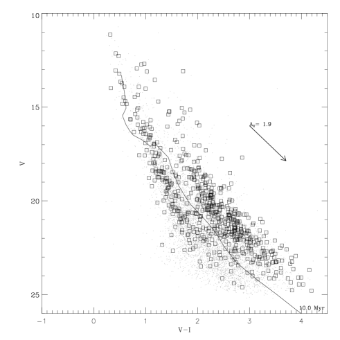
Figure 4: V vs. V-I diagram of all objects with optical magnitudes in our catalog. Class II YSOs are indicated with squares. Solid line is the 10 Myr solar metallicity isochrone of Siess et al. (2000) drawn assuming a distance of 3.6 kpc and E(B-V)=0.6.

5.2 Candidate diskless members

We define as diskless candidate members all the objects having an X-ray counterpart in the Chandra-ACIS catalog, showing any IR excess, i.e. not belonging to the sample of class II YSOs, defined in the previous section, and falling in the PMS region of the V vs. V-I diagram, i.e. that with colors redder than the 10 Myr solar metallicity isochrone of Siess et al. (2000) drawn assuming a distance of 3.6 kpc and E(B-V)=0.6 (see Sect. 6).

To define the PMS region, we have been guided by the bulk of objects with X-ray counterpart, as shown in Fig. 5 which depicts the V vs. V-I diagram of all objects with optical magnitudes in our catalog. Stars with X-ray counterpart are indicated with $\times$ symbols.

In the sample of diskless candidate members we also include the objects with X-ray emission that do not show any IR excess and have already reached the MS phase at the cluster age, i.e. those with V$<$15.

With the above conditions, we found 434 diskless YSOs, 85 of which are in the sample of 110 diskless YSOs found in Paper I. If we discard from the 110 diskless YSOs defined in Paper I the 17 objects considered here as class II YSOs, the remaining 8 diskless YSOs classified in Paper I do not have either V or I magnitudes. By using the literature B and V magnitudes by Massey et al. (1995) of these 8 objects, we found that 5 fall in the cluster MS region while the other 3 lie in the PMS region: we therefore included them in our sample of diskless cluster candidate members.

In summary, we have a total of 442 diskless YSOs. These objects are indicated with filled circles in the V vs. V-I diagram presented in Fig. 5.

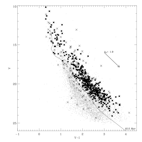
Figure 5: V vs. V-I diagram of all objects with optical magnitudes in our catalog. X-ray detections are indicated with $\times$ symbols while those selected as diskless YSOs are indicated with filled circles. Solid line is as in Fig. 4.

5.3 H_α emitters

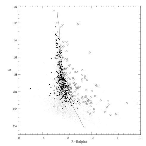
Figure 6: R vs. R-H_α diagram of all objects; diskless YSOs are indicated with filled circles while H_α emitters with at least an other membership indication are indicated as empty circles. Solid line is the limit we defined to distinguish diskless YSOs from high H_α emitters.

In the case of stars with accretion from circumstellar disk, the H_α line is much enlarged and therefore the (R-H_α) index is a measure of the H_α flux in excess. In order to identify stars with H_α emission, we used the R vs. R-H_α diagram shown in Fig. 6, where we defined the normal star limit by performing a linear fit of the R magnitudes of all diskless YSOs (indicated with filled circles) having R-H${}_{\alpha}<-3$. Then we estimated a typical error in the R-H_α index per bin of 0.5 magnitudes, as the average of the R-H_α errors in each bin. We added such errors to the R-H_α derived from the linear fit to obtain the limit indicated in the figure by the solid line. We defined as H_α emitters, those with R-H_α larger within 3 $\sigma$ than this limit. Among the 269 objects that satisfy this condition we consider as cluster H_α emitters only the 125 stars (indicated in the figure as empty circles) for which we have an additional membership indication, viz. 98 class II and 27 objects previously classified as diskless candidate members.

We included in the class II sample these 27 H_α emitters, that we had classified as diskless in the previous section. We note that this is not a contradiction in the classification but only a limit in the selection of candidate members with disk since there is a region in which the excesses by disks cannot be distinguished from reddened objects.

In summary, we have a sample of 1061 class II candidate members, 125 of which are H_α emitters, plus 415 diskless stars. Optical photometry and classification of class II and diskless candidates members are given in Tables 5 and 6 while new JHK photometry and Spitzer-IRAC magnitudes from Paper I of class II and diskless candidates members are given in Tables 7 and 8. 6

Table 5: Optical photometry of Class 0/I and Class II candidate members

Seq.	X ID	RA(2000)	Dec(2000)	V	R	I	Hα
Num.		[deg]	[deg]
1	55	80.6220775	33.5139642	9.045$\pm$ 0.016	9.241$\pm$ 0.047		0.036
2	779	80.7594680	33.5270160	11.132$\pm$ 0.014	10.978$\pm$ 0.017	10.817$\pm$ 0.011	0.009
3	664	80.7418460	33.4434210	12.147$\pm$ 0.014	11.923$\pm$ 0.050	11.725$\pm$ 0.016	0.009
4	276	80.6880800	33.4065610	12.269$\pm$ 0.010	12.034$\pm$ 0.035	11.793$\pm$ 0.011	0.014
5	…	80.7888715	33.5006385	12.692$\pm$ 0.022	12.103$\pm$ 0.007	11.721$\pm$ 0.013	0.037
6	…	80.6358343	33.5480553	12.733$\pm$ 0.025		11.819$\pm$ 0.006
7	887	80.7798330	33.5475840	12.938$\pm$ 0.011	12.491$\pm$ 0.008	12.110$\pm$ 0.014	0.009
8	345	80.6968720	33.4187280	13.047$\pm$ 0.011		12.628$\pm$ 0.039
9	773	80.7583743	33.5198142	13.084$\pm$ 0.015	12.211$\pm$ 0.016	11.365$\pm$ 0.021	0.007
10	…	80.7442230	33.5280269	13.105$\pm$ 0.007	12.588$\pm$ 0.025	12.083$\pm$ 0.022	0.006
…

• Notes - This table is published in its entirety in the electronic edition of Astronony & Astrophysics. A portion is shown here for guidance regarding its form and content.

7

Table 6: Optical photometry of diskless candidate members

Seq.	X ID	RA(2000)	Dec(2000)	V	R	I	Hα
Num.		[deg]	[deg]
1069	246	80.6833230	33.4407100	10.207$\pm$ 0.042		9.904$\pm$ 0.011
1070	281	80.6885760	33.3713500	10.724$\pm$ 0.009	10.605$\pm$ 0.008	10.254$\pm$ 0.020	0.035
1071	266	80.6865470	33.4434930	11.324$\pm$ 0.034		10.978$\pm$ 0.013
1072	11	80.5768170	33.4725590	11.716$\pm$ 0.019		11.412$\pm$ 0.038
1073	5	80.5541260	33.5671010	12.154$\pm$ 0.012		11.487$\pm$ 0.025
1074	362	80.6991250	33.3685801	12.451$\pm$ 0.006	12.004$\pm$ 0.012	11.398$\pm$ 0.014	0.041
1075	305	80.6923210	33.4224650	12.476$\pm$ 0.020		11.913$\pm$ 0.022
1076	651	80.7396750	33.4333360	12.710$\pm$ 0.016	12.465$\pm$ 0.030	12.180$\pm$ 0.019	0.006
1077	420	80.7068503	33.4259343	12.741$\pm$ 0.018		12.196$\pm$ 0.011
1078	155	80.6625410	33.4408110	13.123$\pm$ 0.022		12.422$\pm$ 0.006
…

• Notes - This table is published in its entirety in the electronic edition of Astronony & Astrophysics. A portion is shown here for guidance regarding its form and content.

8

Table 7: NIR photometry of Class 0/I and Class II candidate members

Seq.	RA(2000)	Dec(2000)	J	H	K	[3.6]	[4.5]	[5.8]	[8.0]
Num.	[deg]	[deg]
1	80.6220775	33.5139642				8.290$\pm$ 0.053	8.196$\pm$ 0.036	8.179$\pm$ 0.001	8.206$\pm$ 0.036
2	80.7594680	33.5270160	10.468$\pm$ 0.016		10.583$\pm$ 0.027	10.326$\pm$ 0.041	10.219$\pm$ 0.001	10.099$\pm$ 0.004	9.718$\pm$ 0.015
3	80.7418460	33.4434210	11.781$\pm$ 0.043	12.814$\pm$ 0.089	11.746$\pm$ 0.019	11.045$\pm$ 0.002	10.905$\pm$ 0.002	10.802$\pm$ 0.005	10.662$\pm$ 0.016
4	80.6880800	33.4065610	11.574$\pm$ 0.016	11.519$\pm$ 0.019	11.306$\pm$ 0.008	11.331$\pm$ 0.002	11.255$\pm$ 0.002	11.373$\pm$ 0.017	11.399$\pm$ 0.051
5	80.7888715	33.5006385	10.905$\pm$ 0.039	10.434$\pm$ 0.029	10.116$\pm$ 0.018	9.262$\pm$ 0.041	8.894$\pm$ 0.042	8.568$\pm$ 0.002	8.380$\pm$ 0.003
6	80.6358343	33.5480553	11.859$\pm$ 0.070	11.430$\pm$ 0.059	11.477$\pm$ 0.061	10.686$\pm$ 0.001	10.747$\pm$ 0.001	10.726$\pm$ 0.005	10.811$\pm$ 0.025
7	80.7798330	33.5475840	11.403$\pm$ 0.036	11.630$\pm$ 0.048	11.099$\pm$ 0.036	10.927$\pm$ 0.001	10.959$\pm$ 0.001	10.963$\pm$ 0.009	10.992$\pm$ 0.026
8	80.6968720	33.4187280	12.439$\pm$ 0.016	12.501$\pm$ 0.034	12.326$\pm$ 0.013	11.992$\pm$ 0.016		11.971$\pm$ 0.036	11.845$\pm$ 0.079
9	80.7583743	33.5198142				9.367$\pm$ 0.041	9.376$\pm$ 0.048	9.295$\pm$ 0.002	9.348$\pm$ 0.010
10	80.7442230	33.5280269				10.697$\pm$ 0.002	10.654$\pm$ 0.002	10.517$\pm$ 0.017	10.015$\pm$ 0.054
…

• Notes - This table is published in its entirety in the electronic edition of Astronony & Astrophysics. A portion is shown here for guidance regarding its form and content.

9

Table 8: NIR photometry of diskless candidate members

Seq.	RA(2000)	Dec(2000)	J	H	K	[3.6]	[4.5]	[5.8]	[8.0]
Num.	[deg]	[deg]
1069	80.6833230	33.4407100		9.394$\pm$ 0.053	9.532$\pm$ 0.043	9.559$\pm$ 0.027	9.605$\pm$ 0.040	9.580$\pm$ 0.003	9.658$\pm$ 0.010
1070	80.6885760	33.3713500	10.041$\pm$ 0.021	9.906$\pm$ 0.019		9.840$\pm$ 0.039	9.914$\pm$ 0.001	9.903$\pm$ 0.002	9.924$\pm$ 0.009
1071	80.6865470	33.4434930	10.545$\pm$ 0.025	10.508$\pm$ 0.018	10.628$\pm$ 0.012	10.582$\pm$ 0.002	10.574$\pm$ 0.002	10.637$\pm$ 0.009	10.697$\pm$ 0.029
1072	80.5768170	33.4725590	11.348$\pm$ 0.035	11.103$\pm$ 0.035	10.982$\pm$ 0.014	10.957$\pm$ 0.001	10.946$\pm$ 0.001	10.954$\pm$ 0.006	11.029$\pm$ 0.023
1073	80.5541260	33.5671010	10.811$\pm$ 0.020	10.577$\pm$ 0.027	10.545$\pm$ 0.010	10.506$\pm$ 0.035	10.449$\pm$ 0.001	10.503$\pm$ 0.005	10.539$\pm$ 0.017
1074	80.6991250	33.3685801				10.259$\pm$ 0.070	10.395$\pm$ 0.001	10.375$\pm$ 0.004	10.370$\pm$ 0.014
1075	80.6923210	33.4224650	11.485$\pm$ 0.017	11.361$\pm$ 0.019	11.266$\pm$ 0.009	11.316$\pm$ 0.014	11.289$\pm$ 0.071	11.259$\pm$ 0.030	11.136$\pm$ 0.062
1076	80.7396750	33.4333360	11.667$\pm$ 0.022	11.442$\pm$ 0.023	11.349$\pm$ 0.012	11.177$\pm$ 0.002	11.143$\pm$ 0.002	11.160$\pm$ 0.007	11.102$\pm$ 0.022
1077	80.7068503	33.4259343	12.128$\pm$ 0.094	12.254$\pm$ 0.150	11.851$\pm$ 0.105	11.481$\pm$ 0.004	11.512$\pm$ 0.005	11.302$\pm$ 0.049	11.431$\pm$ 0.040
1078	80.6625410	33.4408110	11.902$\pm$ 0.017	11.711$\pm$ 0.018	11.628$\pm$ 0.010	11.494$\pm$ 0.001	11.490$\pm$ 0.002	11.474$\pm$ 0.009	11.497$\pm$ 0.023
…

• Notes - This table is published in its entirety in the electronic edition of Astronony & Astrophysics. A portion is shown here for guidance regarding its form and content.

6 Cluster parameters

Metallicity, interstellar reddening and cluster distance are fundamental to compare the observed CMD with theoretical tracks and isochrones from which we estimate masses and ages of cluster candidate members. However, as already discussed in several papers (e.g. Hillenbrand, 1997; Gullbring et al., 1998), class II YSOs typically experience accretion phenomena, scattering and/or reflection processes due to the dust grains in their circumstellar disks that may alter their photospheric colors, also in the optical bands. In such cases comparison of observed magnitudes and colors with models can be unreliable and the results should be interpreted with caution. In order to get around this problem, we derive cluster parameters by considering only cluster candidate members without circumstellar disk (class III YSOs) for which the observed colors can be directly compared with evolutionary tracks and isochrones once the interstellar reddening is taken into account.

6.1 Metallicity

In this work we adopt models computed for solar metallicity, since there are ambiguous indications in the literature about the metallicity in NGC 1893. In a paper focused on the Galactic metallicity, Rolleston et al. (1993) and Rolleston et al. (2000) derived C, N, O, Mg, Al and Si abundances of 80 B-type main sequence stars, 8 of which are NGC 1893 members. After discarding two high rotator objects, they performed an LTE analysis from which they derive for NGC 1893 only a slight indication of under solar abundance. More recently, Daflon & Cunha (2004) derived non-LTE chemical abundances in young OB stars from high-resolution echelle spectra. The two NGC 1893 cluster members show again a marginal indication of subsolar metallicity, but from the chemical analysis of 69 young stars with Galactocentric distances between 4.7 and 13.2 kpc, Daflon & Cunha (2004) find metallicity slopes consistent with a flattening of the radial gradient. Even if Rolleston et al. (2000) found indication of steeper slopes, the available studies do not show strong evidence of sub-solar metallicity and therefore, as assumed in previous studies, we adopt a solar metallicity for NGC 1893.

6.2 Interstellar reddening

Color-color diagram using UBV photometry is the classical tool to derive the mean interstellar reddening of a given cluster by comparing expected photospheric colors with those observed for diskless cluster members. Fig. 7 shows the U-B vs. B-V diagram obtained by using literature UBV photometry by Massey et al. (1995) and Sharma et al. (2007); diskless stars are indicated with filled circles. We find that most of the bluest diskless YSOs, indicated by empty squares, are compatible with a reddening E(B-V)=0.6$\pm$0.1 from the comparison with the solar metallicity ZAMS of Siess et al. (2000), transformed into the observed colors by using the Kenyon & Hartmann (1995) relations. Diskless candidate members with B-V$\gtrsim$0.6 can be compatible with lower reddenings, down to E(B-V)=0.2, or with higher reddenings, at least up to E(B-V)=1.3, as shown by the ZAMS reddened with E(B-V)=0.2 and E(B-V)=1.3 (dashed lines in Fig. 7).

Figure 7: U-B vs. B-V diagram obtained by using Massey et al. (1995) and Sharma et al. (2007) photometry (dots); filled circles are diskless candidate members, squares are those compatible with reddening $0.5<E(B-V)<0.7$ based on the expected photospheric colors by Kenyon & Hartmann (1995) drawn at the E(B-V) values indicated on each line. The reddening vector obtained using the Munari & Carraro (1996) reddening law is also shown.

This allows us to deduce that the cluster region is affected by a significant differential reddening and that for the reddest objects the interstellar reddening cannot be photometrically derived. On the contrary, it can be unequivocally derived for the bluest objects, i.e. those indicated with squares for which the $0.5<$E(B-V)$<0.7$. This result has been checked by computing individual reddenings for the 12 diskless YSOs with U-B$\lesssim 0.5$ for which spectral types are available (Hiltner, 1966; Massey et al., 1995; Marco & Negueruela, 2002); we found that among the bluest objects (B-V$\lesssim$0.5), all the reddening values are compatible with E(B-V)=0.6$\pm$0.1, while among the reddest ones (B-V$\gtrsim$0.5), four have E(B-V)$\sim$0.2 and one has E(B-V)=0.68.

The mean reddening E(B-V)=0.6$\pm$0.1 we derive for NGC 1893 is consistent also in the V vs. V-I CMD shown in Fig. 8. In this figure, dots indicate all objects in the FoV with error in V-I smaller than 0.1 and filled circles indicate diskless candidate cluster members. Objects indicated also with squares are those with E(B-V) between 0.5 and 0.7, as in Fig. 7. The thick line is the solar metallicity ZAMS of Siess et al. (2000) at a distance of 3.6 kpc (see Sect. 6.3) and reddened using E(B-V)=0.4. The value E(B-V)=0.4 is that assumed for foreground objects that we expect to be less reddened than cluster members. To fit the highest mass range not covered by the Siess et al. (2000) ZAMS, we use the theoretical isochrone at solar metallicity of 1.5 Myr of Marigo et al. (2008) reddened with E(B-V)=0.5, 0.6 and 0.7 at a distance of 3.6 kpc (dashed lines). In this diagram, diskless candidate cluster members show a large spread that can be due to several reasons, such as differential reddening, binarity and/or age spread. This is true also in the V$\lesssim 16$ range where we can have objects in PMS or MS phase. However, those with 0.5$<$E(B-V)$<$0.7, as derived from Fig. 7 (indicated with squares) are well fitted by the 1.5 Myr isochrone if a reddening E(B-V)=0.6$\pm$0.1 is adopted, in agreement with the value we derived by using the U-B vs. B-V diagram. On the contrary, the other bright objects show a significant spread and can be both PMS objects or very reddened MS members. We note also that the choice of the 1.5 Myr isochrone is not critical for this result since in this mass range, isochrones degenerate in a vertical shape branch. For this reason in the V vs. V-I diagram, MS members cannot be used to constrain neither ages, nor the cluster distance, while they can constrain the cluster reddening.

Our result is also consistent in the low mass range, as can be seen by using the V-I vs J-K diagram shown in Fig. 9, where we present the color-color diagram of all objects; diskless candidate members are used to estimate the cluster reddening by considering the locus of expected photospheric colors by Kenyon & Hartmann (1995); we take advantage of the fact that in this diagram the expected photometric colors for low mass stars are almost vertical.

In order to estimate the cluster reddening, we considered also the distribution of the J-K colors of diskless candidate members within fixed ranges of 0.2 magnitudes in the interval $1.3<$V-I$<3.0$, and we considered, for each V-I bin, the peaks of the J-K distribution to derive the fiducial cluster sequence, indicated by the error bars in the bottom panel of Fig. 9. Comparison of this fiducial sequence with the lines allows us to confirm that the NGC 1893 mean reddening is E(B-V)=0.6$\pm$0.1. However, since the population of low mass stars is larger and spatially spread over the whole region affected by a larger differential reddening, we note that low mass candidate cluster members can individually have E(B-V) larger or smaller values. As it will be shown later, by using IR colors we estimate that the reddening in this region is not larger than about E(B-V)=1.3 (A_V=4 mag).

The spread of low mass candidate cluster members in the V vs. V-I diagram is not due only to differential reddening. In fact, if we select the sample of low mass diskless candidate members from the V-I vs J-K diagram with 0.5$<$E(B-V)$<0.7$, we find that in the V vs. V-I diagram they show the same spread as all diskless and therefore we conclude that the low mass star spread in the V vs. V-I diagram could be also due to an intrinsic age spread and/or binarity.

We note that the E(B-V) value we derived both for low and high mass candidate cluster members, is independent of other adopted parameters such as distance, ages and metallicity. However further spectroscopic observations should be obtained to derive spectral types and therefore individual reddening values.

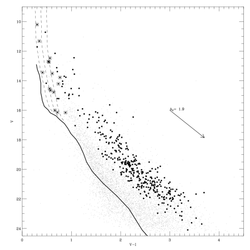
Figure 8: V vs. V-I diagram of all the objects (dots) with errors in V-I smaller than 0.1. Filled circles are the diskless candidate cluster members while squares indicate those with E(B-V) between 0.5 and 0.7, according to Fig. 7. Solid line is the solar metallicity ZAMS of Siess et al. (2000) at a distance of 3.6 kpc and reddening E(B-V)=0.4. Dashed lines indicate the 1.5 Myr Marigo et al. (2008) isochrone of solar metallicity for masses larger than 2 M_⊙ at 3.6 kpc and for E(B-V)=0.5, 0.6 and 0.7. The reddening vector obtained using the Munari & Carraro (1996) reddening laws is also shown.

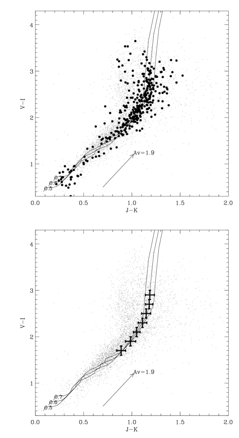
Figure 9: Color-color diagram of objects with error in color smaller than 0.1 (dots); solid lines are the photospheric colors by Kenyon & Hartmann (1995) at the three E(B-V) values indicated on each line. Filled circles in the upper panel are the NGC 1893 candidate cluster members without circumstellar disk while error bars in the bottom panel indicate the cluster sequence fiducial line derive as described on the text. The reddening vector obtained using the Munari & Carraro (1996) and Rieke & Lebofsky (1985) reddening laws is also shown.

6.3 Distance

The distance of NGC 1893 is a very uncertain parameter ranging in the literature from 3.2 to 6.0 kpc (see Sect. 7). Using broad band optical or NIR photometry of candidate cluster members and the isochrone fitting method, it is very difficult to derive the cluster distance. In fact, very young clusters such as NGC 1893 include a population of PMS stars, that lies in a ample region of the CMD diagram, and a small population, more or less rich, depending on the cluster age, of higher mass objects already on the MS phase and therefore on a well defined locus of the CMD. Nevertheless, the MS star distribution on the CMD is usually almost vertical and therefore quite ineffective for an accurate distance derivation. In addition, for clusters younger than about 15 Myr, the flattening of the isochrones between the two phases (PMS and MS) ends on the MS at a given magnitude that is strongly dependent on the isochrone age. Unfortunately, unless individual ages of PMS cluster members are well known, it is very hard to constrain the cluster distance by looking for this magnitude, even if the cluster mean reddening is fixed and a large population of high and low mass cluster members is known.

However, in the V vs. U-B diagram, the MS population is quite well separated from the bulk of the remaining objects that are field stars and candidate PMS cluster members. This is evident in the upper panels of Fig. 10, obtained by using the UBV photometry by Massey et al. (1995) and Sharma et al. (2007), and where diskless candidate cluster members selected by us are indicated with filled circles. Among these objects, we indicate with squares those that according to the U-B vs. B-V diagram have 0.5$<$E(B-V)$<$0.7. We use these objects here to constrain the cluster distance by comparing again the solar metallicity isochrone of 1.5 Myr of Marigo et al. (2008) reddened with E(B-V)=0.6. By taking advantage of the slightly curved shape of the isochrone in this CMD, we find that a good fitting is achieved if a distance of 3.6 kpc is adopted with an error of about 200 pc. With our data, we can rule out for NGC 1893 a distance of 3200 pc or 4300 pc that are values previously given in the literature (Sharma et al., 2007; Tapia et al., 1991; Massey et al., 1995).

A distance of 3.6 kpc for NGC 1893 is also consistent with that derived by using an independent method based on the nebula properties. In fact, as already done in previous works (Prisinzano et al., 2005; Guarcello et al., 2007), we assume that the nebula surrounding the cluster obscures many background objects and allows us to see mainly foreground stars, that are mostly in MS, with distance smaller or equal to the nebula distance. Among these latter, those located at the nebula distance define the blue envelope of the CMD diagram that can be fitted by the ZAMS locus. In the plausible assumption that the nebula is located at the same distance of NGC 1893 and by considering only very high reddened regions around the cluster (to minimize the spread due to background objects), it is possible to derive the cluster distance by fitting the ZAMS to the blue envelope of the CMD.

By a visual inspection of our observations in the optical, JHK and Spitzer/IRAC bands, we note that the nebula is not evenly spatially distributed, lying mostly in the western region of our FoV. For this reason, we selected the MS stars to be used for the ZAMS isochrone fitting by using the most obscured regions. The latter have been selected by means of a reddening map based on the distribution of the H-K colors, as done in Damiani et al. (2006, see this paper for details) by using H-K=0.1 as limit for the intrinsic color expected for background giants. As in Damiani et al. (2006), for the map computation we excluded all objects classified as candidate cluster members. The A_V map has been derived by using a cell size of 3.1^′$\times$ 2.6^′  within the FoV defined by our NICS/JHK observations and by the E(K-H) map, obtained as the median of H-K colors in each cell minus the expected 0.1 value. We find that the whole region is affected by $2.2\lesssim{\rm A}_{\rm V}\lesssim 4$, with the reddest regions being the western ones. As already mentioned, the whole region is not affected by very high A_V values and this can be also confirmed by the distribution of field stars in the J-H vs. H-K diagrams. This is likely due to a low absolute reddening affecting the galactic anti-center direction.

By using the resulting A_V map, we selected all the objects within the regions with A${}_{\rm V}>3.8$ and error in the V-I colors smaller than 0.1; the CMD diagram of these objects (indicated with dots) is shown in the bottom panels of Fig. 10, where filled circles are diskless candidate members. The dashed curve in the figure represents the solar metallicity ZAMS of Siess et al. (2000) shifted at the distance d=3.6 kpc and using E(B-V)=0.4, that is the minimum reddening we associate to field stars according to the bright stars in this diagram, while the solid line is the solar metallicity 1.5 Myr isochrone of Marigo et al. (2008) for stars with mass M$>$1.5M_⊙, adopting the same distance and E(B-V)=0.6, that is the mean cluster reddening we derived in the previous section.

As already mentioned, we derive the cluster distance as that value for which a good ZAMS fitting to MS stars of the blue envelope of this diagram is achieved. We note that, since the maximum A_V is about 4, even in the most obscured regions, a little fraction of faint background objects could be visible. In fact, as shown in Fig.10 (bottom panel), objects with V$>21$ do not follow the ZAMS shape, likely because this region is populated by field stars or extragalactic objects, that are expected to be visible in the galactic anti-center direction where the cluster NGC 1893 is located. Therefore, for the ZAMS fitting we consider only field stars with V$<21$; nevertheless, since the bright population of field stars (V$\lesssim 17$) is poorly populated, we considered, in this range, the candidate cluster members with $V\lesssim 16$ that are on the MS phase and with 0.5$<$E(B-V)$<$0.7, indicated with squares. We note that V$\simeq 16$ is the magnitude of the Turn On, i.e. the magnitude where the PMS joins the cluster MS. We fitted the candidate MS cluster members assuming the mean cluster reddening E(B-V)=0.6 and we found that a good fit is obtained both for the MS stars in the blue envelope and for the bright candidate cluster members on MS if a distance of $\sim$3.6 kpc (see bottom panel of Fig.10) is used. By taking the solar galactocentric distance of 8.5 Kpc, we deduce that NGC 1893 is located at a distance of about 12.1 Kpc from the Galactic Center.

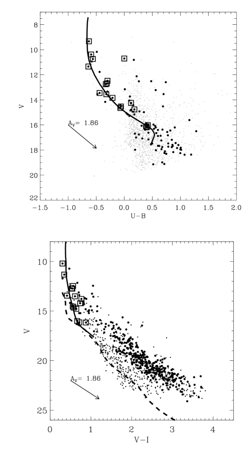
Figure 10: V vs. U-B diagram from the Massey et al. (1995) and Sharma et al. (2007) photometry (upper panels) and V vs. V-I diagram of all the objects with errors in V-I smaller than 0.1 and located in the regions with A${}_{\rm V}>3.8$ (bottom panels). Filled circles are the diskless candidate cluster members; squares are those with 0.5$<$E(B-V)$<$0.7; solid line is the 3.0 Myr isochrone of solar metallicity using E(B-V)=0.6 while dashed line is the solar metallicity ZAMS of Siess et al. (2000) using E(B-V)=0.4; both are drawn assuming a distance of 3.6 kpc. The reddening vector obtained using the Munari & Carraro (1996) reddening laws is also shown.

7 Comparison with literature cluster parameters

The cluster distance we derived (3.6$\pm$0.2 kpc) is marginally consistent with that recently derived by Sharma et al. (2007) (d=3250 pc) by fitting the 4 Myr isochrone of Bertelli et al. (1994) to the MS field stars and assuming E(B-V)=0.4, that is the value taken for the MS field stars. This method is similar to that used by us, since we note that the 4 Myr isochrone of Bertelli et al. (1994) corresponds rather to the ZAMS locus, if we consider that stars 4 Myr old with masses smaller than about 2 M_⊙ are yet in PMS.

We find a good agreement with the value derived by Cuffey (1973) who, using UBV magnitudes, derived that the reddening in front of the cluster amount to E(B-V)=0.4, while the distance is 3.6 kpc. Among the first distance values published for NGC 1893, Becker & Fenkart (1971) found d=3700 pc and A${}_{\rm V}=1.68$, corresponding to E(B-V)=0.54, by using simultaneously two color-magnitude diagrams. Moffat (1972) derived a distance of 3980 pc and a reddening E(B-V)=0.55 using photographic UBV photometry and the ZAMS fitting to the unreddened CMD. Humphreys (1978) found a distance modulus of 12.52 corresponding to a distance of about 3200 pc, by using V, B-V photometry of three O type main sequence stars of NGC 1893 in a paper devoted to study fundamental properties of the most luminous stars in our Galaxy.

A larger distance of 4300 pc has been derived by Tapia et al. (1991) by using Str$\ddot{\rm{o}}$mgren $ubvy$, H$\beta$ and JHK photometry. They derived spectral types and approximate luminosity classes from the $m_{1}$ and $c_{1}$ indices that together with literature slit spectral types are used to estimate reddening and absorption and therefore intrinsic colors and magnitudes for candidate cluster members. The corrected distance modulus is derived as the difference between the unabsorbed V magnitude and the absolute magnitude predicted for the given spectral type. A similar value, equal to 4800 pc, has been found by Fitzsimmons (1993), by using again Str$\ddot{\rm{o}}$mgren $ubvy$ photometry and the theoretical ZAMS fitting.

CCD UBV photometry and multiobject fiber spectroscopy are used by Massey et al. (1995) to determine distance and reddening equal to 4400 pc and E(B-V)=0.53$\pm$0.2, respectively. These values are derived by using individual reddening from spectroscopy and appropriate spectral type-M_V calibration for O and B-type stars. The derived distance has been obtained by including only stars with inferred color excess E(B-V) between 0.41 and 0.70

Vallenari et al. (1999) use J and K photometry and UBV literature photometry to derive E(J-K) from 0.15 to 0.5, corresponding to 0.25$<$E(B-V)$<$0.8 in the whole region they study; in addition they find two main dark regions where E(J-K) is 0.45-0.55 (or E(B-V)=0.7-0.9) that is higher than the value derived in the regions outside the dark clumps.

The most discordant distance value for NGC 1893 with respect to that found in this paper is that derived by Marco et al. (2001) equal to 6000 pc; they use photometric Str$\ddot{\rm{o}}$mgren indices (magnitude limit V$\simeq$15.9) to compute the interstellar reddening $E(b-y)$ of cluster members. They find values up to $E(b-y)=$0.607 but they estimate the average interstellar reddening $E(b-y)=0.33\pm 0.03$ by considering only stars with $E(b-y)<0.4$. They use this average reddening to derive individual magnitudes and colors ($V_{0}$, $(b-y)_{0}$ and $c_{0}$). By fitting an empirical ZAMS in the M_V vs. $c_{0}$ diagram they derive a dereddened distance modulus of 13.9. Considering that the cluster is affected by a significant differential reddening, we suppose that the photometric intrinsic parameters derived by Marco et al. (2001), based on the average reddening could be the origin of their overestimate of the cluster distance.

8 Masses and Ages

Assuming the cluster parameters derived by us in the previous sections, we was able to compute masses and ages of all objects we selected as candidate cluster members. However, as we mentioned before, the position in the color-magnitude diagram of class II candidate members can be influenced by effects due to the presence of circumstellar disk. Since our data do not allow to disentangle the purely photospheric spectrum of the stars, to which theoretical models are referred, from that in excess due to such effects, we assume that masses and ages of diskless stars can be accurately derived within the uncertainties due to photometric errors, reddening and to the theoretical models, while masses and ages of class II stars should be taken with caution, especially those of the 170 candidate members falling outside the PMS region with ages apparently older than 10 Myr.

Masses and ages are computed by interpolating the solar metallicity Siess et al. (2000) tracks on the V vs. V-I plane, using the TRIGRID idl function. Figure 11 shows the V vs. V-I diagram with the Siess et al. (2000) tracks and isochrones superposed.

For the diskless sample we find stars with masses between 0.3 and 6.7 M_⊙; we have further 11 objects classified as diskless candidate members with mass larger than 7 M_⊙; the median value and the standard deviation of diskless member ages are 1.4 Myr and 1.8 Myr, respectively. For the class II sample, if we discard the 170 stars with optical anomalous photometry, we find stars with masses between 0.2 and 6.9 M_⊙; we have further 10 objects classified as class II candidate members with mass larger than 7 M_⊙; the median value and the standard deviation of ages of candidate members with disk are 1.6 Myr and 2.2 Myr, respectively, with again few stars being 9-10 Myr old. We conclude that, apart from the 170 objects with anomalous optical indices, the remaining class II stars show mass and age distributions very similar to those of diskless YSOs as it is shown in Fig. 12 where the age distribution of diskless and class II candidate members are shown. This reflects the similar spread observed in the V vs. V-I diagram by the two populations of candidate members. Apparently the colors of class II candidate members are not substantially modified by phenomena related to accretion. The peak in the observed mass function is among 0.4 and 0.5 $M_{\odot}$; however the IMF will be computed in an other work where we will discuss the biases due to the adopted methods and where we will compare the IMF with that of other clusters of similar age.

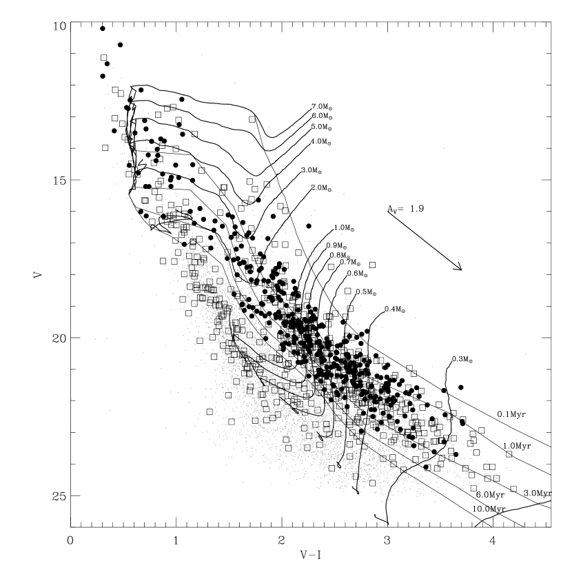
Figure 11: V vs. V-I diagram of all objects with optical magnitudes in our catalog (dots). diskless and class II candidate members are indicated with filled circles and empty squares, respectively. Lines are the Siess et al. (2000) tracks and isochrones of masses and ages indicated on each line.

Figure 12: Age distribution of diskless and class II candidate members in the PMS region. Class II YSOs with anomalous blue colors are not included in this sample.

9 Summary and conclusions

We used new deep optical NIR data in the VRIJHK and H_α bands together with literature X-ray and Spitzer-IRAC data to compile a multiband photometric catalog in the direction of the young distant open cluster NGC 1893, located towards the galactic anti-center. Using these data and different membership criteria, we made the most complete census of candidate members available in the literature for this cluster. Reddening-independent indices, involving optical and/or NIR colors, allowed us to derive a list of 1061 candidate members with a circumstellar disk, with 125 among them being also H_α emitters; among the disk bearing candidate members, 170 show anomalous optical magnitudes and colors that are likely due to effects of gas and/or dust in the disk. In addition, X-ray detections and optical magnitudes, allowed us to distinguish 415 candidate members without disk.

We used these last 415 YSOs and their photometric properties, to assess the cluster parameters, viz. interstellar reddening and distance. Disk-less candidate members are, in fact, the most reliable objects to be compared with theoretical tracks and isochrones, since their colors are purely photospheric and do not suffer from additional effects due to the presence of circumstellar disks.

Bright diskless members in the U-B vs. B-V diagram, obtained from literature data, are consistent with an interstellar reddening E(B-V)=0.6$\pm$0.1. This value is also consistent using the same bright candidate members in the independent V vs. V-I diagram and most of the low mass diskless candidate members in the V-I vs. J-K diagram. However, we find evidence of differential reddening in this region.

Using the V vs. B-V (from the literature) diagram, and assuming the mean cluster reddening E(B-V)=0.6, we find that the main sequence members selected in this work are well fitted by a 1.5 Myr isochrone, if a distance of 3.6$\pm$0.2 kpc is adopted. We note that in the MS cluster region, isochrones degenerate and therefore our distance estimate is independent of the age adopted for MS members. The value of 3.6 kpc is consistent with the cluster distance we derive by using the main sequence blue envelope traced in the V vs. V-I diagram by foreground field stars located at the cluster distance. Therefore, using independent methods and data, we are able to firmly evaluate the cluster distance for which values between 3250 and 6000 pc are given in the most recent literature.

Finally, we derived masses and ages of selected candidate members in the optical PMS region down to about 0.2 M_⊙; median ages for diskless and class II stars, are, respectively, 1.4 and 1.6 Myr, with a standard deviation of 1.8 and 2.2 Myr for the two samples. Few cluster candidate members are older with ages up to about 10 Myr.

If we consider that 1001 of the 1061 class II candidate members are within the Chandra FoV, where we have selected the diskless candidate members, we find a disk fraction of about 71% of stars. This value is an upper limit since the diskless member selection is based on the X-ray observations that reach a mass limit higher than that we can reach with NIR observations used to select class II stars. However, the disk fraction we find is similar to the 67% value we found in Paper I and in agreement with the disk fraction found in clusters of similar age (Haisch et al., 2001), if we assume for NGC 1893 a median age of 1.5 Myr. A detailed analysis of the disk fraction as a function of stellar masses and cluster location will be the subject of a forthcoming paper (Sanz-Forcada et al. 2010, in preparation).

We therefore conclude that, despite its peculiar location in the Galaxy, NGC 1893 includes a rich population of young stars, with general properties similar to those found in young clusters in the solar neighborhood.

Appendix A Photometric calibration

A.1 DOLORES

Photometric calibration of DOLORES observations was computed by using the images of the Landolt (1992) standard field SA 98. We used the v, r, i, h_α instrumental magnitudes, and considered the V, R and I magnitudes of the Johnson-Kron-Cousins photometric system of standard stars in these fields (Stetson 2000); H_α is the magnitude in the corresponding non-standard filter. We calculated the transformation coefficients between the instrumental and standard systems by using the CCDSTD code (Stetson 2005) and the following equations:

$$v = V+A_{0}+A_{1}\,Q+A_{2}\,(V-I)+A_{3}\,(V-I)^{2}+A_{4}\,X\,Y+$$

$$+A_{5}\,X+A_{6}\,Y+A_{7}\,X^{2}+A_{8}\,Y^{2}$$

$$r = R+B_{0}+B_{1}\,Q+B_{2}\,(R-I)+B_{3}\,(R-I)^{2}+B_{4}\,X\,Y+$$ (3)

$$+B_{5}\,X+B_{6}\,Y+B_{7}\,X^{2}+B_{8}\,Y^{2}$$

$$i = I+C_{0}+C_{1}\,Q+C_{2}\,(V-I)+C_{3}\,(V-I)^{2}+C_{4}\,X\,Y+$$

$$+C_{5}\,X+C_{6}\,Y+C_{7}\,X^{2}+C_{8}\,Y^{2}$$

$$h_{\alpha} = H_{\alpha}+D_{0}+D_{1}\,Q+D_{2}\,(R-I)+D_{3}\,(R-I)^{2}+D_{4}\,X\,Y+$$

$$+D_{5}\,X+D_{6}\,Y+D_{7}\,X^{2}+D_{8}\,Y^{2}$$

where $Q$ is the airmass, $A_{0}$, $B_{0}$ and $C_{0}$ are the magnitude zero points; $A_{1}$, $B_{1}$ and $C_{1}$ are the extinction coefficients; $A_{2}$, $B_{2}$ and $C_{2}$ and $A_{3}$, $B_{3}$ and $C_{3}$ are the color terms, and the rest of terms are related to the geometrical coordinates ($X,Y$) of the plate. Stars with magnitude residual values above the 3$\sigma$ level were not considered for the coefficient fitting. Coefficients calculated during calibration are listed in Table 10. DOLORES extinction terms are set to those provided by the telescope web site. We followed the same nomenclature for the H$\alpha$ filter, but since we have no standard measurements in this band, we applied the same calibration as for the R band (therefore $D_{i}=C_{i}$) in the case of DOLORES.

Table 10: Coefficients of the transformations to the standard system, given in the Eq.s A.1, for each filter and night for DOLORES (D)^a and CAFOS (C)

Instr.	Date	Filter	Coeff.	$A_{i}$, $B_{i}$, $C_{i}$, $D_{i}$ coefficient indices
				0	1	2	3	4	5	6	7	8
D	2007/09/21	V	$A_{i}$	-0.874	0.15	0.087	…	…	-0.068	0.138	…	-0.045
				$\pm$0.014		$\pm$0.007	…	…	$\pm$0.006	$\pm$0.021	…	$\pm$0.010
D	”	R	$B_{i}$	-0.823	0.11	-0.002	…	…	-0.072	-0.007	…	…
	”			$\pm$0.008		$\pm$0.009	…	…	$\pm$0.004	$\pm$0.003	…	…
D	”	I	$C_{i}$	-0.531	0.07	-0.035	…	…	0.420	0.393	-0.191	-0.181
	”			$\pm$0.020		$\pm$0.006	…	…	$\pm$0.026	$\pm$0.017	$\pm$0.010	$\pm$0.008
D	2007/10/18	V	$A_{i}$	-1.039	0.15	0.103	…	…	-0.007	0.015	…	-0.006
				$\pm$0.004		$\pm$0.002	…	…	$\pm$0.002	$\pm$0.007	…	$\pm$0.003
D	”	R	$B_{i}$	-1.100	0.11	0.015	…	…	0.013	0.011	…	…
	”			$\pm$0.003		$\pm$0.004	…	…	$\pm$0.002	$\pm$0.002	…	…
D	”	I	$C_{i}$	-0.572	0.07	0.018	…	…	0.237	0.224	-0.081	-0.117
	”			$\pm$0.009		$\pm$0.004	…	…	$\pm$0.019	$\pm$0.010	$\pm$0.011	$\pm$0.005
D	2007/11/14	V	$A_{i}$	-1.019	0.15	0.090	…	…	-0.014	0.072	…	-0.026
				$\pm$0.013		$\pm$0.004	…	…	$\pm$0.016	$\pm$0.011	…	$\pm$0.005
D	”	R	$B_{i}$	-1.050	0.11	-0.007	…	…	0.043	0.002	-0.026	…
	”			$\pm$0.005		$\pm$0.004	…	…	$\pm$0.008	$\pm$0.002	$\pm$0.003	…
D	”	I	$C_{i}$	-0.537	0.07	-0.019	…	…	0.307	0.239	-0.136	-0.128
	”			$\pm$0.010		$\pm$0.004	…	…	$\pm$0.014	$\pm$0.010	$\pm$0.006	$\pm$0.005
C	2007/10/11	V	$A_{i}$	2.482	0.118	-0.022	0.015	-0.026	-0.236	-0.127	0.139	0.086
				$\pm$0.019	$\pm$0.004	$\pm$0.015	$\pm$0.005	$\pm$0.011	$\pm$0.022	$\pm$0.023	$\pm$0.010	$\pm$0.012
C	”	R	$B_{i}$	1.820	0.045	0.030	-0.056	-0.147	0.261	0.151	…	…
	”			$\pm$0.042	$\pm$0.011	$\pm$0.049	$\pm$0.031	$\pm$0.061	$\pm$0.082	$\pm$0.091	…	…
C	”	I	$C_{i}$	2.467	0.051	-0.082	-0.015	-0.039	0.206	0.344	-0.132	-0.208
	”			$\pm$0.021	$\pm$0.005	$\pm$0.009	$\pm$0.004	$\pm$0.025	$\pm$0.030	$\pm$0.040	$\pm$0.021	$\pm$0.022
C	”	Hα	$D_{i}$	-1.344	1.088	0.340	…	0.063	-0.333	-0.384	0.205	0.238
	”			$\pm$0.027	$\pm$0.323	$\pm$0.036	…	$\pm$0.014	$\pm$0.028	$\pm$0.029	$\pm$0.012	$\pm$0.016
C	2008/01/05	V	$A_{i}$	2.642	…	0.063	-0.012	-0.018	0.190	0.118	-0.094	-0.098
				$\pm$0.012	…	$\pm$0.011	$\pm$0.004	$\pm$0.008	$\pm$0.014	$\pm$0.013	$\pm$0.007	$\pm$0.007
C	”	R	$B_{i}$	1.940	…	0.038	-0.037	-0.010	0.201	0.129	-0.099	-0.131
	”			$\pm$0.010	…	$\pm$0.014	$\pm$0.008	$\pm$0.007	$\pm$0.012	$\pm$0.011	$\pm$0.005	$\pm$0.006
C	”	I	$C_{i}$	4.497	…	-0.108	-0.006	-0.222	-0.200	0.233	0.174	-0.043
	”			$\pm$0.021	…	$\pm$0.011	$\pm$0.003	$\pm$0.015	$\pm$0.027	$\pm$0.024	$\pm$0.013	$\pm$0.013
C	”	Hα	$D_{i}$	2.948	…	-0.373	0.374	0.027	-0.266	-0.594	0.162	0.347
	”			$\pm$0.105	…	$\pm$0.154	$\pm$0.127	$\pm$0.060	$\pm$0.130	$\pm$0.100	$\pm$0.052	$\pm$0.059
C	2008/01/09	Hα	$D_{i}$	1.724	…	0.045	-0.013	0.118	0.322	-0.266	-0.176	0.028
				$\pm$0.045	…	$\pm$0.051	$\pm$0.035	$\pm$0.026	$\pm$0.049	$\pm$0.050	$\pm$0.019	$\pm$0.024
Notes: aDOLORES observations in H$\alpha$ have same coefficients as for the R filter

A.2 CAFOS

We tried to calibrate the CAFOS observations following the same procedure as for DOLORES, using the site extinction terms as provided by Sánchez et al. (2007). However we noticed substantial discrepancies in the final magnitudes calculated for CAFOS when compared to DOLORES results. The variable atmospheric conditions detected during the observations, also noted in the seeing, could be responsible of the inconsistencies. We decided to use the DOLORES photometry to calibrate the CAFOS fields: we selected the local standards used in DOLORES fields that are also common to the CAFOS FoV, and used a total of 417 CAFOS counterparts as standards for the calibration, so we calibrated the CAFOS observations in the same photometric system of DOLORES. The second and third nights of CAFOS observations also required to set the “cloud” variable in the CCDSTD setting. As explained by Stetson (2000) this variable allows to consider different atmospheric conditions (thin clouds) during the night, setting all the extinction terms to 0 in this case (Table 10), and fitting the zero points and the other terms. CAFOS observations used the DOLORES standard stars falling in the field to calibrate the H$\alpha$ observations, with $D_{i}$ coefficients as listed in Table 10.

A.3 NICS

We used the standalone DAOPHOT II/ALLSTAR code (Stetson 1987b) to obtain the instrumental photometry for the combined images obtained with SNAP for each filter (JHK) and for each of the 16 fields observed around the cluster NGC 1893. For most of the images we performed the PSF photometry using the Moffat function with $\beta=2.5$, typically used to model stellar profiles as an analytic first approximation to the PSF, while for 6 images we used the more complex Penny function in order to take into account the elongated shape of the PSF likely due to some aberration. In addition we treated the variable PSF by using the DAOPHOT option that considers a PSF which varies quadratically with position in the frame.

Since the PSF photometry is relative to the model stellar profile of a given frame, we needed to derive the aperture correction to the instrumental photometry; to this aim we performed aperture photometry at different radii on a sample of isolated and relatively bright stars from which we derived growth curves with the DAOGROW code (Stetson 1990). The aperture correction has been computed using the selected stars as the median of the difference between the PSF magnitudes and the aperture magnitudes obtained at the radius including all the stellar flux.

In order to discard false identifications due to the spots either of very bright objects or just falling at the edge of the images, we selected the list of objects detected by considering only those following the typical exponential profile of the magnitude errors. Then for each of the 16 observed fields, we merged with DAOMATCH/DAOMASTER (Stetson 1987b) the three lists with JHK magnitudes in order to have a single list with objects having at least two among the JHK magnitudes.

The NICS filters used for our observations (Js, H, K’) are those of the Mauna Kea Observatories (MKO) near-infrared filter set (Ghinassi et al. 2002) and therefore we calibrate our catalog in the MKO photometric system. To this aim we use as standard stars, the 2MASS counterparts falling in our fields with PH_QUAL flag equal to ’AAA’ and CC_FLG flag equal to ’000’. We first converted the 2MASS catalog in the MKO system by using the inverted transformations given in the 2MASS web page maintened by J. Carpenter (see also Leggett et al. 2006).

By using instrumental magnitudes for the standard stars, that we indicate as j, h, k and those of the 2MASS catalog in the MKO system, that we indicate as J_MKO, H_MKO, K_MKO we performed for each field a linear fit of the magnitude differences as a function of the colors as in the following equations:

$${\rm(j-J_{MKO})=A_{0}+A_{1}(j-h)}$$

$${\rm(j-J_{MKO})=B_{0}+B_{1}(j-k)}$$

$${\rm(h-H_{MKO})=C_{0}+C_{1}(j-h)}$$ (4)

$${\rm(h-H_{MKO})=D_{0}+D_{1}(h-k)}$$

$${\rm(k-K_{MKO})=E_{0}+E_{1}(j-k)}$$

$${\rm(k-K_{MKO})=F_{0}+F_{1}(h-k)}.$$

From the linear fit we derived the zero points, indicated by coefficients with subscript 0 and the color terms, indicated by coefficients with subscript 1 given in Table 11.

Table 11: Zero points (coefficients with subscript 0) and color terms (coefficients with subscript 1) derived from the linear fit of equations (A.3) to transform instrumental NICS magnitudes to the MKO system.

f	A0	A1	B0	B1	C0	C1	D0	D1	E0	E1	F0	F1
1	-22.505	0.039	-22.487	0.027	-22.522	-0.056	-22.598	-0.108	-21.957	-0.007	-21.964	-0.015
	$\pm$ 0.013	$\pm$ 0.018	$\pm$ 0.007	$\pm$ 0.013	$\pm$ 0.015	$\pm$ 0.019	$\pm$ 0.015	$\pm$ 0.043	$\pm$ 0.009	$\pm$ 0.014	$\pm$ 0.015	$\pm$ 0.044
2	-22.577	0.064	-22.548	0.049	-22.740	0.014	-22.673	0.142	-22.178	0.072	-22.077	0.205
	$\pm$ 0.026	$\pm$ 0.040	$\pm$ 0.010	$\pm$ 0.028	$\pm$ 0.029	$\pm$ 0.044	$\pm$ 0.042	$\pm$ 0.099	$\pm$ 0.013	$\pm$ 0.034	$\pm$ 0.047	$\pm$ 0.114
3	-22.388	-0.014	-22.397	-0.004	-22.581	-0.039	-22.617	-0.020	-21.928	-0.010	-21.942	-0.024
	$\pm$ 0.025	$\pm$ 0.036	$\pm$ 0.009	$\pm$ 0.026	$\pm$ 0.029	$\pm$ 0.041	$\pm$ 0.048	$\pm$ 0.098	$\pm$ 0.010	$\pm$ 0.029	$\pm$ 0.043	$\pm$ 0.089
4	-22.410	-0.107	-22.459	-0.076	-22.519	-0.231	-22.757	-0.255	-22.079	-0.030	-22.148	-0.157
	$\pm$ 0.016	$\pm$ 0.028	$\pm$ 0.006	$\pm$ 0.022	$\pm$ 0.020	$\pm$ 0.032	$\pm$ 0.034	$\pm$ 0.082	$\pm$ 0.008	$\pm$ 0.025	$\pm$ 0.035	$\pm$ 0.083
5	-22.504	0.044	-22.485	0.034	-22.609	-0.101	-22.708	-0.100	-22.116	0.014	-22.128	-0.041
	$\pm$ 0.012	$\pm$ 0.019	$\pm$ 0.005	$\pm$ 0.015	$\pm$ 0.013	$\pm$ 0.020	$\pm$ 0.023	$\pm$ 0.058	$\pm$ 0.007	$\pm$ 0.017	$\pm$ 0.025	$\pm$ 0.063
6	-22.471	0.053	-22.450	0.048	-22.581	-0.053	-22.583	0.078	-22.081	0.056	-21.998	0.189
	$\pm$ 0.014	$\pm$ 0.022	$\pm$ 0.006	$\pm$ 0.017	$\pm$ 0.015	$\pm$ 0.025	$\pm$ 0.023	$\pm$ 0.060	$\pm$ 0.007	$\pm$ 0.017	$\pm$ 0.021	$\pm$ 0.056
7	-22.063	-0.023	-22.073	0.011	-22.074	-0.069	-22.076	0.094	-21.682	-0.004	-21.683	-0.001
	$\pm$ 0.010	$\pm$ 0.024	$\pm$ 0.005	$\pm$ 0.018	$\pm$ 0.013	$\pm$ 0.029	$\pm$ 0.015	$\pm$ 0.052	$\pm$ 0.006	$\pm$ 0.019	$\pm$ 0.014	$\pm$ 0.049
8	-22.627	0.257	-22.493	0.198	-22.670	-0.067	-22.664	0.114	-22.145	0.246	-22.510	-0.891
	$\pm$ 0.025	$\pm$ 0.035	$\pm$ 0.011	$\pm$ 0.037	$\pm$ 0.029	$\pm$ 0.037	$\pm$ 0.051	$\pm$ 0.105	$\pm$ 0.016	$\pm$ 0.048	$\pm$ 0.064	$\pm$ 0.133
9	-22.336	-0.023	-22.346	0.010	-22.450	-0.026	-22.260	0.580	-22.005	0.074	-21.918	0.242
	$\pm$ 0.014	$\pm$ 0.032	$\pm$ 0.006	$\pm$ 0.026	$\pm$ 0.017	$\pm$ 0.037	$\pm$ 0.037	$\pm$ 0.106	$\pm$ 0.007	$\pm$ 0.031	$\pm$ 0.047	$\pm$ 0.132
10	-22.409	-0.032	-22.428	-0.004	-22.557	-0.070	-22.562	0.109	-22.019	0.032	-21.980	0.078
	$\pm$ 0.016	$\pm$ 0.024	$\pm$ 0.007	$\pm$ 0.017	$\pm$ 0.019	$\pm$ 0.027	$\pm$ 0.020	$\pm$ 0.050	$\pm$ 0.009	$\pm$ 0.020	$\pm$ 0.019	$\pm$ 0.049
11	-22.358	0.057	-22.332	0.042	-22.553	0.005	-22.507	0.120	-21.969	0.078	-21.882	0.162
	$\pm$ 0.015	$\pm$ 0.020	$\pm$ 0.006	$\pm$ 0.013	$\pm$ 0.018	$\pm$ 0.023	$\pm$ 0.012	$\pm$ 0.031	$\pm$ 0.008	$\pm$ 0.013	$\pm$ 0.010	$\pm$ 0.028
12	-22.348	-0.091	-22.389	-0.079	-22.536	-0.144	-22.646	-0.034	-22.049	-0.012	-22.098	-0.110
	$\pm$ 0.025	$\pm$ 0.038	$\pm$ 0.010	$\pm$ 0.029	$\pm$ 0.028	$\pm$ 0.041	$\pm$ 0.047	$\pm$ 0.108	$\pm$ 0.013	$\pm$ 0.033	$\pm$ 0.052	$\pm$ 0.121
13	-22.469	0.123	-22.419	0.110	-22.531	-0.072	-22.412	0.441	-22.031	0.044	-21.936	0.224
	$\pm$ 0.032	$\pm$ 0.050	$\pm$ 0.012	$\pm$ 0.041	$\pm$ 0.039	$\pm$ 0.059	$\pm$ 0.063	$\pm$ 0.167	$\pm$ 0.019	$\pm$ 0.057	$\pm$ 0.077	$\pm$ 0.207
14	-22.401	0.029	-22.386	0.011	-22.551	-0.044	-22.661	-0.169	-21.939	0.080	-21.883	0.093
	$\pm$ 0.019	$\pm$ 0.032	$\pm$ 0.006	$\pm$ 0.025	$\pm$ 0.022	$\pm$ 0.035	$\pm$ 0.054	$\pm$ 0.107	$\pm$ 0.010	$\pm$ 0.032	$\pm$ 0.064	$\pm$ 0.129
15	-22.538	0.215	-22.436	0.176	-22.671	0.077	-22.502	0.272	-22.038	0.077	-21.966	0.133
	$\pm$ 0.021	$\pm$ 0.032	$\pm$ 0.008	$\pm$ 0.024	$\pm$ 0.022	$\pm$ 0.033	$\pm$ 0.032	$\pm$ 0.070	$\pm$ 0.009	$\pm$ 0.022	$\pm$ 0.030	$\pm$ 0.062
16	-22.489	0.067	-22.459	0.058	-22.554	-0.113	-22.565	0.138	-22.098	0.070	-22.000	0.203
	$\pm$ 0.026	$\pm$ 0.041	$\pm$ 0.008	$\pm$ 0.029	$\pm$ 0.031	$\pm$ 0.050	$\pm$ 0.044	$\pm$ 0.106	$\pm$ 0.011	$\pm$ 0.032	$\pm$ 0.041	$\pm$ 0.101

The final photometric catalog in the MKO system has been obtained by imposing these coefficients and the analogous equations to the instrumental magnitudes of all detected objects.