Probing interstellar turbulence in spiral galaxies using HI power spectrum analysis

Abstract

We estimate the H i  intensity fluctuation power spectrum for a sample of 18 spiral galaxies chosen from THINGS. Our analysis spans a large range of length-scales from $\sim 300\,{\rm pc}$ to $\sim 16\,{\rm kpc}$ across the entire galaxy sample. We find that the power spectrum of each galaxy can be well fitted by a power law $P_{\rm HI}(U)=A\ U^{\alpha}$, with an index $\alpha$ that varies from galaxy to galaxy. For some of the galaxies the scale-invariant power-law power spectrum extends to length-scales that are comparable to the size of the galaxy’s disk. The distribution of $\alpha$ is strongly peaked with $50\%$ of the values in the range $\alpha=-1.9$ to $1.5$, and a mean and standard deviation of $-1.3$ and $0.5$ respectively. We find no significant correlation between $\alpha$ and the star formation rate, dynamical mass, H i  mass or velocity dispersion of the galaxies.

Several earlier studies that have measured the power spectrum within our Galaxy on length-scales that are considerably smaller than $500\,{\rm pc}$ have found a power-law power spectrum with $\alpha$ in the range $\approx-2.8$ to $-2.5$. We propose a picture where we interpret the values in the range $\approx-2.8$ to $-2.5$ as arising from three dimensional (3D) turbulence in the Interstellar Medium (ISM) on length-scales smaller than the galaxy’s scale-height, and we interpret the values in the range $\approx-1.9$ to $-1.5$ measured in this paper as arising from two-dimensional ISM turbulence in the plane of the galaxy’s disk. It however still remains a difficulty to explain the small galaxy to galaxy variations in the values of $\alpha$ measured here.

1 Introduction

Scale-invariant structures seen in galaxies are believed to be the result of compressible turbulence. The source of the turbulence could be protostellar winds, supernova, rotational shear, spiral arm shocks, etc. (see Elmegreen and Scalo 2004 for a review). A variety of statistical measures have been proposed to characterize the structures seen in the ISM (see Lazarian and Pogosyan 2000; Padoan et al. 2001; Brunt and Heyer 2002; Lazarian and Pogosyan 2004; Burkhart et al. 2010). Of these, power spectrum is most popular. In the case of compressible turbulence the power spectrum is expected to have a power law shape, and the slope $\alpha$ of the power law contains information as to the nature of the turbulence.

In the case of the galactic neutral hydrogen (H i  ) power spectrum analysis was first done by Crovisier and Dickey (1983) who found that the slope $\alpha$ of the power is $\sim-2.7$ for spatial scales of $\sim 5$ pc to $\sim 100$ pc. Similar results were found by Green (1993) for slightly larger length scales, i.e. $\sim 200$ pc. The very small scales have been probed using absorption studies against extended sources. Power law slopes in the range $\sim-2.5$ to $-2.8$ have been found on scales of $0.01$ pc to $3.0$ pc by Deshpande et al. (2000) and Roy et al. (2010). Studies of the H i  in the LMC (Stanimirovic et al., 1999) and SMC (Elmegreen et al., 2001) also show that the intensity fluctuations have a power law spectrum.

Recently, Begum et al. (2006) [henceforth Paper I] presented a visibility-based formalism for determining the power spectrum of external galaxies with extremely weak H i  emission. Using this formalism they have found that the power spectrum of the nearby faint (M${}_{\rm B}\sim-10.9$) dwarf galaxy DDO 210 is a power law, i.e, $P(U)=A\ U^{\alpha}$ with $\alpha\sim-2.6$. This is consistent with the values of $\alpha$ measured for our Galaxy and the nearby galaxies like LMC and SMC. In a subsequent paper (Dutta et al., 2008) [henceforth Paper II] we have used the same visibility based formalism to measure the H i  power spectrum of the spiral galaxy NGC 628. The power spectrum was found to be a power law (on scales of $0.8$ to $8$ kpc), but the slope $\alpha$ was found to be $\sim−1.6$, i.e. much flatter than that determined in the earlier studies. The earlier studies all probed much smaller length scales ($\leq 500$ pc). Dutta et al. (2008) proposed that the difference arises because at large scales the measurements corresponds to two dimensional (2D) turbulence in the plane of the galaxy’s disk whereas the earlier observations were all restricted to length scales smaller than the scale height (or thickness) of the galaxy’s disk where three dimensional (3D) turbulence is expected. This picture was subsequently verified (Dutta et al., 2009b) [henceforth Paper III] in the galaxy NGC 1058 whose H i  power spectrum was found to be well described by a broken power law, with slope $\alpha=-1.0\pm 0.2$ at large length scales ($1.5$ to $10.0$ kpc) and another with slope $\alpha=-2.5\pm 0.6$ at small length scales ($0.6$ to $1.5$ kpc). The transition, which occurs at the length scale $1.5$ kpc, was used to estimate the scale height of the galaxy’s H i  disk as $490\pm 90$ pc. In a more recent study, Block et al. (2010) have observed a similar break in the power spectrum determined from Spitzer observations of the LMC and measured the line of sight thickness of LMC to be in the range $100-200$ pc. In Dutta et al. (2009a) [henceforth paper IV] we have extended our study of the H i  power spectrum to a sample of five dwarf galaxies. Paper IV also presents simulations which substantiates our interpretation of the two different slopes in terms of 2D and 3D turbulence respectively. In Dutta et al. (2010) [henceforth Paper V] we have studied the H i  power spectrum of a harassed galaxy from the Virgo cluster, where the power spectrum slope of the outer part is different from that of the inner part consistent with harassement being dominant at the outer parts.

In this paper we present the power spectrum of H i  intensity fluctuations of $18$ spiral galaxies drawn from the THINGS sample. THINGS, “The HI Nearby Galaxy Survey”, is an H i  21-cm emission survey of 34 nearby galaxies carried out using the NRAO Very Large Array (VLA) (Walter et al., 2008) with an aim to investigate the nature of the interstellar medium (ISM), galaxy morphology, star formation and mass distribution across the Hubble sequence. de Blok et al. (2008) present high resolution rotation curves for the galaxies in the THINGS sample. Star formation rate and efficiency of the THINGS galaxies are also extensively studied in Bigiel et al. (2008); Leroy et al. (2008). This is as an ideal data set for a comparative study of the scale invariant fluctuations observed in the neutral ISM of spiral galaxies. The rest of the paper is organized as follows. In Section 2 we discuss the galaxies in our sample and briefly mention the power spectrum estimator used in this study. The results are presented and discussed in Section 3. Finally we conclude with our main results in the Section 4.

2 Data and Analysis

Table 1: Some parameters of the galaxies used for the power spectrum analysis. Columns 1-9 gives 1) Name of the galaxy, 2) and 3) Major and Minor axis at a column density of $10^{19}$ atoms cm^-2, 4) Radius corresponding to major axis in kpc, 5) Distance to the galaxy, 6) average HI inclination angle, 7) Star Formation Rate, 8) HI mass, 9) Dynamical mass. References are as follows: (1) Walter et al. (2008), (2) de Blok et al. (2008), (3) Bottinelli and Gouguenheim (1973), (4) Huchtmeier and Witzel (1979), (5) Huchtmeier and Seiradakis (1985), (6) Kamphuis and Briggs (1992), (7) Sofue (1996).

Galname	Major	Minor	Rmaj	D	$i_{HI}$	log(SFR)	$M_{HI}$	$M_{dy}$	References
	$(^{\prime})$	$(^{\prime})$	(kpc)	(Mpc)	$(^{\circ})$	(M⊙ yr-1)	($10^{8}$ M⊙)	($10^{11}$ M⊙)
NGC 628	$22.0$	$20.0$	$23.4$	$7.3$	$15.0$	$1.2$	$38.8$	$6.3$	1,2,6
NGC 925	$16.0$	$10.0$	$21.4$	$9.2$	$50.0$	$1.1$	$45.8$	$1.7$	1,2
NGC 2403	$25.0$	$22.0$	$11.6$	$3.2$	$55.0$	$0.9$	$25.8$	$3.1$	1,2
NGC 2841	$26.0$	$22.0$	$53.3$	$14.1$	$69.0$	$0.2$	$85.8$	$31.2$	1,2
NGC 2903	$25.0$	$15.0$	$32.4$	$8.9$	$66.0$	$-$	$43.5$	$4.3$	1,2
NGC 3031	$38.0$	$24.0$	$19.9$	$3.6$	$59.0$	$1.1$	$36.4$	$5.2$	1,2
NGC 3184	$17.0$	$14.0$	$27.4$	$11.1$	$29.0$	$1.4$	$30.7$	$6.4$	1,2,5
NGC 3198	$22.0$	$7.5$	$41.6$	$13.8$	$72.0$	$0.9$	$101.7$	$8.1$	1,2
NGC 3521	$22.0$	$7.5$	$34.2$	$10.7$	$69.0$	$8.4$	$80.2$	$12.2$	1,2
NGC 3621	$25.0$	$15.0$	$24.0$	$6.6$	$62.0$	$2.1$	$70.7$	$12.8$	1,2
NGC 4736	$18.0$	$12.0$	$12.3$	$4.7$	$44.0$	$0.4$	$4.0$	$1.2$	1,2
NGC 5055	$30.0$	$25.0$	$44.1$	$10.1$	$51.0$	$2.4$	$91.0$	$12.8$	1,2
NGC 5194	$16.0$	$12.0$	$18.6$	$8.0$	$30.0$	$6.1$	$25.4$	$2.7$	1,2,7
NGC 5236	$30.0$	$24.0$	$19.6$	$4.5$	$31.0$	$2.5$	$17.0$	$2.6$	1,2,3
NGC 5457	$30.0$	$25.0$	$32.3$	$7.4$	$30.0$	$2.5$	$141.7$	$5.9$	1,2,4
NGC 6946	$35.0$	$25.0$	$30.0$	$5.9$	$35.0$	$4.8$	$41.6$	$7.3$	1,2
NGC 7793	$12.0$	$9.0$	$6.8$	$3.9$	$43.0$	$0.5$	$8.9$	$0.7$	1,2
IC 2574	$14.0$	$8.0$	$8.1$	$4.0$	$51.0$	$0.1$	$14.8$	$0.5$	1,2

THINGS provides high angular ($\sim$6^′′) and velocity ($\leq$ 5.2 kms^-1) resolution VLA observations of a sample of 34 nearby galaxies spanning a range of Hubble types, from dwarf irregulars to massive spirals. In this paper our analysis is restricted to spiral galaxies with minor axis greater than $6^{\prime}$. Table 1 lists different properties of the galaxy sub-sample that we have analyzed. The different columns in Table 1 are as follows: column (1) Name of the galaxy, (2) and (3)the H i  major and minor axis respectively at a column density of $10^{19}$ atoms cm^-2, (4) radius corresponding to the major axis in kpc, (5) distance to the galaxy, (6) the average H i  inclination angle, (7) the star formation rate, (8) the H i  mass and (9) the dynamical mass derived from the rotation curve. The values for the following parameters: distance to the galaxy, star formation rate and the total H i  mass are taken from Walter et al. (2008), whereas values for the inclination angles are adopted from de Blok et al. (2008). de Blok et al. (2008) presents rotation curves for $13$ galaxies in our sample derived from the same data as the ones that we are using for the current analysis. We use these rotation curves to estimate the dynamical mass of these galaxies. For the rest of the galaxies, the values of the dynamical mass are taken from Bottinelli and Gouguenheim (1973); Huchtmeier and Witzel (1979); Huchtmeier and Seiradakis (1985); Kamphuis and Briggs (1992); Sofue (1996) and then rescaled for the adopted distances noted in Table 1. Though the galaxy NGC 4826 satisfies our selection criteria, we have not used it in our analysis for reasons which are detailed later.

For our analysis, we started with the calibrated visibility data prior to continuum subtraction. In the standard THINGS pipeline, the continuum is subtracted by fitting a linear polynomial to each visibility (i.e. AIPS task UVLIN). This method is computationally fast and works very well in many cases. However, any extended source, (or even off axis point sources) would have visibilities that oscillate with frequency and are not well fit by a straight line. We hence model (using clean components) the continuum emission in the field using the line free channels. This contribution of the model continuum to the visibilities at all frequencies was then estimated and subtracted out using the AIPS task UVSUB. The resulting continuum-subtracted data was used for the subsequent analysis. We have identified the spectral channels that contain H i  emission with a relatively high signal to noise ratio, and used only these channels for the power spectrum analysis.

We have tested the efficacy of our continuum subtraction by comparing the angular power spectrum of the channels with H i  emission with the the angular power spectrum of the line-free channels. The line-free channels give an estimate of the contributions from the residuals after continuum subtraction. Our results, shown later in this paper, clearly demonstrate that the H i  signal is significantly in excess of the residuals from continuum subtraction. The subsequent analysis is entirely restricted to the range where the H i  signal dominates over the residual continuum, and hence we do not expect the contribution from the residual continuum to make a significant contribution to the estimated H i  power spectrum.

2.1 The H i  power spectrum estimator

The HI power spectrum can be estimated either from the deconvolved data cubes or the calibrated visibilities. The advantage of using the calibrated visibilities is that one is dealing directly with the measured quantities whose noise properties are well understood. On the other hand most popularly used deconvolutions involve heuristics, and the noise properties of the final deconvolved data cubes are not well understood. Previous works that used visibility based estimators of the power spectrum include Crovisier and Dickey (1983); Green (1993), and Lazarian (1995). Our method differs from these in the way in which the noise bias is handled. The noise bias may be neglected in observations of Galactic HI where the signal to noise ratio is large. In observations of external galaxies where the signal to noise ratio is modest, it is important to handle the noise bias properly. Paper I and Paper IV together provide a detailed description of the technique that we use to estimate the power spectrum. However, for the convenience of the reader, we briefly present the salient features below.

We model the H i  brightness distribution of an external galaxy as

$$I({\vec{\theta}})=W({\vec{\theta}})~{}[\bar{I}+\delta I({\vec{\theta}})],$$ (1)

where we assume that the angular extent of the galaxy is sufficiently small so that we may represent angular separations as two dimensional vectors ${\vec{\theta}}$ in the sky plane. The term $W({\vec{\theta}})\bar{I}$ describes the global H i  distribution of the galaxy ie. the smooth fall off of brightness with angular distance away from the center of the galaxy. This can be approximately modeled as an exponential

$$W({\vec{\theta}})=\exp(\sqrt{12}\theta/\theta_{0})$$ (2)

for face-on disk galaxies (see Paper IV) where $\theta_{0}$ corresponds to the angular extent of the galaxy’s H i  disk. We conservatively use the angular extent of the semi-minor axis for $\theta_{0}$ when the disk is inclined to the line of sight. The term $\delta I({\vec{\theta}})$ represents the fluctuations in the H i  brightness. These fluctuations are modulated by the galaxy’s global H i  profile $W({\vec{\theta}})$ which we can think of as a window function. We assume that the fluctuations $\delta I({\vec{\theta}})$ are the outcome of homogeneous and isotropic compressible turbulence, and hence $\delta I({\vec{\theta}})$ is a statistically homogeneous and isotropic random field. It is important to note that the assumption regarding the source of the fluctuations (ie. turbulence) is not crucial in our interpretation, it could equally well be some other mechanism. However, the assumption that fluctuation $\delta I({\vec{\theta}})$ is statistically homogeneous and isotropic plays a crucial role in our analysis. The assumption that $\delta I({\vec{\theta}})$ is statistically homogeneous implies that the two-point correlation function $\xi$ defined as

$$\xi({\vec{\theta}}_{1},{\vec{\theta}}_{2})=\langle\delta I({\vec{\theta}}_{1})\,\delta I({\vec{\theta}}_{2})\rangle.$$ (3)

depends only only on the separation ${\vec{\theta}}_{1}-{\vec{\theta}}_{2}$ ie. $\xi({\vec{\theta}}_{1},{\vec{\theta}}_{2})\equiv\xi({\vec{\theta}}_{1}-{\vec{\theta}}_{2})$. The assumption of statistical isotropy further implies that $\xi$ only depends on the magnitude of the angular separation $\mid{\vec{\theta}}_{1}-{\vec{\theta}}_{2}\mid$ ie. $\xi({\vec{\theta}}_{1},{\vec{\theta}}_{2})\equiv\xi(\mid{\vec{\theta}}_{1}-{\vec{\theta}}_{2}\mid)$. The angular brackets in eq. (3 ) denotes an average over different realizations of the random field $\delta I(l,m)$.

The angular power spectrum $P_{\rm{HI}}({\vec{U}})$ of the H i  brightness fluctuations is the quantity of interest in this paper. The power spectrum $P_{\rm{HI}}({\vec{U}})$ is the Fourier transform of the two-point correlation function

$$P_{\rm{HI}}({\vec{U}})=\int~{}\xi({\vec{\theta}})~{}e^{-i2\pi{\vec{U}}\cdot{\vec{\theta}}}~{}d^{2}\theta.$$ (4)

where ${\vec{U}}$ is a two-dimensional vector that refers to inverse angular scales. The assumptions of statistical homogeneity and isotropy imply that $\xi({\vec{\theta}})$ and $P_{\rm{HI}}({\vec{U}})$ depend only on $\theta$ and $U$, the magnitudes of the respective vectors.

Now radio-interferometric observations directly measure a quantity related to $P_{\rm{HI}}({\vec{U}})$, viz. the visibility,

$${\cal V}({\vec{U}})=\int I({\vec{\theta}})\ e^{-i2\pi{\vec{U}}\cdot{\vec{\theta}}}~{}d^{2}\theta.$$ (5)

which is the Fourier transform of the brightness distribution. Here the two-dimensional vectors ${\vec{U}}$, referred to as baselines, denote the separation ${\vec{d}}$ between pairs of antennas measured in units of the observing wavelength $\lambda$ (ie. ${\vec{U}}={\vec{d}}/\lambda$). The antenna separations ${\vec{d}}$ are projected onto the plane normal to direction of observation, i.e a plane parallel to the sky plane.

We return to the relation between ${\vec{U}}$ and $P_{\rm{HI}}({\vec{U}})$ below, but first we discuss the option of using eq. (5) to make a image of the source, and then determine $P_{\rm{HI}}({\vec{U}})$ from this image. As is well known, it is possible to invert the Fourier relation (eq. 5), and use the measured visibilities to reconstruct the sky brightness distribution $I({\vec{\theta}})$. The visibilities are typically not available for all the ${\vec{U}}$ values that are required to reconstruct the galaxy’s image. Consequently, image reconstruction involves complicated non-linear and non-local deconvolution techniques which rely on human judgment to a certain extent. Deconvolution is particularly important in our context where we are not interested in any particular visible feature in the galaxy’s image. On the contrary, we are intent on quantifying the statistical properties of the random field $\delta I(\theta)$. The effect of the deconvolution on the $\delta I(\theta)$ is difficult to quantify. Further, the noise in the different pixels of deconvolved image are correlated - the actual correlation properties are also difficult to quantify. For these reasons, it is non trivial to quantify the uncertainties in the power spectrum obtained from the deconvolved images. These problems can be avoided if one directly works with the visibilities, where the noise properties are relatively straight forward. We describe such an estimator below. We note in passing, that although we do not use the image to estimate the power spectrum, we have made images of all the galaxies that we analyze. These images were only used to estimate the angular extent of the HI disk and to determine the channels with significant HI emission.

The most straight forward visibility based power spectrum estimator (Crovisier and Dickey, 1983) is the square of the visibilities ($\mid{\cal V}({\vec{U}})\mid^{2}$). However, in addition to the H i  signal from the galaxy each visibility also has a noise contribution. The latter introduces a positive noise bias in the power spectrum estimator $\mid{\cal V}({\vec{U}})\mid^{2}$. While it is, in principle, possible to separately estimate the noise bias and subtract it out, this is extremely difficult in practice. The noise bias is often larger than the H i  power spectrum, and the uncertainties in calibration and noise estimates make it extremely difficult to reliably remove the noise bias.

Paper I presents a technique to estimate the H i  power spectrum, avoiding the problem of noise bias. This technique is based on the fact that the visibilities at the different baselines within a disk of radius $(\pi\theta_{0})^{-1}$ around a baseline ${\vec{U}}$ are all correlated and they can all be used to estimate the power spectrum $P_{\rm HI}(U)$. We correlate the visibility ${\cal V}({\vec{U}})$ with all other visibilities ${\cal V}({\vec{U}}+\Delta{\vec{U}})$ within a disk $|\Delta{\vec{U}}|<(\pi\theta_{0})^{-1}$ to obtain the estimator ${\mathcal{P}}_{\rm HI}(U)=\langle{\cal V}({\vec{U}})\,{\cal V}^{*}({\vec{U}}+\Delta{\vec{U}})\rangle$. The self correlation of a visibility with itself is not included to avoided the noise bias. The estimator is further averaged over different directions ${\vec{U}}$ and binned to increase the signal to noise ratio. The relationship between the estimator ${\mathcal{P}}_{\rm HI}(U)$ and the H i  power spectrum $P_{\rm HI}(U)$ can be shown to be (see paper IV)

$${\mathcal{P}}_{\rm HI}({\vec{U}})=\mid{\tilde{W}}(\vec{U})\mid^{2}~{}\otimes~{}P_{\rm HI}({\vec{U}})\,,$$ (6)

where ${\tilde{W}}(\vec{U})$ is the Fourier transform of the window function $W({\vec{\theta}})$ introduced in eq. (1). For a window function centered at $\theta=0$ and with angular extent $\theta_{0}$, we expect $\mid\tilde{W}(\vec{U})\mid^{2}$ to be sharply peaked at $\vec{U}=0$ and to fall off rapidly for $U\gg\theta_{0}^{-1}$. Hence, at large baselines, it is adequate to approximate $\mid\tilde{W}(\vec{U})\mid^{2}$ by a Dirac delta function in eq. (6), whereby

$${\mathcal{P}}_{\rm HI}({\vec{U}})=K\,P_{\rm HI}({\vec{U}})$$ (7)

ie. we may ignore the convolution and ${\mathcal{P}}_{\rm HI}(U)$ gives a direct estimate of the H i  power spectrum $P_{\rm HI}(U)$. Numerical studies (Paper IV) show that it is possible to identify a baseline $U_{m}$ such that eq. (7) holds for all $U>U_{m}$, and we may directly interpret the estimator ${\mathcal{P}}_{\rm HI}({\vec{U}})$ as the H i  power spectrum $P_{\rm HI}({\vec{U}})$ at baselines larger than $U_{m}$. At baselines smaller than $U_{m}$, the window function has a non-negligible effect on the slope of the power spectrum estimator. The value of $U_{m}$ is proportional to $\theta_{0}^{-1}$, and it also depends on the slope of the H i  power spectrum (Paper IV). In our analysis, we have separately determined $U_{m}$ for each galaxy in our sample and used only the range $U>U_{m}$ for the subsequent analysis. It should be noted that the estimator ${\mathcal{P}}_{\rm HI}(U)$ has both real and imaginary parts, and we use only the real part to estimate the H i  power spectrum. We expect the imaginary part to be zero if the various assumptions made in our analysis are all perfectly valid. The measured estimator usually has a small imaginary component. This arises due to the limitation of the various assumptions and also as a consequence of noise. The requirement that the real part of the estimator should be considerably larger than the imaginary part serves as an useful check of our method. In the subsequent analysis we have also used this requirement to constrain the $U$ range where it is possible to make a reliable estimate of the H i  power spectrum.

For each galaxy in our sample, we determine if the estimated power spectrum can be modeled as a power law $P_{{\rm HI}}(U)=A~{}U^{\alpha}$. The largest baseline $U_{max}$ used while doing the power law fit is determined by the criteria that the real part of the estimator should be greater than the imaginary part, and also greater than the power spectrum estimated from the line-free channels. We first make an initial estimate of the smallest baseline $U_{m}$ from a visual inspection of the estimated power spectrum. We use the range $U_{m}\leq U\leq U_{max}$ to fit a power law through a $\chi^{2}$ minimization. The best fit $\alpha$ obtained by this fitting procedure and the galaxy’s angular extent are both used to get a revised estimate for $U_{m}$ (see Figure 4 in paper IV). We iterate through these steps a few times till it converges, and this gives us a range of baseline ($U_{min}$ to $U_{max}$) over which we have a power law fit to the power spectrum. To test that the window function actually has a very small effect, we convolve the best fit power law with $\mid\tilde{W}(U)\mid^{2}$ assuming an exponential window function. The goodness of fit to the data is also estimated by calculating $\chi^{2}$ for the convolved power spectrum. We accept the final fit only after ensuring that the effect of the convolution can actually be ignored. The method that we have used to determine the best fit power law is only sensitive to the slope of the power spectrum and not the amplitude. A detailed model of the window function (as opposed to the simple exponential assumed here) is needed to determine the amplitude of the H i  power spectrum, and we have not attempted this in the present paper. Finally, we have also converted the range of baselines $(U_{min},U_{max})$ to a range of length-scales $(R_{max},R_{min})$ using $R=D/U$ where $D$ is the distance to the galaxy. This provides an estimate of the range of length-scales where the power-law fit holds.

Fluctuations in the H i  specific intensity could arise from fluctuations in either the density or the velocity. The velocity fluctuations, however, are not important if the width of the frequency slice is larger than the galaxy’s velocity dispersion (Lazarian and Pogosyan, 2000). In our analysis we have first averaged the visibilities over all the frequency channels that contain significant H i  emission, and we then use these to estimate the power spectrum. We have checked that the resulting channel width $\delta v$ is larger than the typical velocity dispersion for all the galaxies in our sample. The channel averaging effectively collapses the signal, and we may interpret the measured power spectrum as being proportional to the angular power spectrum of the fluctuations in the H i  column density.

The $1\sigma$ error-bars for the estimated power spectrum are a sum, in quadrature, of the contributions from two different sources of uncertainty. At small $U$ (i.e. large angular scales) the uncertainty is dominated by the sample variance which comes from the fact that we have a finite and limited number of independent estimates of the true power spectrum. At large $U$ (i.e. small angular scales), it is dominated by the system noise in the visibilities. We have used these error bars in our $\chi^{2}$ minimization procedure. Details of the error estimation can be found in Dutta (2011).

As mentioned earlier, the galaxy NGC 4826 meets all the requirements of our selection criteria. However, this galaxy has a very bright H i  core which makes the window function$W({\vec{\theta}})$ complicated, and it is not possible to conclusively determine $U_{m}$ for this galaxy. We hence not include this galaxy in our sample.

3 Result and Discussion

Table 2: Result of the power spectrum analysis. Column 1 to 7 gives 1) name of the galaxy, 2) width of the channel used to estimate the power spectrum, 3) and 4) the range of $U$ value for which the power spectrum is evaluated, 5) and 6) correspoindin length scales and 7) the power law index $\alpha$ with $1-\sigma$ error

Galaxy		$\Delta\ v$	$U_{min}$	$U_{max}$	$R_{min}$	$R_{max}$	$\alpha$
		($km\ s^{-1}$)	(k $\lambda$)	(k $\lambda$)	(kpc)	(kpc)
NGC 628		$41.6$	$1.0$	$10.0$	$0.8$	$7.5$	$-1.6\pm 0.1$
NGC 925		$41.6$	$1.0$	$10.0$	$0.9$	$9.2$	$-1.0\pm 0.2$
NGC 2403		$83.2$	$0.7$	$7.0$	$0.6$	$4.0$	$-1.1\pm 0.1$
NGC 2841N		$83.2$	$1.0$	$10.0$	$1.4$	$14.0$	$-1.7\pm 0.2$
NGC 2841S		$83.2$	$1.0$	$10.0$	$1.4$	$14.0$	$-1.5\pm 0.2$
NGC 2903		$83.2$	$0.8$	$8.0$	$1.1$	$11.1$	$-1.5\pm 0.2$
NGC 3031N		$41.6$	$2.0$	$10.0$	$0.4$	$1.8$	$-0.7\pm 0.1$
NGC 3184		$41.6$	$0.7$	$7.0$	$1.6$	$15.8$	$-1.3\pm 0.2$
NGC 3198		$83.2$	$1.6$	$10.0$	$1.4$	$8.6$	$-0.4\pm 0.3$
NGC 3521N		$83.2$	$1.0$	$17.0$	$0.6$	$10.7$	$-1.8\pm 0.1$
NGC 3521S		$83.2$	$1.0$	$17.0$	$0.6$	$10.7$	$-1.6\pm 0.2$
NGC 3621		$83.2$	$1.0$	$12.0$	$0.6$	$6.6$	$-0.8\pm 0.2$
NGC 4736		$83.2$	$0.6$	$10.0$	$0.5$	$7.8$	$-0.3\pm 0.2$
NGC 5055		$83.2$	$1.0$	$10.0$	$1.0$	$10.0$	$-1.6\pm 0.1$
NGC 5194		$83.2$	$1.0$	$8.0$	$1.0$	$8.0$	$-1.7\pm 0.2$
NGC 5236		$83.2$	$0.6$	$6.0$	$0.8$	$7.5$	$-1.9\pm 0.2$
NGC 5457		$83.2$	$0.6$	$12.0$	$0.6$	$12.3$	$-2.2\pm 0.1$
NGC 6946		$20.8$	$1.5$	$10.0$	$0.3$	$4.0$	$-1.6\pm 0.1$
NGC 7793		$41.6$	$0.6$	$6.0$	$0.6$	$6.5$	$-1.7\pm 0.2$
IC 2574		$41.6$	$1.8$	$10.0$	$0.4$	$3.3$	$-1.7\pm 0.3$

Figure 1 shows the estimated H i  power spectrum for a particular galaxy NGC 628. For this galaxy, we show the result over the baseline range $0.5$ k$\lambda$ to $30$ k$\lambda$, even though the observational data extends to larger baselines ($U>30$ k$\lambda$). The H i  signal ($P_{\rm HI}(U)$) falls at the larger baselines which are also sparsely sampled, and the power spectrum estimated at these baselines is too noisy to be useful. Further, the residuals from continuum subtraction (Figure 1) become comparable to the H i  signal at the large baselines. For channels with H i  emission in the $U$ range $1.0$ k$\lambda$ to $10.0$ k$\lambda$, the real part of the estimator ${\mathcal{P}}_{\rm HI}(U)$ is larger than the imaginary part as well as the power spectrum measured from the line-free channels. We have restrict the power law fit to the $U$ range $1.0$ k$\lambda$ to $10.0$ k$\lambda$ (i.e, $U_{min},\,U_{max}$). For the remaining galaxies we only show results for the $U$ range that is useful for determining ${\mathcal{P}}_{\rm HI}(U)$.

Figures 2, 3 and 4 show the estimated H i  power spectrum for all the galaxies in our sample. The results are also summarized in Table 2 where column (2) to (7) gives the velocity width of the collapsed channel, the baseline range used for the fit, the corresponding range of length-scales and the best fit power law index $\alpha$ respectively.

The angular extent of the galaxies NGC 2841, NGC 3031 and NGC 3521 are comparable to the telescope’s field of view. For each of these galaxies, THINGS contains two distinct sets of observations each with a different pointing center referred to as North (N) and South (S) respectively. Each data set has been separately analyzed and reported in Table 2 with the suffix S or N to distinguish between them. The power spectrum could be estimated only over a limited baseline range for NGC 3031S, and hence we do not consider it here. For both NGC 2841 and NGC 3521, we find that the slope $\alpha$ estimated respectively from the N and the S data are consistent with one another. In the subsequent analysis, for these two galaxies we have used the values of $\alpha$ corresponding to the N data.

In our analysis (Table 2), for most of the galaxies we have been able to model the H i  power spectrum using a power law $P_{\rm HI}(U)=AU^{\alpha}$ across a baseline range which approximately spans a decade in $U$. We find that NGC 3031N has the smallest dynamical range with $(U_{min},U_{max})=(2,10)\,{\rm k}\lambda$. We recollect that this galaxy has two data sets, and the above results are only from the N data, the H i  power spectrum from the S data could not be fitted with a power law over a significant $U$ range. In addition to this, there are four other galaxies (NGC 3198,NGC 5194, NGC 6946 and IC 2574) that have a dynamical range less than a decade $(U{max}/U_{min}<10)$. The power law fit in NGC 5457 covers the largest dynamical range with $(U_{min},U_{max})=(0.6,12)\,{\rm k}\lambda$, which corresponds to the range of length-scales $0.6$ kpc to $12.3$ kpc. The power spectrum is found to have a slope $\alpha=-2.2\pm 0.1$ for this galaxy. This galaxy has the steepest slope in our sample, and in fact, it is the only galaxy with $\alpha<-2$. We also find, the smallest length-scale ( $0.3$ kpc) occurs in NGC 6949 where $\alpha=-1.6\pm 0.1$, and the largest length-scale ($15.8$ kpc) occurs in NGC 3184 where $\alpha=-1.3\pm 0.2$. Over the range of length-scales probed in this sample, there does not seem to be any correlation between the length-scale and the slope $\alpha$. However, it is perhaps more relevant to interpret length-scales in terms to the size of the galaxy. We have used the value of $r_{25}$ to characterize the intrinsic sizes of the different galaxies in our sample. For each galaxy, the length-scales $R=D/U$ have been expressed in units of $r_{25}$ and $R/r_{25}$ has been shown at the top margins of the plots in Figures 2, 3 and 4. Our results clearly shows the presence of scale invariant fluctuations with a power law power spectrum that extends to length-scales comparable to the radius of the galaxy’s optical disk ($R/r_{25}\sim 1$). In fact, we are able to fit a power law all the way to $R/r_{25}>2$ in NGC 6946. We note that $r_{25}$ is a measure of the optical disk size, the H i  disk size is generally somewhat larger.

Figure 1: The real (filled triangle) and imaginary (open circle) parts of the estimator evaluated using the channels with HI emission is plotted with their $1\sigma$ error bars for the galaxy NGC 628. The real part for the line-free channels (star) is also shown. The best fit power law is shown by the straight line. Only the baseline range where the real part of the estimator is larger than its imaginary part and also the real part for the line-free channels is used to estimate the power spectrum.

Figure 2: The real (filled triangle) and imaginary (open circle) parts of the estimator evaluated using the channels with HI emission is plotted with $1\sigma$ error bars for the galaxy indicated in each of the individual panels. The real part for the line-free channels (star) is also shown. The best fit power law is shown by the straight line. Only the baseline range where the real part of the estimator is larger than its imaginary part and also the real part for the line-free channels is used to estimate the power spectrum. The top margin of the each panel shows the length scale corresponding to the baseline value. The length-scales are shown in units of the $r_{25}$ of the respective galaxy. The $r_{25}$ values are adopted from the R3 catalogue of galaxies.

Figure 3: The real (filled triangle) and imaginary (open circle) parts of the estimator evaluated using the channels with HI emission is plotted with $1\sigma$ error bars for the galaxy indicated in each of the individual panels. The real part for the line-free channels (star) is also shown. The best fit power law is shown by the straight line. Only the baseline range where the real part of the estimator is larger than its imaginary part and also the real part for the line-free channels is used to estimate the power spectrum. The top margin of the each panel shows the length scale corresponding to the baseline value. The length-scales are shown in units of the $r_{25}$ of the respective galaxy. The $r_{25}$ values are adopted from the R3 catalogue of galaxies.

Figure 4: The real (filled triangle) and imaginary (open circle) parts of the estimator evaluated using the channels with HI emission is plotted with $1\sigma$ error bars for the galaxy indicated in each of the individual panels. The real part for the line-free channels (star) is also shown. The best fit power law is shown by the straight line. Only the baseline range where the real part of the estimator is larger than its imaginary part and also the real part for the line-free channels is used to estimate the power spectrum. The top margin of the each panel shows the length scale corresponding to the baseline value. The length-scales are shown in units of the $r_{25}$ of the respective galaxy. The $r_{25}$ values are adopted from the R3 catalogue of galaxies.

Figure 5 shows a histogram of the estimated power law index $\alpha$. The distribution, we find, is sharply peaked in the range $\alpha=-1.9$ to $-1.5$. The sample mean and the sample standard deviations are $-1.3$ and $0.5$ respectively. It is interesting that $9$ out of $18$ galaxies in our sample have $\alpha$ in the range $\alpha=-1.9$ to $-1.5$ irrespective of the finer details of their morphology. This indicates the possibility of a common origin for these scale free structures. Note that the power law index $\alpha$ for the galaxies NGC 925, NGC 2403, NGC 3031, NGC 3198, NGC 3621, NGC 4736 and NGC 5457 are not in the range $-1.9$ to $-1.5$. We have visually investigated the column density maps of these galaxies to see if the difference in slope is associated with some feature in the galaxy’s morphology. We find that the galaxy NGC 4736 has a H i  ring near its center which may cause a complicated window function. However, none of the other galaxies have such structures which may cause a steepening or shallowing of the power spectrum. Note that $R/r_{25}$ spans from $0.02$ to $0.3$ for the galaxy NGC 5457, and we are actually probing length-scales which are quite small in comparison to the galaxy’s optical disk. The interpretation in terms of 3D turbulence for this galaxy is therefore quite well justified. We may expect to observe the transition to 2D at the smallest baselines, however large error-bars and the limited spatial extent at this end makes it hard to detect this in the present analysis. All the galaxies in our sample have spiral arms which can apparently be a source of large scale fluctuations. We have verified using simulations that a model galaxy which has smooth emission, apart from large scale spiral arms, does not produce a power law power spectrum. Further, the galaxies in our sample all have different morphology, and one would expect their power spectra to have different slopes if the entire fluctuations in the ISM were just a consequence of the spiral arms. The fact that a large fraction of the galaxies in our sample have a similar value of the power law index makes it unlikely that the measured power spectrum corresponds to the fluctuations due to the spiral arms.

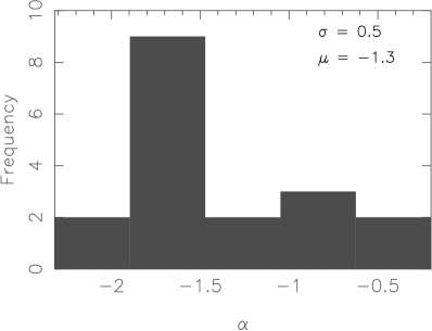
Figure 5: Shaded regions shows the histogram of the distribution of the power law index $\alpha$. Note that the histogram has 5 bins for 18 data points. The sample mean $\mu$ and sample standard deviation $\sigma$ are also shown.

Figure 6: Scatter plot of the average inclination angle $i$ with power law index $\alpha$. The $1-\sigma$ error bars of $\alpha$ is also shown. The value of the linear correlation coefficient $r$ is given at the top right corner.

The galaxies in our sample have a wide range of inclination angles ‘$i$’, ranging from $7^{\circ}$ for NGC 628 to $74^{\circ}$ for NGC 2841. In paper IV we have performed simulations to assess the effect of the inclination angle on power spectrum estimation. We found that though the length scale range over which the power spectrum can be estimated depends on the inclination angles, the power law slope remains constant irrespective of the inclination angle. In order to investigate if the measured slope is influenced by the galaxy’s inclination angle, we have evaluated the linear correlation between the power law index $\alpha$ and the inclination angle of the galaxy ( Figure 6). The lack of correlation (correlation coefficient 0.25) confirms the expectations from the simulations that the dispersion in the values of $\alpha$ is not influenced by the inclination.

It is important to identify the mechanism that generates the large-scale density fluctuations observed in the ISM. Here we consider a few possibilities and try to assess if these mechanisms can give rise to the $\alpha$ values measured in our sample.

Figure 7: Scatter plot of the surface density of the star formation rate (Table 1) with power law index $\alpha$. Open circles show the values from this paper. We also show the same quantities for the five dwarf galaxies from Dutta et al. (2009a) using open boxes. The $1\sigma$ error bars of $\alpha$ are also shown. The left panel shows the SFR per unit area of the optical disk of the galaxies. The right panel shows similar quantities with the surface density of SFR calculated per unit HI disk area. We also evaluate the linear correlation coefficients for each of the two cases using the galaxies in this paper. These values are given at the top right corner of the each panel. The x axis of each plot has a unit of kpc^-2, while the SFR values are considered to be in units of M${}_{\odot}\,$yr^-1.

At small scales, the energy input from star formation processes is a major driving force of the ISM turbulence. Star formation process stir up the ISM and the fluctuations hence generated diffuse to larger scales. If the decay process is scale independent, it can give rise to scale free structures as seen in our study. In such a scenario, the galaxies with higher global star formation rate would have a shallower power spectrum. For a sample of irregular galaxies, Willett et al. (2005) find that on scales of $10-400$ pc the power law index of the H$\alpha$ power spectra becomes steeper as the star formation rate (SFR) per unit area increases. In paper IV we reported a weak correlation between the SFR and the power law index of the H i  intensity fluctuations in dwarf galaxies. To investigate if star formation is driving the turbulence we see here, we calculate the linear correlation coefficient of $\alpha$ with the disk averaged SFR per unit area of the optical disk as well as the SFR per unit area of the H i  disk. The result, shown in Figure 7, suggests that there is no correlation between the SFR and the power law spectral index at the length-scales probed in our study.

ISM turbulence can also be driven by the kinetic energy of the H i  gas. In this case, one would expect the H i  velocity dispersion $\langle\sigma\rangle$ to be correlated with $\alpha$. Tamburro et al. (2009) have estimated $\langle\sigma\rangle$ as well as $\sigma_{25}$ for 11 galaxies in the THINGS sample. We consider here the galaxies with inclination angle smaller than $50^{\circ}$ to reduce the effect of the contribution from large scale velocity gradients in the observed velocity dispersion. These galaxies are listed in Table 3, where columns (2) to (5) give (2) $r_{25}$ in kpc, (3) $\langle\sigma\rangle$ in km s^-1, (4) $\sigma_{25}$ in km s^-1 and (5) $\alpha$. Note that $\sigma_{25}$ represents the velocity dispersion at the radius corresponding to $r_{25}$, within which major star formation takes place, whereas $\langle\sigma\rangle$ is an average over the entire disk. The maximum length scales probed using the power spectrum analysis presented in this paper is comparable to the radius $r_{25}$ for these galaxies, however, the power spectrum estimates are over the entire H i  disk. Figure 9 shows the scatter plot of $\sigma_{25}$ and $\langle\sigma\rangle$ with $\alpha$. We find no correlation between $\alpha$ and $\sigma$ for these six galaxies. Strictly speaking, the velocity dispersion is more likely to be correlated with the amplitude of the power spectrum rather than its slope. Since the estimator that we have used here is not sensitive to the amplitude of the power spectrum, we can not conclusively rule out the influence of the velocity dispersion.

Figure 8: Scatter plot of the dynamical mass $M_{dy}$ and the total HI mass $M_{HI}$ (Table 1) with power law index $\alpha$. The $1-\sigma$ error bars of $\alpha$ is also shown. The value of the linear correlation coefficient $r$ is given at the top right corner.

It is possible that the scale-invariant power-law power spectra measured here may be the outcome of the gravitational effects of the galaxy’s dark matter halo or the self gravity of the galaxy’s H i  gas. In such a scenario, it is possible that $\alpha$ is correlated with the galaxy’s total dynamical mass $M_{dy}$ or its total H i  mass $M_{HI}$. Figure 8 shows a scatter plot of $\alpha$ with $M_{dy}$ (left) and $M_{HI}$ (right) respectively. The dynamical mass estimates are obtained either from the THINGS data (de Blok et al., 2008) whenever available, or from earlier references as discussed in Section 2. The $M_{HI}$ values are taken from Walter et al. (2008). Our analysis yields very low linear correlation coefficients suggesting that the gross gravitational effects of the dark matter halo or the H i  disk are not the responsible for the observed power-law power spectra.

Table 3: The values of $r_{25}$, $\langle\sigma\rangle$, $\sigma_{25}$ for six galaxies of our sample. These values are adopted from Tamburro et al. (2009).

Galname	$r_{25}$	$\langle\sigma\rangle$	$\sigma_{25}$	$\alpha$
	(kpc)	(km s-1)	(km s-1)
NGC 628	$10.1$	$8.0$	$7.7\pm 0.4$	$-1.6\pm 0.1$
NGC 3184	$11.7$	$10.4$	$9.7\pm 0.9$	$-1.3\pm 0.1$
NGC 4736	$5.3$	$12.0$	$12.1\pm 1.4$	$-0.3\pm 0.2$
NGC 5194	$11.4$	$17.7$	$17.0\pm 1.4$	$-1.7\pm 0.2$
NGC 6946	$9.2$	$10.1$	$8.6\pm 0.9$	$-1.6\pm 0.1$
NGC 7793	$5.7$	$11.4$	$9.7\pm 1.1$	$-1.7\pm 0.2$

Figure 9: Scatter plot of $\langle\sigma\rangle$ and $\sigma_{25}$ (Table 3) with power law index $\alpha$.

In summary, the slope $\alpha$ is not correlated with any of the galaxy parameters that we have considered. While $50\%$ of the $\alpha$ values are in the narrow range $-1.9$ to $-1.5$, the remaining galaxies have $\alpha$ values spread over the broad range $-2.2$ to $-0.3$. It is unclear if this large spread arises from statistical fluctuations in the distribution of $\alpha$, or if there is an underlying physical mechanism that is responsible for this.

4 Summary and Conclusion

We have measured the angular power spectrum of 21-cm specific intensity fluctuations for a sample of 18 spiral galaxies drown from THINGS. This is the first comprehensive analysis of the power spectra of a moderately sized sample of external spiral galaxies. For all the galaxies the estimated power spectrum can be well fitted with a single power law across a reasonably large dynamical range. The power-law power spectrum, we find, extends to length-scales as large as $\sim$ 10 kpc indicating the presence of scale-free structures in the ISM on length-scales that are comparable to the size of the galaxy.

In this analysis we have been able to measure the H i  power spectrum over a large range of length-scales spanning from $\sim\ 300$ pc to $\sim\ 16$ kpc across the entire galaxy sample. The power spectra, we find, are well fit by power laws indicating the presence of scale-invariant fluctuations. Fifty percent of the galaxies in our sample have a measured power law index (slope) $\alpha$ in the range $-1.9$ to $-1.5$ (Figure 5). Only one galaxy, NGC 5457, has a slope $\alpha=-2.2$ which is steeper than $-2$. All the other galaxies in our sample have slopes $\alpha\geq-2$.

A large number of earlier studies (summarized in Elmegreen and Scalo 2004), which have probed small length-scales ranging from $~{}10$ pc to $~{}200$ pc, find a power law power spectrum with slope $\alpha\approx-2.8$. This is believed to be the outcome of three dimensional (3D) compressible turbulence in the ISM. If the same process extends to length-scales larger than the galaxy’s scale height, we would expect to see two-dimensional turbulence in the plane of the galaxy’s disc. Dimensional arguments given in Papers II and III lead us to expect the slope of the 2D density fluctuations to be $\alpha\approx-1.8$. This, within estimated measurement errors, is consistent with the slope that we have measured here for most of the galaxies in our sample. This prompts us to believe that the small scales and large scale fluctuations may both originate from the same physical process, presumably turbulence.

Energy input from supernova is believed to be the major driving mechanism for turbulence at small length-scales. However, it is unlikely that this mechanism would be able to generate large scale coherent structures as seen here. Further, the range of length scales that we probe here ranges from $\sim 300$ pc to $~{}16$ kpc which has practically no overlap with the ranges of length scale at which turbulence is believed to be operational in our Galaxy.

Our analysis confirms that the power-law index index has no correlation with inclination angle, SFR, dynamical or total H i  mass of the galaxy. At present we do not have any understanding of the physical process responsible for the scale-invariant large-scale fluctuations measured here. The mass fluctuations in the galaxy’s dark matter halo is an interesting possibility that we plan to pursue in future.

Numerical studies of the magneto-hydrodynamic (MHD) turbulence (Beresnyak et al., 2005; Kowal et al., 2007; Tofflemire et al., 2011; Burkhart and Lazarian, 2012) demonstrate that the Mach number of the medium is correlated with the density fluctuation power spectrum index. Alternatively, the Mach number can also be estimated from the turbulent velocity dispersion of the medium for such MHD turbulence. We are presently investigating possibilities to separate the turbulent velocity dispersion in the H i  gas from it’s thermal counterpart. It may be possible that the H i  column density as well as the velocity dispersion provides measure of similar quantities on the turbulent H i  . However, it is not straightforward to carry over the results of the simulations performed for MHD turbulence to the turbulence in the H i  gas, which may be characteristically different. This can be tested in future studies and give rise to a better understanding of the ISM turbulence in general.

References

- Begum et al. (2006) Begum, A., Chengalur, J.N., Bhardwaj, S., 2006. Power spectrum of HI intensity fluctuations in DDO 210. MNRAS 372, L33–L37. arXiv:astro-ph/0607367.
- Beresnyak et al. (2005) Beresnyak, A., Lazarian, A., Cho, J., 2005. Density Scaling and Anisotropy in Supersonic Magnetohydrodynamic Turbulence. ApJL 624, L93–L96. arXiv:astro-ph/0502547.
- Bigiel et al. (2008) Bigiel, F., Leroy, A., Walter, F., Brinks, E., de Blok, W.J.G., Madore, B., Thornley, M.D., 2008. The Star Formation Law in Nearby Galaxies on Sub-Kpc Scales. AJ 136, 2846–2871. 0810.2541.
- Block et al. (2010) Block, D.L., Puerari, I., Elmegreen, B.G., Bournaud, F., 2010. A Two-component Power Law Covering Nearly Four Orders of Magnitude in the Power Spectrum of Spitzer Far-infrared Emission from the Large Magellanic Cloud. ApJL 718, L1–L6. 1006.2080.
- Bottinelli and Gouguenheim (1973) Bottinelli, L., Gouguenheim, L., 1973. A neutral hydrogen study of the galaxy NGC 5236. AAP 29, 425–429.
- Brunt and Heyer (2002) Brunt, C.M., Heyer, M.H., 2002. Interstellar Turbulence. II. Energy Spectra of Molecular Regions in the Outer Galaxy. ApJ 566, 289–301. arXiv:astro-ph/0110155.
- Burkhart and Lazarian (2012) Burkhart, B., Lazarian, A., 2012. The Column Density Variance-Sonic Mach Number Relationship. ArXiv e-prints 1205.3792.
- Burkhart et al. (2010) Burkhart, B., Stanimirović, S., Lazarian, A., Kowal, G., 2010. Characterizing Magnetohydrodynamic Turbulence in the Small Magellanic Cloud. ApJ 708, 1204–1220. 0911.3652.
- Crovisier and Dickey (1983) Crovisier, J., Dickey, J.M., 1983. The spatial power spectrum of galactic neutral hydrogen from observations of the 21-cm emission line. AAP 122, 282–296.
- de Blok et al. (2008) de Blok, W.J.G., Walter, F., Brinks, E., Trachternach, C., Oh, S., Kennicutt, R.C., 2008. High-Resolution Rotation Curves and Galaxy Mass Models from THINGS. AJ 136, 2648–2719. 0810.2100.
- Deshpande et al. (2000) Deshpande, A.A., Dwarakanath, K.S., Goss, W.M., 2000. Power Spectrum of the Density of Cold Atomic Gas in the Galaxy toward Cassiopeia A and Cygnus A. ApJ 543, 227–234. arXiv:astro-ph/0007366.
- Dutta (2011) Dutta, P., 2011. Probing Turbulence in the Interstellar Medium using Radio-Interferometric Observations of Neutral Hydrogen. ArXiv e-prints 1102.4419.
- Dutta et al. (2008) Dutta, P., Begum, A., Bharadwaj, S., Chengalur, J.N., 2008. HI power spectrum of the spiral galaxy NGC628. MNRAS 384, L34–L37. 0711.1234.
- Dutta et al. (2009a) Dutta, P., Begum, A., Bharadwaj, S., Chengalur, J.N., 2009a. A study of interstellar medium of dwarf galaxies using HI power spectrum analysis. MNRAS 398, 887–897. 0905.1756.
- Dutta et al. (2009b) Dutta, P., Begum, A., Bharadwaj, S., Chengalur, J.N., 2009b. The scaleheight of NGC 1058 measured from its HI power spectrum. MNRAS 397, L60–L63. 0905.1450.
- Dutta et al. (2010) Dutta, P., Begum, A., Bharadwaj, S., Chengalur, J.N., 2010. Turbulence in the harassed galaxy NGC4254. MNRAS 405, L102–L106. 1004.1528.
- Elmegreen et al. (2001) Elmegreen, B.G., Kim, S., Staveley-Smith, L., 2001. A Fractal Analysis of the H I Emission from the Large Magellanic Cloud. ApJ 548, 749–769. arXiv:astro-ph/0010578.
- Elmegreen and Scalo (2004) Elmegreen, B.G., Scalo, J., 2004. Interstellar Turbulence I: Observations and Processes. ARA&A 42, 211–273. arXiv:astro-ph/0404451.
- Green (1993) Green, D.A., 1993. A power spectrum analysis of the angular scale of Galactic neutral hydrogen emission towards L = 140 deg, B = 0 deg. MNRAS 262, 327–342.
- Huchtmeier and Seiradakis (1985) Huchtmeier, W.K., Seiradakis, J.H., 1985. H I observations of galaxies in nearby groups. AAP 143, 216–225.
- Huchtmeier and Witzel (1979) Huchtmeier, W.K., Witzel, A., 1979. Extended envelope of neutral hydrogen around M 101. AAP 74, 138–145.
- Kamphuis and Briggs (1992) Kamphuis, J., Briggs, F., 1992. Kinematics of the extended H I disk of NGC 628 - High velocity gas and deviations from circular rotation. AAP 253, 335–348.
- Kowal et al. (2007) Kowal, G., Lazarian, A., Beresnyak, A., 2007. Density Fluctuations in MHD Turbulence: Spectra, Intermittency, and Topology. ApJ 658, 423–445. arXiv:astro-ph/0608051.
- Lazarian (1995) Lazarian, A., 1995. Study of turbulence in HI using radiointerferometers. AAP 293, 507–520.
- Lazarian and Pogosyan (2000) Lazarian, A., Pogosyan, D., 2000. Velocity Modification of H I Power Spectrum. ApJ 537, 720–748. arXiv:astro-ph/9901241.
- Lazarian and Pogosyan (2004) Lazarian, A., Pogosyan, D., 2004. Velocity Modification of the Power Spectrum from an Absorbing Medium. ApJ 616, 943–965. arXiv:astro-ph/0405461.
- Leroy et al. (2008) Leroy, A.K., Walter, F., Brinks, E., Bigiel, F., de Blok, W.J.G., Madore, B., Thornley, M.D., 2008. The Star Formation Efficiency in Nearby Galaxies: Measuring Where Gas Forms Stars Effectively. AJ 136, 2782–2845. 0810.2556.
- Padoan et al. (2001) Padoan, P., Kim, S., Goodman, A., Staveley-Smith, L., 2001. A New Method to Measure and Map the Gas Scale Height of Disk Galaxies. ApJL 555, L33–L36. arXiv:astro-ph/0103251.
- Roy et al. (2010) Roy, N., Chengalur, J.N., Dutta, P., Bharadwaj, S., 2010. H I 21 cm opacity fluctuations power spectra towards Cassiopeia A. MNRAS 404, L45–L49. 1002.4192.
- Sofue (1996) Sofue, Y., 1996. The Most Completely Sampled Rotation Curves for Galaxies. ApJ 458, 120–+. arXiv:astro-ph/9507098.
- Stanimirovic et al. (1999) Stanimirovic, S., Staveley-Smith, L., Dickey, J.M., Sault, R.J., Snowden, S.L., 1999. The large-scale HI structure of the Small Magellanic Cloud. MNRAS 302, 417–436.
- Tamburro et al. (2009) Tamburro, D., Rix, H., Leroy, A.K., Mac Low, M., Walter, F., Kennicutt, R.C., Brinks, E., de Blok, W.J.G., 2009. What is Driving the H I Velocity Dispersion? AJ 137, 4424–4435. 0903.0183.
- Tofflemire et al. (2011) Tofflemire, B.M., Burkhart, B., Lazarian, A., 2011. Interstellar Sonic and Alfvénic Mach Numbers and the Tsallis Distribution. ApJ 736, 60. 1103.3299.
- Walter et al. (2008) Walter, F., Brinks, E., de Blok, W.J.G., Bigiel, F., Kennicutt, R.C., Thornley, M.D., Leroy, A., 2008. THINGS: The H I Nearby Galaxy Survey. AJ 136, 2563–2647. 0810.2125.
- Willett et al. (2005) Willett, K.W., Elmegreen, B.G., Hunter, D.A., 2005. Power Spectra in V band and H of Nine Irregular Galaxies. AJ 129, 2186–2196. arXiv:astro-ph/0503295.