Hyperbolicity, degeneracy, and expansion of random intersection graphs

Abstract

We establish the conditions under which several algorithmically exploitable structural features hold for random intersection graphs, a natural model for many real-world networks where edges correspond to shared attributes. Specifically, we fully characterize the degeneracy of random intersection graphs, and prove that the model asymptotically almost surely produces graphs with hyperbolicity at least $\log{n}$. Further, we prove that in the parametric regime where random intersection graphs are degenerate an even stronger notion of sparseness, so called bounded expansion, holds with high probability.

We supplement our theoretical findings with experimental evaluations of the relevant statistics.

1 Introduction

There has been a recent surge of interest in analyzing large graphs, stemming from the rise in popularity (and scale) of social networks and significant growth of relational data in science and engineering fields (e.g. gene expressions, cybersecurity logs, and neural connectomes). One significant challenge in the field is the lack of deep understanding of the underlying structure of various classes of real-world networks. Here, we focus on two structural characteristics that can be exploited algorithmically: bounded expansion and hyperbolicity.

A graph class has bounded expansion if, for every member $G$, one cannot form arbitrarily dense graphs by contracting subgraphs of small radius. Formally, the degeneracy of every minor of $G$ is bounded by a function of the depth of that minor (the maximum radius of its branch sets). Bounded expansion offers a structural generalization of both bounded-degree and graphs excluding a (topological) minor. Algorithmically, this property is extremely useful: every first-order-definable problem is decidable in linear fpt-time in these classes [15]. We also consider $\delta$-hyperbolicity, which restricts the structure of shortest-path distances in the graph to be tree-like. Hyperbolicity is closely tied to treelength, but unrelated to measures of structural density such as bounded expansion. Algorithms for graph classes of bounded hyperbolicity often exploit computable approximate distance trees [8] or greedy routing [24]. Both of these properties present challenges for empirical evaluation—bounded expansion is only defined with respect to graph classes (not for single instances), and hyperbolicity is an extremal statistic whose O($n^{4}$) computation is infeasible for many of today’s large data sets. As is typical in the study of network structure, we instead ask how the properties behave with respect to randomized models which are designed to mimic aspects of network formation and structure.

In this paper, we consider the random intersection graph model introduced by Karoński, Scheinerman, and Singer-Cohen [44, 23] which has recently attracted significant attention in the literature [4, 12, 20, 17, 41]. Random intersection graphs are based on the premise that network edges often represent underlying shared interests or attributes. The model first creates a bipartite object-attribute graph $B=(V,A,E)$ by adding edges uniformly at random with a fixed per-edge probability $p(\alpha)$, then considers the intersection graph  $G:=(V,E^{\prime})$, where $xy\in E^{\prime}$ if and only if the neighborhoods of the vertices $x,y$ in $B$ have a non-empty intersection. The parameter $\alpha$ controls both the ratio of attributes to objects and the probability $p$: For $n$ objects, the number of attributes $m$ is proportional to $n^{\alpha}$ and the probability $p$ to $n^{-(1+\alpha)/2}$.

Random intersection graphs are particularly attractive because they meet three important criteria: (1) the generative process makes sense in many real-world contexts, for example collaboration networks of scientists [46, 36]; (2) they are able to generate graphs which match key empirically established properties of real data—namely sparsity, (tunable) clustering and assortativity [12, 3, 4]; and (3) they are relatively mathematically tractable due to significant amounts of independence in the underlying edge creation process. In this paper, we present the following results on the structure of random intersection graphs.

1. For $\alpha\leqslant 1$, with high probability (w.h.p.), random intersection graphs are somewhere dense (and thus do not have bounded expansion) and have unbounded degeneracy.

2. For $\alpha>1$, w.h.p.  random intersection graphs have bounded expansion (and thus constant degeneracy).

3. Under reasonable restrictions on the constants in the model, random intersection graphs have hyperbolicity $\Omega(\log n)$ asymptotically almost surely.

In particular, the second result strengthens the original claim that the model generates sparse graphs for $\alpha>1$, by establishing they are in fact structurally sparse in a robust sense. It is of interest to note that random intersection graphs only exhibit tunable clustering when $\alpha=1$ [12], when our results indicate they are not structurally sparse (in any reasonable sense). Further, we note that the third result is negative—our bound implies a $\log{n}$ lower bound on the treelength [8].

2 Preliminaries

We start with a few necessary definitions and lemmas, covering each of the key ideas in the paper (random intersection graphs, degeneracy, expansion, and hyperbolicity). We use standard notation: $G=(V,E)$ denotes a finite, simple graph on the vertices $V$ with edge set $E$. We alternatively write $V(G)$ and $E(G)$ to denote the edge and vertex set, respectively. For a graph $G$ and a vertex $x\in V(G)$, $N_{G}(x)$ denotes the set of neighbors of $x$ in $G$. A subgraph $H$ of $G$ is induced if for every pair of vertices $u,v\in V(H)$, the edge $(u,v)$ exists in $H$ if and only if it exists in $G$. Paths and cycles consisting of $k$ edges are said to have length $k$ and are denoted $P_{k}$ and $C_{k}$ respectively. For vertices $x$ and $y$ in a graph let $P[x,y]$ denote a shortest path from $x$ to $y$.

We use the terms asymptotically almost surely (a.a.s.) and with high probability (w.h.p.) according to the following conventions: For each integer $n$, let $\mathcal{G}_{n}$ define a distribution on graphs with $n$ vertices (for example, coming from a random graph model). We say the event $E_{n}$ defined on $\mathcal{G}_{n}$ holds asymptotically almost surely (a.a.s.) if $\lim_{n\rightarrow\infty}\mathbb{P}[E_{n}]=1$. We say an event occurs with high probability (w.h.p.) if for any $c\geqslant 1$ the event occurs with probability at least $1-f(c)/n^{c}$ for $n$ greater than some constant, where $f$ is some function only depending on $c$. As a shorthand, we will simply say that $\mathcal{G}_{n}$ has some property a.a.s. (or w.h.p.).

2.1 Random Intersection Graphs

A wide variety of random intersection graph models have been defined in the literature. In this paper, we restrict our attention to the most well-studied of these models, $G(n,m,p)$, which is defined as follows:

Definition 2.1 (Random Intersection Graph Model)

Fix positive constants $\alpha,\beta$ and $\gamma$. Let $B$ be a random bipartite graph on parts of size $n$ and $m=\beta n^{\alpha}$ with each edge present independently with probability $p=\gamma n^{-(1+\alpha)/2}$. Let $V$ (the vertices) denote the part of size $n$ and $A$ (the attributes) the part of size $m$. The associated random intersection graph $G=G(n,m,p)$ is defined on the vertices $V$: two vertices are connected in $G$ if they share (are both adjacent to in $B$) at least one attribute in $A$.

We note that $G(n,m,p)$ defines a distribution $\mathcal{G}_{n}$ on graphs with $n$ vertices. The notation $G=G(n,m,p)$ denotes a graph $G$ that is randomly sampled from the distribution $\mathcal{G}_{n}$. Throughout the manuscript, given a random intersection graph $G(n,m,p)$, we will refer to $B$ as the associated bipartite graph on $n$ vertices and $m$ attributes from which $G$ is formed.

In order to work with graph classes formed by the random intersection graph model, we will need a technical result that bounds the number of attributes in the neighborhood of a subset of vertices around its expected value. These lemmas and their proofs are in Section 2.4.

2.2 Degeneracy & Expansion

Although it is widely accepted that complex networks tend to be sparse (in terms of edge density), this property usually is not sufficient to improve algorithmic tractability: many NP-hard problems on graphs, for instance, remain NP-hard when restricted to graphs with bounded average degree. In contrast, graph classes that are structurally sparse (bounded treewidth, planar, etc.) often admit more efficient algorithms—in particular when viewed through the lens of parameterized complexity. Consequently, we are interested whether random graph models and, by extension, real-world networks exhibit any form of structural sparseness that might be exploitable algorithmically.

As a first step, we would like that a graph is not only sparse on average, but that this property extends to all of its subgraphs. This requirement motivates a very general class of structurally sparse graphs—that of bounded degeneracy.

Definition 2.2 ($k$-core)

The $k$-core of $G$ is the maximum induced subgraph of $G$ in which all vertices have degree at least $k$. The degeneracy of $G$ is the maximum $k$ so that the $k$-core is nonempty (equivalently, the least positive integer $k$ such that every induced subgraph of $G$ contains a vertex with at most $k$ neighbors).

It is easy to see that the degeneracy is lower-bounded by the size of the largest clique. Thus, the degeneracy of intersection graphs is bounded below by the maximum attribute degree in the associated bipartite graph since each attribute contributes a complete subgraph of size equal to its degree to the intersection graph. For certain parameter values, this lower bound will, w.h.p., give the correct order of magnitude of the degeneracy of the graph.

Some classes of graphs with bounded degeneracy have stronger structural properties—here we focus on the so-called graphs of bounded expansion [31]. In the context of networks, bounded expansion captures the idea that networks decompose into small dense structures (e.g. communities) connected by a sparse global structure. More formally, we characterize bounded-expansion classes using special graph minors and an associated density measure ‘grad’ (cf. Figure 1).

Figure 1: The graph $H$ on the right is a $1$-shallow topological minor of $G$, as witnessed by the $\leqslant 2$-subdivision highlighted inside $G$. Further, $H$ is the densest among all $1$-shallow topological minor of $G$: hence $\widetilde{\nabla}\!_{1}(G)=|E(H)|/|V(H)|=9/5$.

Definition 2.3 (Shallow topological minor, nails, subdivision vertices)

A graph $M$ is an $r$-shallow topological minor of $G$ if a $(\leqslant 2r)$-subdivision of $M$ is isomorphic to a subgraph $G^{\prime}$ of $G$. We call $G^{\prime}$ a model of $M$ in $G$. For simplicity, we assume by default that $V(M)\subseteq V(G^{\prime})$ such that the isomorphism between $M$ and $G^{\prime}$ is the identity when restricted to $V(M)$. The vertices $V(M)$ are called nails and the vertices $V(G^{\prime})\setminus V(M)$ subdivision vertices. The set of all $r$-shallow topological minors of a graph $G$ is denoted by $G\mathop{\widetilde{\triangledown}}r$.

Definition 2.4 (Topological grad)

For a graph $G$ and integer $r\geqslant 0$, the topological greatest reduced average density (grad) at depth $r$ is defined as $\widetilde{\nabla}\!_{r}(G)=\max_{H\in G\mathop{\widetilde{\triangledown}}r}|E(H)|/|V(H)|.$ For a graph class $\mathcal{G}$, define $\widetilde{\nabla}\!_{r}(\mathcal{G})=\sup_{G\in\mathcal{G}}\widetilde{\nabla}\!_{r}(G)$.

Definition 2.5 (Bounded expansion)

A graph class $\mathcal{G}$ has bounded expansion if there exists a function $f$ such that for all $r$, we have $\widetilde{\nabla}\!_{r}(\mathcal{G})<f(r)$.

When introduced, bounded expansion was originally defined using an equivalent characterization based on the notion of shallow minors (cf. [31]): $H$ is a $r$-shallow minor of $G$ if $H$ can be obtained from $G$ by contracting disjoint subgraphs of radius at most $r$. In the context of our paper, however, the topological shallow minor variant proves more useful, and we restrict our attention to this setting. Let us point out that bounded expansion implies bounded degeneracy, with $2f(0)$ being an upper bound on the degeneracy of the graphs.

Finally, nowhere dense is a generalization of bounded expansion in which we measure the clique number instead of the edge density of shallow minors. Let $\omega(G)$ denote the size of the largest complete subgraph of a graph $G$ and let $\omega(\mathcal{G})=\sup_{G\in\mathcal{G}}\omega(G)$ be the natural extension to graph classes $\mathcal{G}$.

Definition 2.6 (Nowhere dense [32, 33])

A graph class $\mathcal{G}$ is nowhere dense if there exists a function $f$ such that for all $r\in\mathbf{N}$ it holds that $\omega(\mathcal{G}\mathop{\widetilde{\triangledown}}r)<f(r)$.

See [34] for many equivalent notions. A graph class is somewhere dense precisely when it is not nowhere dense. While in general a graph class with unbounded degeneracy is not necessarily somewhere dense, the negative proofs presented here show that members of the graph class contain w.h.p. large cliques. This simultaneously implies unbounded degeneracy and that the class is somewhere dense (as a clique is a 0-subdivision of itself). Consequently, we prove a clear dichotomy: random intersection graphs are either structurally sparse or somewhere dense.

2.3 Gromov’s Hyperbolicity

The concept of $\delta$-hyperbolicity was introduced by Gromov in the context of geometric group theory [18]. It captures how “tree-like” a graph is in terms of its metric structure, and has received attention in the analysis of real-world networks. We refer the reader to [47, 21, 24, 29], and references therein, for details on the motivating network applications. There has been a recent surge of interest in studying the hyperbolicity of various classes of random networks including small world networks [47, 42], Erdős-Rényi random graphs [30], and random graphs with expected degrees [43].

There are several ways of characterizing $\delta$-hyperbolic metric spaces, all of which are equivalent up to constant factors [7, 8, 18]. Since graphs are naturally geodesic metric spaces when distance is defined using shortest paths, we will use the definition based on $\delta$-slim triangles (originally attributed to Rips [7, 18]).

Definition 2.7 ($\delta$-hyperbolicity)

A graph $G=(V,E)$ is $\delta$-hyperbolic if for all $x,y,z\in V$, for every choice of geodesic (shortest) paths between them— denoted $P[x,y],P[x,z],P[y,z]$—we have $\forall v\in P[x,y],\;\exists w\in P[x,z]\cup P[z,y]:\;d_{G}(v,w)\leqslant\delta,$ where $d_{G}(v,w)$ is shortest-path distance of $v$ to $w$ in $G$.

That is, if $G$ is $\delta$-hyperbolic, then for each triple of vertices $x,y,z$, and every choice of three shortest paths connecting them pairwise, each point on the shortest path from $x$ to $y$ must be within distance $\delta$ of a point on one of the other paths. The hyperbolicity of a graph $G$ is the minimum $\delta\geqslant 0$ so that $G$ is $\delta$-hyperbolic. Note that a trivial upper bound on the hyperbolicity is half the diameter (this is true for any graph).

In this paper we give lower bounds for the hyperbolicity of the graphs in $G(n,m,p)$. We believe these bounds are asymptotically the correct order of magnitude (e.g. also upper bounds). This would require that the the diameter of connected components is also logarithmic in $n$, which has been shown for a similar model [40].

2.4 Concentration Results for Neighborhood Unions

This section states and proves results showing that in random intersection graphs the number of attributes in the combined neighborhood of a subset of vertices is tightly concentrated around its expected value when $\alpha>1$, and has a tight lower bound when $\alpha=1$ and the subset under consideration is large enough.

Lemma 1

Let $\alpha>1$ and fix $\epsilon>0$. Then if $G(n,m,p)$ is a random intersection graph on vertex set $V$ and $S\subset V$, w.h.p. $(1-\epsilon)|S|mp\leqslant|N_{B}(S)|\leqslant(1+\epsilon)|S|mp.$

Proof

Let $\epsilon>0$. Let $v$ be a vertex in $G$ and let $A(v)$ denote the number of attributes adjacent to $v$ in the associated bipartite graph $B$. Since each attribute is adjacent to $v$ independently with probability $p$, $A(v)$ has a binomial distribution and by Bernstein’s inequality:

$$\mathbb{P}[A(v)>(1+\epsilon)mp]\leqslant\exp-\Big{(}\frac{\epsilon^{2}mp}{2(1+\epsilon/3)}\Big{)}=o\Big{(}\frac{1}{n^{c}}\Big{)}$$

for any fixed $c.$ By the union bound, it follows that with high probability $|N_{B}(S)|\leqslant(1+\epsilon)|S|mp$.

For each attribute $a$ in $B$, let $\mathcal{I}_{a}$ be the indicator random variable equal to $1$ when $a$ has at least one neighbor in $S$. Since these variables are independently and identically distributed, we again use Bernstein’s inequality:

$$\mathbb{P}\big{[}\textstyle\sum_{a}\mathcal{I}_{a}<(1-\epsilon)m\mathbb{P}[\mathcal{I}_{a}=1]\big{]} \leqslant\exp-\Big{(}\frac{\epsilon^{2}m\mathbb{P}[\mathcal{I}_{a}]}{2}\Big{)}$$

$$\leqslant\exp-\Big{(}\frac{\epsilon^{2}m(1-\epsilon)|S|p}{2}\Big{)}$$

$$\leqslant o\Big{(}\frac{1}{n^{c}}\Big{)}$$

for any fixed $c$. The penultimate inequality follows from

$$\mathbb{P}[\mathcal{I}_{a}=1]=1-(1-p)^{|S|}\geqslant|S|p(1-o(1)).$$

∎

Lemma 2

Let $\alpha=1$ and fix $\eta,\epsilon>0$. If $G(n,m,p)$ is a random intersection graph on vertex set $V$ and $S\subset V$ a subset of size at least $\eta n$, then w.h.p. it holds that $|N_{B}(S)|\geqslant(1-\epsilon)|S|mp.$

Proof

Again, for each attribute $a$ in $B$, let $\mathcal{I}_{a}$ be the indicator random variable equal to $1$ when $a$ has at least one neighbor in $S$.

$$\mathbb{P}\big{[}\textstyle\sum_{a}\mathcal{I}_{a}<(1-\epsilon)m\mathbb{P}[\mathcal{I}_{a}=1]\big{]} \leqslant\exp-\Big{(}\frac{\epsilon^{2}m\mathbb{P}[\mathcal{I}_{a}]}{2}\Big{)}$$ (1)

$$\leqslant\exp-\Big{(}\frac{\epsilon^{2}m\left(1-e^{p|S|}\right)}{2}\Big{)}$$ (2)

$$\leqslant o\Big{(}\frac{1}{n^{c}}\Big{)}$$ (3)

for any fixed $c$. Again we use the fact that $\mathbb{P}[\mathcal{I}_{a}=1]=1-(1-p)^{|S|}\geqslant 1-e^{p|S|}.$ ∎

3 Structural sparsity of random intersection graphs

In this section we will characterize a clear break in the sparsity of graphs generated by $G(n,m,p)$, depending on whether $\alpha$ is strictly greater than one. In each case, we analyze (probabilistically) the degeneracy and expansion of the generated class.

Theorem 3.1

Fix constants $\alpha,\beta$ and $\gamma$. Let $m=\beta n^{\alpha}$ and $p=\gamma n^{-(1+\alpha)/2}$. Let $G=G(n,m,p)$. Then the following hold w.h.p.

1. If $\alpha<1$, $G(n,m,p)$ is somewhere dense and $G$ has degeneracy $\Omega(\gamma n^{(1-\alpha)/2})$.

2. If $\alpha=1$, $G(n,m,p)$ is somewhere dense and $G$ has degeneracy $\Omega(\frac{\log n}{\log\log n})$.

3. If $\alpha>1$, $G(n,m,p)$ has bounded expansion and thus $G$ has degeneracy $O(1)$.

We prove each of the three cases of Theorem 3.1 separately.

3.1 Proof of Theorem 3.1 when $\alpha\leqslant 1$

When $\alpha\leqslant 1$, we prove that w.h.p. the random intersection graph model generates graph classes with unbounded degeneracy by establishing the existence of a high-degree attribute in the associated bipartite graph (thus lower-bounding the clique number). The proof is divided into two lemmas, one for $\alpha<1$ and one for $\alpha=1$, in which we prove different lower bounds.

Lemma 3

Fix constants $\alpha<1,\beta$ and $\gamma$. If $m=\beta n^{\alpha}$ and $p=\gamma n^{-(1+\alpha)/2}$, then w.h.p. $G=G(n,m,p)$ has degeneracy $\Omega(\gamma n^{(1-\alpha)/2}$).

Proof

Let $G=G(n,m,p)$ and $B=(V,A,E)$ be the bipartite graph associated with $G$. Define the random variable $X_{i}$ to be the number of vertices in $V$ connected to a particular attribute $a_{i}$. Then $X_{i}\sim Binom(n,p)$ and $\mathbb{P}[X_{i}<np-1]\leqslant 1/2$, since the median of $X_{i}$ lies between $\lfloor np\rfloor$ and $\lceil np\rceil$. Let $\mathcal{S}$ be the event that $|X_{i}|<np-1$ for all $i\in[1,m]$. Since the number of vertices attached to each attribute is independent,

$$\mathbb{P}[\mathcal{S}]=\prod_{i=1}^{m}\left(1-\mathbb{P}[X_{i}\geqslant np-1]\right)\leqslant\left[1-(1-1/2)\right]^{m}=2^{-m}.$$

Now, it follows that $\lim_{n\rightarrow\infty}\mathbb{P}[\mathcal{S}]=0$, and w.h.p. the graph $G$ contains a clique of size $np-1=\gamma n^{(1-\alpha)/2}-1$, and thus has degeneracy at least $np-1$. ∎

Corollary 1

Fix constants $\alpha<1,\beta$ and $\gamma$. If $m=\beta n^{\alpha}$ and $p=\gamma n^{-(1+\alpha)/2}$, then w.h.p. $G(n,m,p)$ is somewhere dense.

Proof

The proof of Lemma 3 shows that w.h.p. a clique of size $\gamma n^{(1-\alpha)/2}$ exists already as a subgraph (i.e. a $0$-subdivision) in every $G\in G(n,m,p)$. ∎

The following lemma addresses the case when the attributes grow at the same rate as the number of vertices. We note that Bloznelis and Kurauskas independently proved a similar result (using a slightly different RIG model) in [5]; we include a slightly more direct proof here for completeness.

Lemma 4

Fix constants $\alpha=1,\beta$ and $\gamma$. Then a random graph $G=G(n,m,p)$ has degeneracy $\Omega(\frac{\log n}{\log\log n})$ w.h.p.

Proof

Let $c$ be any constant greater than one. We will show that for every $k\leqslant\frac{\log n}{\log\log n}$, a random graph $G\in G(n,m,p)$ contains a clique of size $k$ with probability at least $\Omega(1-n^{-c})$. Fix an attribute $a$. The probability that $a$ has degree at least $k$ in the bipartite graph is at least the probability that it is exactly $k$, hence

$${n\choose k}p^{k}(1-p)^{n-k}\geqslant{n\choose k}p^{k}(1-p)^{n}\geqslant\frac{\gamma^{k}}{e^{\gamma}k^{k}}.$$

We will show that this converges fast enough for $\gamma<1$; the case for $\gamma\geqslant 1$ works analogously. Therefore the probability that none of the $m=\beta n$ attributes has degree at least $k$ is at most

$$\left(1-\frac{\gamma^{k}}{e^{\gamma}k^{k}}\right)^{\beta n}\leqslant e^{-\beta n\left(\frac{\gamma^{k}}{e^{\gamma}k^{k}}\right)}.$$

We prove that this probability is smaller than $n^{-c}$ by showing that

$$\frac{\beta}{e^{\gamma}}\frac{n\gamma^{k}}{k^{k}}\geqslant c\cdot\log n,$$ (4)

when $k=\frac{\log n}{\log\log n}$. Let $c^{\prime}=ce^{\gamma}/\beta$. Then to show Inequality 4 holds, it is enough to show

$$n\frac{(\gamma\log\log n)^{\log n/\log\log n}}{(\log n)^{\log n/\log\log n}}=(\gamma\log\log n)^{\frac{\log n}{\log\log n}}\geqslant c^{\prime}\cdot\log n.$$

Comparing the functions $e^{x/\log x}$ and $c^{\prime}x$, we see that for large enough positive $x$,

$$x>\log c^{\prime}\log x+\log^{2}x$$

and equivalently

$$e^{x/\log x}>c^{\prime}\cdot x.$$

Therefore for large enough $n$, $e^{\log n/\log\log n}>c^{\prime}\cdot\log n$, and in particular, for $n>e^{e^{e/\gamma}}$,

$$(\gamma\log\log n)^{\frac{\log n}{\log\log n}}\geqslant c^{\prime}\cdot\log n,$$

as previously claimed. This shows the probability that no attribute has degree at least $\log n/\log\log n$ is at most $O(n^{-c})$, and the claim follows. ∎

Corollary 2

Fix constants $\alpha=1,\beta$ and $\gamma$. If $m=\beta n^{\alpha}$ and $p=\gamma n^{-(1+\alpha)/2}$, then w.h.p. $G(n,m,p)$ is somewhere dense.

Proof

Lemma 4 is proven by showing that w.h.p. it holds that a clique of size $\Omega\left(\log n/(\log\log n)\right)$ exists as a subgraph (i.e. a $0$-subdivision) in every graph in $G(n,m,p)$. ∎

3.2 Proof of Theorem 3.1 when $\alpha>1$

In this section, we focus on the case when $\alpha>1$. This is the parameter range in which the model generates sparse graphs.

Before beginning, we note that if $G(n,m,p)$ has bounded expansion w.h.p., then for any $p^{\prime}\leqslant p$ and $m^{\prime}\leqslant m$ it follows that w.h.p. $G(n,m^{\prime},p^{\prime})$ also has bounded expansion by a simple coupling argument. Thus we can assume without loss of generality that both $\gamma$ and $\beta$ are greater than one. For the remainder of this section, we fix the parameters $\gamma,\beta,\alpha>1$, the resulting number of attributes $m=\beta n^{\alpha}$ and the per-edge probability $p=\gamma n^{-(1+\alpha)/2}$.

3.2.1 Bounded Attribute-Degrees

As mentioned before, for a random intersection graph to be degenerate, the attributes of the associated bipartite graph must have bounded degree. We prove that w.h.p., this necessary condition is satisfied.

Lemma 5

Let $c\geqslant 1$ be a constant such that $2\frac{\alpha+c}{\alpha-1}>\beta\gamma e$. Then the probability that there exists an attribute in the bipartite graph associated with $G(n,m,p)$ of degree higher than $2\frac{\alpha+c}{\alpha-1}$ is $O(n^{-c})$.

Proof

Taking the union bound, the probability that some attribute has degree larger than $d$ is upper bounded by

$$m{n\choose d}p^{d} \leqslant\frac{\beta e^{d}\gamma^{d}}{d^{d}}\cdot\frac{n^{\alpha+d}}{n^{\frac{a+1}{2}d}},$$

where the first fraction is bounded by a constant as soon as $d>e\beta\gamma$. Then we achieve an upper bound of $O(n^{-c})$ as soon as $\frac{\alpha+1}{2}d-d-\alpha>c$, or equivalently, $d>2\frac{\alpha+c}{\alpha-1}$, proving the claim. ∎

This result allows us to assume for the remainder of the proof that the maximum attribute degree is bounded.

3.2.2 Alternative Characterization of Bounded Expansion

We now state a characterization of bounded expansion which is often helpful in establishing the property for classes formed by random graph models.

Proposition 1 (​[35, 34])

A class $\cal C$ of graphs has bounded expansion if and only if there exists real-valued functions $f_{1},f_{2},f_{3},f_{4}\colon\mathbf{R}\rightarrow\mathbf{R}^{+}$ such that the following two conditions hold:

1. For all positive $\epsilon$ and for all graphs $G\in\cal C$ with $|V(G)|>f_{1}(\epsilon)$, it holds that $\frac{1}{|V(G)|}\cdot|\{v\in V(G)\colon\deg(v)\geqslant f_{2}(\epsilon)\}|\leqslant\epsilon.$

2. For all $r\in\mathbf{N}$ and for all $H\subseteq G\in\cal C$ with $\widetilde{\nabla}\!_{r}(H)>f_{3}(r)$, it follows that

   $$|V(H)|\geqslant f_{4}(r)\cdot|V(G)|.$$

Intuitively, this result states that any class of graphs with bounded expansion is characterized by two properties:

1. All sufficiently large members of the class have a small fraction of vertices of large degree.

2. All subgraphs of $G\in\cal C$ whose shallow topological minors are sufficiently dense must necessarily span a large fraction of the vertices of $G$.

3.2.3 Stable $r$-Subdivisions

In order to disprove the existence of an $r$-shallow topological minor of a certain density $\delta$, we introduce a stronger topological structure.

Definition 3.2 (Stable $r$-subdivision)

Given graphs $G,H$ we say that $G$ contains $H$ as a stable $r$-subdivision if $G$ contains $H$ as a $\frac{r}{2}$-shallow topological minor with model $G^{\prime}$ such that every path in $G^{\prime}$ corresponding to an edge in $H$ has exactly length $r+1$ and is an induced path in $G$.

A stable $r$-subdivision is by definition a shallow topological minor, thus the existence of an $r$-subdivision of density $\delta$ implies that $\widetilde{\nabla}\!_{\frac{r}{2}}(G)\geqslant\delta$. We prove that the densities are also related in the other direction.

Lemma 6

A graph $G$ with $\widetilde{\nabla}\!_{\frac{r}{2}}(G)\geqslant\delta$ contains a stable $i$-subdivision of density at least $\delta/(r+1)$ for some $i\in\{0,\dots,r\}$.

Proof

Consider a $\frac{r}{2}$-shallow topological minor $H$ of $G$ with density at least $\delta$. Let $H^{\prime}\subseteq G$ be the model of $H$ and let $\lambda\colon V(H^{\prime})\to V(H)\cup E(H)$ be a mapping that maps nails of the model to vertices of the minor and subdivision vertices of the model to their respective edge in the model. Consider the preimage $\lambda^{-1}$. As a slight abuse of notation, we can consider $\lambda^{-1}$ as a map to (possibly empty) paths of $H$: indeed, we can assume that every edge of $H$ is mapped by $\lambda^{-1}$ to an induced path in $H^{\prime}$. If $H^{\prime}$ uses any non-induced paths, we can replace each such path by a (shorter) induced path and obtain a (different) model of $H$ with the desired property.

We partition the edges of $H$ by the length of their respective paths in the model: define $E_{\ell}=\{e\in H\mid|\lambda^{-1}(e)|=\ell\}$ for $0\leqslant\ell\leqslant r+1$. Since $|E(H)|=\bigcup_{0\leqslant\ell\leqslant r+1}|E_{\ell}|\geqslant\delta|V(H)|$, there exists at least one set $E_{\ell}$ such that $|E_{\ell}|\geqslant\delta|V(H)|/(r+1)$. Then the subgraph $(V(H),E_{\ell})$ is a stable $\ell$-subdivision of $G$. ∎

To show that a graph has no $r$-shallow minor of density $\delta$, it now suffices to prove that no stable $i$-subdivision of density $\delta/(2r+1)$ exists for any $i\in\{0,\dots,2r\}$. We note that the other direction would not work, since the existence of a stable $i$-subdivision for some $i\in\{0,\dots,2r\}$ of density $\delta/(2r+1)$ does not imply the existence of an $r$-shallow topological minor of density $\delta$.

We now establish the probability of having this structure in the random intersection graph model, noting that the following structural result is surprisingly useful, and appears to have promising applications beyond this work. We will argue that a dense subdivision in $G$ implies the existence of a dense subgraph in the associated bipartite graph. We show this claim by considering the existence of a stable $r$-subdivision where all paths are induced, which is generated by a minimal number of attributes. Notice that if a model of some graph $H$ exists, then so does a model with these properties. This fact allows us to only consider attributes with minimum degree two, since every edge in the path is generated by a different attribute. This assumption is key in proving the following theorem.

Theorem 3.3

Let $c\geqslant 1$ be a constant and let $\phi=(6eg\beta\gamma r\delta)^{5r\delta 2/(\alpha-1)}$. The probability that $G(n,m,p)$ contains a stable $r$-subdivision with $k$ nails for $r\geqslant 1$ and of density $\delta>1$ is at most

$$r\delta k\cdot\left(\frac{\phi}{n}\right)^{\frac{\alpha-1}{2}k}$$

Proof

Let us first bound the probability that the bipartite graph associated with $G=G(n,m,p)$ contains a dense subgraph. We will then argue that a dense subdivision in $G$ implies the existence of such a dense bipartite subgraph.

Let $\mathbb{P}_{\text{dense}}(\kappa,\nu,\lambda)$ be the probability that there exists sets $V^{\prime}\subseteq V$, $A^{\prime}\subseteq A$, of size $\kappa$ and $\nu$ respectively, such that there exist at least $\lambda$ edges between vertices of $V^{\prime}$ and $A^{\prime}$. It is easy to see that this probability is bounded by

$$\mathbb{P}_{\text{dense}}(\kappa,\nu,\lambda) \leqslant\binom{n}{\kappa}\binom{m}{\nu}\sum_{d_{1},\dots,d_{\nu}}\prod_{i=1}^{\nu}\binom{\kappa}{d_{i}}p^{d_{i}},$$ (5)

where $d_{1},\dots,d_{\nu}$ represent all possible choices of the degrees of $\nu$ attributes such that $\sum_{i=1}^{\nu}{d_{i}}=\lambda$. By Lemma 5, w.h.p. $d_{i}\leqslant g$ and thus w.h.p. there are at most $g^{\nu}$ terms in the sum of (5). Using this together with Stirling’s approximation allows us to simplify the bound as follows:

$$\mathbb{P}_{\text{dense}}(\kappa,\nu,\lambda)\leqslant\left(\frac{ne}{\kappa}\right)^{\kappa}\left(\frac{gme}{\nu}\right)^{\nu}\left(\kappa ep\right)^{\lambda}=\frac{e^{\kappa+\nu+\lambda}g^{\nu}\beta^{\nu}\gamma^{\lambda}}{\nu^{\nu}}\frac{\kappa^{\lambda}n^{\alpha\nu+\kappa}}{\kappa^{\kappa}n^{\frac{\alpha+1}{2}\lambda}}.$$ (6)

Consider a stable $r$-subdivision $H$ in $G$ with $k$ nails and density $\delta$. The model of $H$ uses exactly $k+r\delta k$ vertices of $G$. Let $A_{H}$ be a minimal set of attributes that generates the edges of the model of $H$ in $G$. There is at least one edge between every nail and an attribute in $A_{H}$. Furthermore, since the paths connecting the nails in the model are induced, every subdivision vertex has at least two edges to the attributes $A_{H}$. We conclude that there exists a bipartite subgraph with $\kappa=k+r\delta k$ and $\lambda=2r\delta k+k$. Since $A_{H}$ is minimal, every attribute of $A_{H}$ generates at least one edge in the model of $H$ and therefore $|A_{H}|\leqslant(r+1)\delta k$. Let $\delta_{1}=(r\delta+1)$ and $\delta_{2}=(2r\delta+1)$. By the bound in Equation 6, the probability of such a structure is at most

$$\sum_{\nu=r\delta k/g}^{r\delta k}\mathbb{P}_{\text{dense}}(\delta_{1}k,\nu,\delta_{2}k)$$

$$\leqslant~{} \sum_{\nu=r\delta k/g}^{r\delta k}\frac{e^{{\delta_{1}k}+\nu+{\delta_{2}k}}g^{\nu}\beta^{\nu}\gamma^{{\delta_{2}k}}}{\nu^{\nu}{(\delta_{2}k)}^{{\delta_{2}k}}}\frac{{(\delta_{1}k)}^{{\delta_{2}k}}n^{\alpha\nu+\delta_{1}k}}{{(\delta_{1}k)}^{{\delta_{1}k}}n^{\frac{\alpha+1}{2}{\delta_{2}k}}}$$

Let $\psi$ be the exponent of $1/n$ in a term of this sum. Then we have

$$\psi =\left(\left(\frac{\alpha+1}{2}\right){\delta_{2}k}-(\alpha\nu+\delta_{1}k)\right)$$

$$=\left(\left(\frac{\alpha+1}{2}\right){(2r\delta+1)k}-(\alpha\nu+(r\delta+1)k)\right).$$

Simplifying, we see that

$$\psi=(\alpha+1)r\delta k+\frac{\alpha+2}{2}k-\alpha\nu-(r\delta+1)k=\frac{\alpha-1}{2}k+\alpha(r\delta k-\nu).$$

Thus we can rewrite the previous inequality as

$$\sum_{\nu=r\delta k/g}^{r\delta k}\mathbb{P}_{\text{dense}}(\delta_{1}k,\nu,\delta_{2}k)$$

$$\leqslant{} \sum_{\nu=r\delta k/g}^{r\delta k}\frac{e^{{\delta_{1}k}+\nu+{\delta_{2}k}}g^{\nu}\beta^{\nu}\gamma^{{\delta_{2}k}}{\delta_{1}}^{{\delta_{2}k}}}{{\delta_{1}}^{{\delta_{1}k}}}\frac{{k}^{{\delta_{2}k}}}{\nu^{\nu}{k}^{{\delta_{1}k}}n^{\alpha(r\delta k-\nu)}}\frac{1}{n^{\frac{\alpha-1}{2}k}}$$

$$\leqslant{} \left(\frac{e^{{\delta_{1}}+{r\delta}+{\delta_{2}}}g^{r\delta}\beta^{r\delta}\gamma^{{\delta_{2}}}{\delta_{1}}^{{\delta_{2}}}}{{\delta_{1}}^{{\delta_{1}}}}\right)^{k}\sum_{\nu=r\delta k/g}^{r\delta k}\frac{{k}^{{\delta_{2}k}}}{\nu^{\nu}{k}^{{\delta_{1}k}}n^{\alpha(r\delta k-\nu)}}\frac{1}{n^{\frac{\alpha-1}{2}k}}$$

$$\leqslant{} \left(\frac{e^{{\delta_{1}}+{r\delta}+{\delta_{2}}}g^{2r\delta}\beta^{r\delta}\gamma^{{\delta_{2}}}{\delta_{1}}^{{\delta_{2}}}}{{\delta_{1}}^{{\delta_{1}}}}\right)^{k}\sum_{\nu=r\delta k/g}^{r\delta k}\frac{{k}^{{\delta_{2}k}}}{(r\delta k)^{\nu}{k}^{{\delta_{1}k}}k^{\alpha(r\delta k-\nu)}}\frac{1}{n^{\frac{\alpha-1}{2}k}}$$

$$\leqslant{} \left(e^{{\delta_{1}}+{r\delta}+{\delta_{2}}}g^{2r\delta}\beta^{r\delta}\gamma^{{\delta_{2}}}{\delta_{1}}^{{\delta_{2}}}\right)^{k}\sum_{\nu=r\delta k/g}^{r\delta k}\frac{{k}^{{\delta_{2}k}}}{k^{\nu}{k}^{{\delta_{1}k}}k^{\alpha(r\delta k-\nu)}}\frac{1}{n^{\frac{\alpha-1}{2}k}}$$

Let $\psi^{\prime}$ be the exponent of $k$ in a term of this sum. Then we have

$$\psi^{\prime} =\delta_{2}k-\nu-\delta_{1}k-\alpha(r\delta k)+\alpha\nu$$

$$=(1-\alpha)(r\delta k)+(\alpha-1)\nu$$

$$\leqslant 0.$$

Using $\phi$ as defined, we arrive at the following inequality:

$$\sum_{\nu=r\delta k/g}^{r\delta k}\mathbb{P}_{\text{dense}}(\delta_{1}k,\nu,\delta_{2}k)\leqslant\phi^{\frac{(\alpha-1)}{2}k}\sum_{\nu=r\delta k/g}^{r\delta k}\frac{1}{n^{\frac{\alpha-1}{2}k}}\leqslant{}r\delta k\cdot\left(\frac{\phi}{n}\right)^{\frac{\alpha-1}{2}k}$$ (7)

This inequality completes our proof. ∎

3.2.4 Density

Before turning to our main result, we need two more lemmas that establish the probability of graphs generated using $G(n,m,p)$ having special types of dense subgraphs.

Theorem 3.4

Let $c\geqslant 1$ be a constant and let $g:=2\frac{\alpha+c}{\alpha-1}$. For $u\leqslant m,k\leqslant n$, the probability that the bipartite graph associated with $G(n,m,p)$ contains $u$ attributes of degree $\leqslant g$ that generate at least $\rho\geqslant u$ edges between $k$ fixed vertices is at most

$$\left(\frac{e^{g+1}\gamma^{g}g\beta}{u/k}\right)^{u}\left(\frac{k}{n}\right)^{u}.$$

We note that it is perhaps surprising that $\rho$ disappears in the upper bound given above. Since we are assuming that the degree of the attributes is bounded by $g$, the number of attributes $u$ must be at least $\rho/{g\choose 2}$. Thus the $\rho$ reappears upon expansion. Since we can bound the degree of the attributes w.h.p. when $\alpha>1$, this theorem is generally applicable to sparse random intersection graphs.

Proof

The probability that $u$ attributes of maximal degree $g$ generate at least $\rho\geqslant u$ edges between $k$ fixed vertices can be upper-bounded by

$${m\choose u}\sum_{d_{1},\dots,d_{u}}\prod_{i=1}^{u}{k\choose d_{i}}p^{d_{i}},$$

where $d_{1},\dots,d_{u}$ represent all possible choices of the degrees of $u$ attributes such that $\sum_{i=1}^{u}{d_{i}\choose 2}\geqslant\rho$ (i.e. the degrees of the chosen attributes can generate enough edges). Let $D=\sum_{i=1}^{u}d_{i}$. From Stirling’s inequality, it follows that

$${m\choose u}\sum_{d_{1},\dots,d_{u}}\prod_{i=1}^{u}{k\choose d_{i}}p^{d_{i}}\leqslant ~{}\frac{(e\beta n^{\alpha})^{u}}{u^{u}}\sum_{d_{1},\dots,d_{u}}\prod_{i=1}^{u}\frac{(ek)^{d_{i}}}{d_{i}^{d_{i}}}\left(\frac{\gamma}{n^{(\alpha+1)/2}}\right)^{d_{i}}$$

$$= ~{}\frac{(e\beta)^{u}n^{\alpha u}}{u^{u}}\sum_{d_{1},\dots,d_{u}}\frac{e^{D}k^{D}}{\prod_{i=1}^{u}d_{i}^{d_{i}}}\frac{\gamma^{D}}{n^{\frac{\alpha+1}{2}D}}$$

$$\leqslant ~{}\frac{(e\beta)^{u}(e\gamma)^{gu}n^{\alpha u}}{u^{u}}\sum_{d_{1},\dots,d_{u}}\frac{k^{D}}{n^{\frac{\alpha+1}{2}D}}.$$

Since each $d_{i}$ is at most $g$, we can upper bound this term by

$${m\choose u}\sum_{d_{1},\dots,d_{u}}\prod_{i=1}^{u}{k\choose d_{i}}p^{d_{i}} \leqslant\frac{(e^{g+1}\gamma^{g}\beta)^{u}n^{\alpha u}}{u^{u}}\cdot\sum_{d_{1},\dots,d_{u}}\frac{k^{D}}{n^{\frac{\alpha+1}{2}D}}$$

$$=\left(\frac{e^{g+1}\gamma^{g}\beta}{u/k}\right)^{u}\sum_{d_{1},\dots,d_{u}}\frac{n^{\alpha u}k^{D-u}}{n^{\frac{\alpha+1}{2}D}}.$$

We want to show that $(n^{\alpha u}k^{D-u})/(n^{\frac{\alpha+1}{2}D})$ is bounded by $(k/n)^{x}$ for some $x\geqslant u$. Let us first look at the following inequality:

$$\left(\frac{\alpha+1}{2}\right)D-\alpha u\geqslant D-u\Leftrightarrow D\geqslant 2u$$

Notice that an attribute of degree one generates no edges, thus we can assume that all $d_{i}\geqslant 2$. It follows that $D\geqslant 2u$ and thus the inequality holds, therefore

$$(n^{\alpha u}k^{D-u})/(n^{\frac{\alpha+1}{2}D})\leqslant\left(\frac{k}{n}\right)^{D-u}\leqslant\left(\frac{k}{n}\right)^{u}.$$

The probability of $u$ attributes generating at least $\rho$ edges between $k$ vertices is then at most

$${m\choose u}\sum_{d_{1},\dots,d_{u}}{k\choose d_{i}}p^{d_{i}}\leqslant\left(\frac{e^{g+1}\gamma^{g}\beta}{u/k}\right)^{u}\sum_{d_{1},\dots,d_{u}}\left(\frac{k}{n}\right)^{u}.$$

Finally, since any $d_{i}$ can be at most $g$, we can get rid of the sum by multiplying with a $g^{u}$ factor:

$$\left(\frac{e^{g+1}\gamma^{g}\beta}{u/k}\right)^{u}\sum_{d_{1},\dots,d_{u}}\left(\frac{k}{n}\right)^{u}\leqslant\left(\frac{e^{g+1}\gamma^{g}g\beta}{u/k}\right)^{u}\left(\frac{k}{n}\right)^{u}.$$

∎

The following lemma is a rather straightforward consequence of Theorem 3.4.

Lemma 7

Let $c\geqslant 1$ be a constant, $g:=2\frac{\alpha+c}{\alpha-1}$, $g^{\prime}:={g\choose 2}$ and $\delta>e^{g+1}\gamma^{g}gg^{\prime}\beta$. Then the probability that $G(n,m,p)$ contains a subgraph of density $\delta$ on $k$ vertices is at most

$$\delta k\left(\frac{k}{n}\right)^{\frac{\delta k}{g^{\prime}}}.$$

Proof

By Lemma 5 we can disregard all graphs whose associated bipartite graphs have an attribute of degree greater than $g$. We can bound the probability with:

$$\sum_{u=\frac{\delta k}{g^{\prime}}}^{\delta k}{m\choose u}\sum_{d_{1},\dots,d_{u}}{k\choose d_{i}}p^{d_{i}},$$ (8)

where $d_{1},\dots,d_{u}$ represent the degrees of the $u$ attributes such $\sum_{i=1}^{u}{d_{i}\choose 2}\geqslant\delta k$ (i.e. the degrees of the $u$ attributes that generate all direct edges).

Using Theorem 3.4, the right hand side of Equation 8 is bounded by

$$\sum_{u=\frac{\delta k}{g^{\prime}}}^{\delta k}\left(\frac{e^{g+1}\gamma^{g}g\beta}{u/k}\right)^{u}\left(\frac{k}{n}\right)^{u} \leqslant{}\sum_{u=\frac{\delta k}{g^{\prime}}}^{\delta k}\left(\frac{e^{g+1}\gamma^{g}gg^{\prime}\beta}{\delta}\right)^{u}\left(\frac{k}{n}\right)^{u},$$

using the fact that $u/k\geqslant\delta/g^{\prime}$. Since we set up $\delta\geqslant e^{g+1}\gamma^{g}gg^{\prime}\beta$, we can cancel these terms and simplify the above to

$$\mathbb{P}_{\text{direct}}\leqslant{}\sum_{u=\frac{\delta k}{g^{\prime}}}^{\delta k}\left(\frac{k}{n}\right)^{u}\leqslant\delta k\left(\frac{k}{n}\right)^{\frac{\delta k}{g^{\prime}}},$$

using the fact that $k/n$ is smaller than one. ∎

3.2.5 Main Result

We finally have all the necessary tools to prove the main theorem of this section.

Theorem 3.5

Fix positive constants $\alpha>1$, $\beta$ and $\gamma$. Then w.h.p. the class of random intersection graphs $G(n,m,p)$ defined by these constants has bounded expansion.

Proof

We show the two conditions of Proposition 1 are satisfied in Lemma 8 and Lemma 9, respectively.∎

Lemma 8

Let $c\geqslant 1$ be a constant, $g:=2\frac{\alpha+c}{\alpha-1}$ $g^{\prime}:={g\choose 2}$, and $\lambda$ be a constant bigger than $\max(2e^{g+2}\gamma^{g}g\beta,~{}c)$. For $G={\mathcal{G}}(n,m,p)$, and for all $\epsilon>0$, it holds with probability $O(n^{-c})$ that

$$\frac{1}{|V(G)|}\cdot\left|\left\{v\in V(G)\colon\deg(v)\geqslant\frac{2\lambda{g^{\prime}}}{\epsilon}\right\}\right|\leqslant\epsilon.$$

Proof

By Lemma 5 we can disregard all bipartite graphs that have an attribute of degree greater than $g$. Suppose that for some $\epsilon$ there exists a vertex set $S$ of size greater than $\epsilon n$ in which all vertices have degree at least $2\lambda g^{\prime}/\epsilon$. This assumption implies that there exists a set $F$ of edges of size at least $\frac{\epsilon n}{2}\frac{2\lambda g^{\prime}}{\epsilon}=\lambda g^{\prime}\cdot n$ whose members each have at least one endpoint in $S$. Further, since every attribute has degree at most $g$ and thus generates at most $g^{\prime}$ edges, there exists a set $F^{\prime}\subseteq F$ such that

1. $|F^{\prime}|\geqslant|F|/g^{\prime}=\lambda n$,

2. and every $e\in F^{\prime}$ is generated by at least one attribute that generates no other edge in $F^{\prime}$.

The existence of $F^{\prime}$ follows from a simple greedy procedure: Pick any edge from $F$ and a corresponding attribute, then discard at most $g^{\prime}$ edges generated by this attribute. Repeat.

We now bound the probability that there exists such a set $F^{\prime}$. Since $F^{\prime}$ is generated by exactly $|F^{\prime}|=\lambda n$ attributes, we can apply Theorem 3.4 to obtain the following bound:

$$\sum_{k=1}^{n}{n\choose k}\left(\frac{e^{g+1}\gamma^{g}g\beta\cdot k}{\lambda n}\right)^{\lambda n}\left(\frac{k}{n}\right)^{\lambda n} \leqslant~{}\sum_{k=1}^{n}\left(\frac{e^{g+1}\gamma^{g}g\beta}{\lambda}\right)^{\lambda n}\frac{n^{k}e^{k}}{k^{k}}\frac{k^{2\lambda n}}{n^{2\lambda n}}$$

$$\leqslant~{}\left(\frac{e^{g+2}\gamma^{g}g\beta}{\lambda}\right)^{\lambda n}\sum_{k=1}^{n}\left(\frac{k}{n}\right)^{2\lambda n-k}$$

By the choice of $\lambda$, this expression is bounded by

$$\frac{1}{2^{\lambda n}}\sum_{k=1}^{n}\left(\frac{k}{n}\right)^{2\lambda n-k}\leqslant\frac{n}{2^{\lambda n}}$$

since every element of the sum is smaller than one and the statement follows. Note that $n/2^{\lambda n}<1/n^{c}$ since $\lambda>c$, i.e. this probability converges faster than the one proven in Lemma 5. ∎

We now prove that the second condition of Proposition 1 holds, completing the proof of Theorem 3.5.

Lemma 9

Let $c\geqslant 1$ be a constant, $g:=2\frac{\alpha+c}{\alpha-1}$, $g^{\prime}:={g\choose 2}$, $\phi$ be defined as in Theorem 3.3 and $\delta_{r}>(2r+1)\cdot\max\{e^{g+1}\gamma^{g}gg^{\prime}\beta,~{}(c+1)g^{\prime}\}.$ Then for every $r\in\mathbf{N}^{+}\!$, for every $0<\epsilon<e^{-2}$, and for every $H\subseteq G=G(n,m,p)$ with $|V(H)|<\epsilon n$, it holds with probability $O(n^{-c})$ that $\widetilde{\nabla}\!_{r}(H)\geqslant\delta_{r}$.

Proof

By Lemma 6, if $G$ contains an $r$-shallow topological minor of density $\delta_{r}$, then for some $i\in\{0,\dots,2r\}$ there exists a stable $i$-subdivision of density $\delta_{r}/(2r+1)$. We can then bound the probability of a $r$-shallow topological minor by bounding the probability of a stable $i$-subdivision of density $\delta_{r}/(2r+1)$.

From Lemma 7 we know that the probability of a $0$-shallow topological minor on $k$ nails is bounded by

$$\binom{n}{k}\delta k\left(\frac{k}{n}\right)^{\frac{\delta k}{g^{\prime}}}.$$

By Theorem 3.3, the density for an $i$-subdivision of density $\delta_{r}/(2r+1)$ for $i\in\{1,\dots,2r\}$ is bounded by

$$r\delta k\cdot\left(\frac{\phi}{n}\right)^{\frac{\alpha-1}{2}k}.$$

Taking the union bound of these two events gives us a total bound of

$$\binom{n}{k}\delta k\left(\frac{k}{n}\right)^{\frac{\delta k}{g^{\prime}}}+(2r+1)r\delta k\cdot\left(\frac{\phi}{n}\right)^{\frac{\alpha-1}{2}k}$$ (9)

for the probability of a dense subgraph or subdivision on $k$ vertices to appear. Taking the union bound over all $k$ we obtain for the first summand that

$$\begin{split}\sum_{k=1}^{\epsilon n}\binom{n}{k}\delta k\left(\frac{k}{n}\right)^{\frac{\delta k}{g^{\prime}}}\leqslant~{}\delta_{r}\sum_{k=1}^{\epsilon n}\frac{n^{k}e^{k}}{k^{k}}\frac{k^{(c+1)k+1}}{n^{(c+1)k}}.\end{split}$$

Since $\delta_{r}$ is a constant, it suffices that the term

$$\sum_{k=1}^{\epsilon n}\frac{n^{k}e^{k}}{k^{k}}\frac{k^{(c+1)k+1}}{n^{(c+1)k}}$$

is in $O(n^{-c})$. We will show this term is bounded by a geometric sum by considering the ratio of two consecutive summands:

$$\frac{e^{k+1}(k+1)^{c(k+1)+1}}{n^{c(k+1)}}\cdot\frac{n^{ck}}{e^{k}k^{ck+1}}={} e\frac{(k(1+1/k))^{c(k+1)+1}}{n^{c}k^{ck+1}}\leqslant{}e^{2}\frac{k^{c}}{n^{c}}\leqslant e^{2}\epsilon^{c}.$$

Since this summand is smaller than one when $\epsilon<e^{-2}$ and $c\geqslant 1$, the summands decrease geometrically; hence its largest element (i.e. the summand for $k=1$) dominates the total value of the sum. More precisely, there exists a constant $\xi$ (depending on $\alpha$ and $c$) such that

$$\sum_{k=1}^{\epsilon n}\frac{e^{k}k^{ck+1}}{n^{ck}}\leqslant\xi\frac{e}{n^{c}}=O(n^{-c}).$$ (10)

We now turn to the second summand. It is easy to see by the same methods as before that this sum is also geometric for $n>\phi^{(\alpha+1)/2}$ and as such there exists a constant $\xi^{\prime}$ which bounds the sum when multiplied with the first element. An $r$-shallow topological minor of density $\delta_{r}$ has at least $2\delta_{r}$ nails, thus we can assume $k\geqslant 2\delta_{r}$. Since $\delta_{r}>(c+1)g^{\prime}\geqslant c/(\alpha-1)$, we have:

$$\sum_{k={2\delta_{r}}}^{\epsilon n}(2r+1)r\delta k\cdot\left(\frac{\phi}{n}\right)^{\frac{\alpha-1}{2}k}\leqslant\frac{\xi^{\prime}(2r+1)\phi^{\delta_{r}}}{n^{(\alpha-1)\delta_{r}}}\leqslant\frac{\xi^{\prime}(2r+1)\phi^{\delta_{r}}}{n^{c}}=O(n^{-c}).$$ (11)

Combining (10) and (11), Equation 9 is bounded by $O(n^{-c})$, as claimed. ∎

4 Hyperbolicity

We now turn to the question of whether the structure of the shortest-path distances in random intersection graphs is tree-like, using Gromov’s $\delta$-hyperbolicity as defined in Section 2.3. We establish a negative result by giving a logarithmic lower bound, for all values of $\alpha$. Our approach is based on a special type of path, which gives natural lower bounds on the hyperbolicity.

Definition 4.1 ($k$-special path)

Let $G=G(n,m,p)$ be a random intersection graph. The $k$-path $P=v_{1},v_{2},\ldots,v_{k+1}$ in $G$ is called a $k$-special path if all the internal vertices of $P$ have degree two in $G$ and there exists another disjoint path connecting $v_{1}$ and $v_{k+1}$ in $G$. We allow for the second path to have length $0$: this occurs if $P$ is a $k$-cycle such that all but one vertex of $P$ has degree two in $G$.

Lemma 10

Let $k$ be a positive integer and $G=G(n,m,p)$. If $G$ contains a $k$-special path, then $G$ has hyperbolicity at least $\lfloor\frac{k}{4}\rfloor$.

Proof

Let $P=v_{1},v_{2},\dots,v_{k+1}$ be the $k$-special path in $G$. By definition, $P$ is part of a cycle $C$ in $G$; note that $C$ has length at least $k$. We can suppose that the length of $C$ is exactly $k$: it will be clear from the remainder of the proof that the lower bound on the hyperbolicity of $G$ increases as the length of $C$ increases.

Setting $v=v_{1}$ satisfies

$$\forall u\in P_{G}[v_{\lfloor k/4\rfloor},v_{\lceil k/2\rceil}]\cup P_{G}[v_{\lceil k/2\rceil},v_{\lceil 3k/4\rceil}],\;\;|u-v|_{G}\geqslant\lfloor k/4\rfloor.$$ (12)

Since $v_{1}\in P[v_{\lfloor k/4\rceil},v_{\lceil 3k/4\rceil}]$, (12) is exactly what is necessary to show that the hyperbolicity of $G$ is at least $\lfloor k/4\rfloor$. ∎

Showing that $k$-special paths exist in an intersection graph is non-trivial, but crucial for our proof of the following theorem.

Theorem 4.2

Fix constants $\alpha,\beta$ and $\gamma$ such that $\gamma^{2}\beta>1$. There exists a constant $\xi>0$ such that a.a.s., the random intersection graph $G=G(n,m,p)$ with $m=\beta n^{\alpha}$ and $p=\gamma n^{-(1+\alpha/2)}$ has hyperbolicity

1. at least $\xi\log n$ when $\alpha\geqslant 1,$

2. $(1\pm o(1))\xi\log n$ otherwise.

To prove Theorem 4.2 we will define another structure to look for in the bipartite model, which will imply the existence of $k$-special paths. More specifically, we will restrict our attention to a particular kind of $k$-special path inside the giant component of $G$.

Definition 4.3 ($k$-special bipartite path)

Let $G=G(n,m,p)$ and $B$ be the associated bipartite graph, fix $X\subset V$ and $Y\subset A$. Letting $B^{\prime}$ be the subgraph of $B$ induced by $V\backslash X$ and $A\backslash Y$, we consider a connected component $C$ in $B^{\prime}$. We are interested in paths $v_{1},v_{2},\ldots,v_{2k-1}$ in $B$ such that $v_{1},v_{2k-1}$ are both elements of $A\backslash Y$ and all the other vertices of the path belong to $X\cup Y$. We will restrict our attention to the paths where $v_{1}$ and $v_{2k-1}$ are both adjacent to vertices of $C$. Such a path in $B$ will correspond to a $k$-special path in $G$ if the following three conditions hold:

1. $N_{B}(v_{1})\cap X=\{v_{2}\}$ and $N_{B}(v_{2k-1})\cap X=\{v_{2k-2}\}$,

2. for $i=1,2,\ldots,k-2,\;\;N_{B}(v_{2i+1})=\{v_{2i},v_{2i+2}\}$,

3. for $i=1,2,\ldots,k-1,\;\;N_{B}(v_{2i})\cap N_{B}(V\backslash\{v_{2i}\})=\{v_{2i-1},v_{2i+1}\}$.

We call such paths $k$-special bipartite paths on $(X,Y,C)$.

Note that when there is no chance of confusion, we may drop $X,Y$ and $C$ from our notation and merely refer to “$k$-special bipartite paths.”

We are now ready to prove Theorem 4.2. For convenience, we break up the proof into a lemma for each regime of $\alpha$.

Lemma 11

Fix positive constants $\alpha>1$ and $\beta,\gamma$, such that $\beta\gamma^{2}>1$. Then there exists a constant $\xi>0$ such that a.a.s. $G\in G(n,m,p)$ has hyperbolicity at least $\xi\log n$.

Proof

Since $nmp^{2}>1$ and $\alpha>1$, we can pick $\zeta>0$ such that $(1-\zeta)^{2}nmp^{2}>1$. Let $X\subset V$ be a random subset of size $\zeta n$ and $Y\subset A$ of size $\zeta m$. Consider exposing (or inspecting) the edges of $B$ incident with $V\backslash X$ and $A\backslash Y$ – that is, determine exactly which pairs in $(V\backslash X)\times(A\backslash Y)$ are edges in $B$. Suppose however, that we do not inspect the edges of $B$ incident with either $X$ or $Y$. We now have a subgraph of $G$ on $V\backslash X$. We call this subgraph the “exposed graph.” Due to our choice of $\zeta$, a.a.s., the exposed graph has a giant component of size at least $\delta n$ where the constant $\delta=\delta(\alpha,\beta,\gamma,x,n_{0})$ for all $n\geqslant n_{0}$ [2]. Conditioning on this (likely) event, let $C$ be the giant component of the exposed graph.

Instead of finding (and counting) $k$-special paths in $G$, it will be convenient to look for $k$-special bipartite paths on $(X,Y,C)$. While each $k$-special bipartite path in $B$ corresponds to a $k$-special path in $G$, this correspondence is not one-to-one. However, this discrepancy is not a problem since ultimately we will be interested in showing that, for an appropriate value of $k$, there is at least one $k$-special path in $G$ a.a.s.

Let $S_{k}$ denote the number of $k$-special bipartite paths, and recall that we are conditioning on the fact that the exposed graph has a giant component of size at least $\delta n$. The distribution of $S_{k}$ depends on $n,m,p,\zeta$ and $\delta$. We approximate the first two moments of $S_{k}$ and then maximize $k$ under the constraint that a.a.s. $S_{k}>0$. Suppose that $v_{1}$ and $v_{2k-1}$ belong to $A\backslash Y$, with $v_{3},\ldots,v_{2k-3}\in X$ and $v_{2},v_{4},\ldots,v_{2k-2}\in Y$, such that $v_{1}$ and $v_{2k-1}$ both have neighbors in $C$. Denote the probability that these vertices form a $k$-special path $v_{1},v_{2},\ldots,v_{2k-1}$ by $p_{k}$.

It is convenient to break up the event that the vertices form a $k$-special bipartite path into smaller events. In particular, let $\mathbf{P}$ be the event that $B|_{v_{1},v_{2}\ldots,v_{2k-1}}$ is exactly a $2k-2$ path on $v_{1},v_{2},\ldots,v_{2k-1}$. Let $\mathbf{N_{1}}$ be the event that

$$N_{B}(v_{1})\cap X=\{v_{2}\}$$

and $\mathbf{N_{2k-1}}$ the event that

$$N_{B}(v_{2k-1})\cap X=\{v_{2k-2}\}.$$

Together, these two events correspond to Condition (i) in the definition of $k$-special bipartite paths. For $i=3,5,\ldots,2k-3$, define $\mathbf{N_{i}}$ to be the event

$$N_{B}(v_{2i+1})=\{v_{2i},v_{2i+2}\}.$$

Collectively, these correspond to Condition (ii) in the definition of $k$-special bipartite paths. Finally for $i=2,4,\ldots,2k-4$ define $\mathbf{N_{i}}$ to be the event

$$N_{B}(v_{2i})\cap N_{B}(V\backslash\{v_{2i},v_{2(i+1)},\ldots,v_{2(k-1)}\})=\{v_{2i-1}\}$$

and $\mathbf{N_{2k-2}}$ to be the event that $N_{B}(v_{2i})\cap N_{B}(V\backslash\{v_{2i}\})=\{v_{2i-1},v_{2i+1}\}$. The event $\bigwedge_{i=2,4,\ldots,2k-2}\mathbf{N_{i}}$ is equivalent to Condition (iii). By Lemma 1, w.h.p.

$$\left|N_{B}(V\backslash\{v_{2i},v_{2(i+1)},\ldots,v_{2(k-1)}\})\right|\leqslant(1+\epsilon nmp)$$

holds for each $i=1,\ldots,k-1$. Thus w.h.p., for each $i=1,2,\ldots,k-1$

$$\mathbb{P}\Big{[}\mathbf{N_{2i}}\Big{|}\;\mathbf{P}\textstyle\bigwedge_{j=1}^{2i-1}\mathbf{N_{j}}\Big{]}\geqslant[(1-p)^{(1+\epsilon)nmp}]^{k-1}.$$ (13)

On the other hand, it is clear that $\mathbb{P}[\mathbf{P}]=p^{2k-2}$ and for $i=1,5,\ldots,k-2$,

$$\mathbb{P}\Big{[}\mathbf{N_{2i+1}}\Big{|}\mathbf{P}\textstyle\bigwedge_{j=1}^{2i}\mathbf{N_{j}}\Big{]}=(1-p)^{n-(k-1)}.$$ (14)

Since we know that

$$p_{k}=\mathbb{P}\Big{[}\mathbf{P}\textstyle\bigwedge_{i=1}^{2k-1}\mathbf{N_{i}}\Big{]}=\mathbb{P}[\mathbf{P}]\prod_{i=1}^{2k-1}\mathbb{P}\Big{[}\mathbf{N_{i}}\Big{|}\;\mathbf{P}\bigwedge_{j=1}^{i-1}\mathbf{N_{j}}\Big{]},$$

we can substitute from Equations 13 and 14 to get a lower bound for $p_{k}$ of

$$p^{2k-2}q^{k^{2}-3k+2}[q^{|X|-(k-1)}]^{2}[q^{n-(k-1)}]^{k-2}[q^{(1+\epsilon)nmp}]^{k-1}$$ (15)

where $q=1-p$, which simplifies to

$$p_{k}\geqslant p^{2k-2}q^{(1+\epsilon)(k-1)nmp+(2\zeta+k-2)n-2k+2}.$$

Using the inequality $1-p\geqslant\exp(-2p)$ (which holds for small enough $p$), we have

$$p_{k} \geqslant p^{2k-2}\exp\big{[}-(2p)[(1+\epsilon)(k-1)nmp+(2\zeta+k-2)n-2k+2]\big{]}$$

$$\geqslant p^{2k-2}\exp[-(1+2\epsilon)(k-1)2\beta\gamma^{2}].$$

We now count the number of ways, $N_{k}$, in which a $k$-special path could occur in $G$. By Lemma 1, w.h.p., the number of attributes adjacent to vertices of $C$ is at least $(1-\epsilon)\delta nmp$. Similarly, the number of attributes adjacent to vertices of $V\backslash X$ is at most $(1+\epsilon)nmp$. Thus there are $\binom{(1-\epsilon)\delta nmp}{2}$ possible choices for $v_{1}$ and $v_{2k-1}$. Setting $t=\zeta n$, there are $t(t-1)(t-2)\cdots(t-k+2)$ many choices for $v_{2},v_{4},\ldots,v_{2(k-1)}$. Similarly, setting $s=m-(1+\epsilon)nmp$, there are at least $s(s-1)(s-2)\cdots(s-k+3)$ many choices for the vertices $v_{3},v_{5},\ldots,v_{2k-3}$. By linearity of expectation,

$$\mathbb{E}[S_{k}] \geqslant p_{k}\cdot\binom{(1-\epsilon)\delta nmp}{2}[(1-\epsilon)m]^{k-2}(\delta n)^{k-1}(1-o(1))$$

$$=\frac{p_{k}}{2}\delta^{2}\beta^{2}\gamma^{2}(1-\epsilon)^{2}n^{1+\alpha}[(1-\epsilon)m]^{k-2}(\zeta n)^{k-1}(1-o(1))$$

$$=\frac{p_{k}}{2}\delta^{2}\beta^{2}\gamma^{2}(1-\epsilon)^{k}\zeta^{k-1}n^{(k-1)(1+\alpha)+1}(1-o(1))$$

$$=\exp\big{[}-(1+2\epsilon)(k-1)2\beta\gamma^{2}\big{]}\delta^{2}\beta^{2}\gamma^{2}(1-\epsilon)^{k}\zeta^{k-1}n(1-o(1))$$

$$=n\delta^{2}\beta^{2}\gamma^{2}\exp\left[k\log(1-\epsilon)+\big{(}-2(1+2\epsilon)\beta\gamma^{2}+\log\zeta\big{)}(k-1)\right](1-o(1))$$

$$=\frac{n(\delta\beta\gamma e^{\beta\gamma^{2}(1+2\epsilon)})^{2}}{\zeta}\exp\left[k\big{(}\log(1-\epsilon)-2(1+2\epsilon)\beta\gamma^{2}+\log\zeta\big{)}\right](1-o(1)).$$

Thus there exists a positive constant $\xi$ such that $\mathbb{E}[S_{\xi\log n}]=\omega(1)$, namely:

$$\xi<\frac{-1}{\log(1-\epsilon)-2(1+2\epsilon)\beta\gamma^{2}+\log\zeta}.$$

Note that the denominator is also negative, so we can indeed pick $\xi>0$.

We now show that $S_{k}$ is tightly concentrated around its mean for the values of $k$ when $\mathbb{E}[S_{k}]=\omega(1)$. Denote $S_{k}$ as the sum of $n_{k}$ random indicator variables $\mathcal{I}_{v_{1},v_{2},\ldots,v_{2k-1}}$ where $\mathcal{I}_{v_{1},v_{2},\ldots,v_{2k-1}}=1$ if there is a $k$-special bipartite path on the vertices $v_{1},v_{2},\ldots,v_{2k-1}$. We would like to calculate $\mathbb{P}[\mathcal{I}_{u_{1},u_{2},\ldots,u_{2k-1}}=1|\mathcal{I}_{v_{1},v_{2},\ldots,v_{2k-1}}]$. If $\{v_{1},v_{2},\ldots,v_{2k-1}\}$ and $\{u_{1},u_{2},\ldots,u_{2k-1}\}$ are not disjoint then the probability is $0$. Otherwise $\mathbb{P}[\mathcal{I}_{u_{1},u_{2},\ldots,u_{2k-1}}=1|\mathcal{I}_{v_{1},v_{2},\ldots,v_{2k-1}}]\leqslant p_{k}/(1-p)^{2k(k-1)}$, since the event $\mathcal{I}_{v_{1},v_{2},\ldots,v_{2k-1}}$ implies that

$$N_{B}(\{v_{2},v_{4},\ldots,v_{2(k-1)}\})\cap N_{B}(\{u_{2},u_{4},\ldots,u_{2(k-1)}\})=\emptyset.$$

We conclude that

$$Var(S_{k}) \leqslant n_{k}p_{k}+n_{k}(n_{k}-1)\frac{p_{k,v}^{2}}{(1-p)^{2k(k-1)}}-(n_{k}p_{k})^{2}$$

$$\leqslant n_{k}p_{k}+(n_{k}p_{k})^{2}\bigg{[}\frac{1}{(1-p)^{2k(k-1)}}-1\bigg{]}$$

$$\leqslant n_{k}p_{k}+(n_{k}p_{k})^{2}\big{[}e^{-4pk(k-1)}-1\big{]}$$ (16)

$$\leqslant n_{k}p_{k}+(n_{k}p_{k})^{2}[8pk(k-1)].$$ (17)

Inequality 16 follows from the fact that $1-e^{x}\geqslant e^{-2x}$ for $0<x<1$, while Inequality 17 follows from the fact that $e^{x}\leqslant 1+2x$ for $0<x<\log 2$. Thus, for $t>0$ and $k=O(\log n)$, by Chebyshev’s inequality,

$$\mathbb{P}[|S_{k}-\mathbb{E}[S_{k}]|\geqslant t\mathbb{E}[S_{k}]] \leqslant\frac{Var(S_{k})}{t^{2}\mathbb{E}[S_{k}]^{2}}$$

$$=\frac{n_{k}p_{k}}{(tn_{k}p_{k})^{2}}+8pk(k-1)t^{-2}$$

$$\leqslant\frac{1}{t^{2}n_{k}p_{k}}+8pk(k-1)t^{-2}=o(1).$$

Therefore we have shown a.a.s. that $S_{k}=\mathbb{E}[X](1\pm o(1))$ when $k=O(\log n)$. In particular we have shown that there exists a positive constant $\xi$ such that a.a.s. $G$ has hyperbolicity at least $\xi\log n$. ∎

Lemma 12

Fix positive constants $\alpha,\beta,\gamma$, such that $\alpha=1$ and $\beta\gamma^{2}>1$. Then there exists a constant $\xi>0$ such that a.a.s. $G\in G(n,m,p)$ has hyperbolicity at least $\xi\log n$.

Proof

The proof is very similar to the proof for the case $\alpha>1$. Pick $\zeta>0$ such that $(1-\zeta)^{2}nmp^{2}>1$. Now let $X$ be a subset of $\zeta n$ vertices and $Y$ a subset of $\zeta m$ attributes. Consider the subgraph $B^{\prime}$ of $B$ induced on $V\backslash X\times A\backslash Y$. Let $G^{\prime}$ be the subgraph of $G$ derived from the bipartite graph $B^{\prime}$; $G^{\prime}$ will be the “exposed graph.” Note that since $(1-x)^{2}nmp^{2}>1$, a.a.s. the exposed graph has a giant component $C$ of size $\delta n$ for an appropriate constant $c$ [25].

We again restrict our inquiry to the existence of $k$-special bipartite paths on $(X,Y,C)$. Let $S_{k}$ be the number of $k$-special bipartite paths (conditioning on the fact that the exposed graph has a giant component of size at least $\delta n$). Given the vertices $v_{1},v_{2},\ldots,v_{2k-1}$ such that $v_{1}$ and $v_{2k-1}$ both have neighbors in $C$, and such that $v_{3},v_{5},\ldots,v_{2k-3}\in Y$ and $v_{2},v_{4},\ldots,v_{2k-2}\in Y$, we would like to know the probability, denoted $p_{k}$, that the vertices form a $k$-special bipartite path $P$: $v_{1},v_{2},\ldots,v_{2k-1}$. In this setting, Equation 15 becomes

$$p_{k} \geqslant p^{2k-2}(1-p)^{k^{2}-3k+2}[(1-p)^{|X|-k+1}]^{2}[(1-p)^{n-k+1}]^{k-2}[(1-p)^{m-k}]^{k-1}$$

$$\geqslant p^{2k-2}[(1-p)^{(k-1)(m-k)+(k-2)n+2\zeta n-2k+2}]$$

$$\geqslant p^{2k-2}[(1-p)^{(\beta+1)nk+(2\zeta-2-\beta)n-k^{2}-k+2}]$$

$$\geqslant p^{2k-2}\exp(-2p\big{[}(\beta+1)nk+\gamma(2\zeta-2-\beta)n-k^{2}-k+2\big{]})$$

$$\geqslant p^{2k-2}\exp(-2\big{[}\gamma k(\beta+1)+\gamma(2\zeta-2-\beta)\big{]})(1-o(1)),$$

where the last inequality holds for $k=o(n)$.

Again, we count the ways in which a $k$-special bipartite path can occur. Setting $t=\zeta n$, there are $t(t-1)(t-2)\cdots(t-k+2)$–many choices for $v_{2},v_{4},\ldots,v_{2(k-1)}$. Similarly, setting $s=\zeta m$, there are $s(s-1)(s-2)\cdots(s-k+3)$–many choices for the vertices $v_{3},v_{5},\ldots,v_{2k-3}$. By Lemma 2, w.h.p. there are at least $(1-\epsilon)\beta\delta n$ attributes adjacent to vertices of $C$. Thus, by linearity of expectation,

$$\mathbb{E}[X_{k}] \geqslant\frac{1}{2}p_{k}(\zeta n)^{k-1}(\zeta m)^{k-2}((1-\epsilon)\beta\delta n)^{2}(1-o(1))$$

$$\begin{split}&\geqslant\frac{1}{2}n(\gamma^{2}\zeta^{2}\beta)^{k-1}((1-\epsilon)\beta\delta)^{2}\\ &\qquad\cdot\exp(-2[k(\gamma\beta+\gamma)+\gamma(2\zeta-2-\beta)])(1-o(1))\end{split}$$

$$\begin{split}&\geqslant\frac{((1-\epsilon)\beta\delta)^{2}}{(\gamma^{2}\zeta^{2}\beta)}n\\ &\qquad\cdot\exp(-2[k(\gamma\beta+\gamma+\log(\gamma^{2}\zeta^{2}\beta))+\gamma(2\zeta-2-\beta)])(1-o(1)).\end{split}$$

Thus there is a $\xi>0$ such that $\mathbb{E}[S_{\xi\log n-1}]=\omega(1)$; namely, any $\xi$ satisfying

$$\xi<\frac{1}{2\beta\gamma+\gamma+2\log(\gamma^{2}\zeta^{2}\beta)}.$$

The proof that $S_{k}$ is tightly concentrated around its mean is exactly the same as in the case when $\alpha>1$, so we omit it here. Therefore we have finished the proof for $\alpha=1$. ∎

Lemma 13

Fix positive constants $\alpha,\beta,\gamma$, such that $\alpha<1$ and $\beta\gamma^{2}>1$. Then there exists a constant $\xi>0$ such that a.a.s. $G\in G(n,m,p)$ has hyperbolicity at least $\xi\log n$.

Proof

In essence, the proof of Lemma 11 consists in showing that the bipartite graph $B$, associated with $G$ a.a.s., contains a $2\lfloor k/4\rfloor$-slim triangle, i.e. that there exist three vertices $x$, $y$, and $z$ with shortest paths $P[x,y],P[y,z]$, and $P[x,z]$ between them such that

$$\exists v\in P[x,y]:\forall w\in P[x,z]\cup P[z,y],d_{G}(v,w)\leqslant 2\lfloor k/4\rfloor.$$

This fact is then used to show that $G$ has a $\lfloor k/4\rfloor$-slim triangle.

Note that the bipartite graphs which define the intersection graphs $G(n,m,p)$ and $G(m,n,p)$ have the same distribution: In the first case the intersection graph is formed by projecting onto the vertices of the bipartite graph, while in the second case the projection is onto the attributes. It is not hard to see that if the bipartite graph $B$ contains a $2\delta$-slim triangle then both of the two possible projections will contain $\delta$-slim triangles. Thus the proof of Lemma 13 follows directly from the proof of Lemma 11. ∎

5 Experimental evaluation

Our theoretical results provide insight into asymptotic properties of the grad, degeneracy, and hyperbolicity of random intersection graphs. To sharpen our understanding of how these statistics behave in realistic parameter ranges, we designed four experiments to relate our theoretical predictions to concrete measurements.

We used the NetworkX Python package [19] to generate our random intersection graphs (using the uniform_random_intersection_graph method), and the SageMath software system [14] to compute the hyperbolicity [6, 9, 16], degeneracy [1, 38] and diameter [11, 10, 27, 45] of the generated graphs. The measurements of the $p$-centered coloring number (presented below) were executed using the implementation available in [37]. In the first three experiments, we generated random intersection graphs using parameters $\alpha\in\{0.3,0.5,0.7,0.9,1.0,1.2\}$ and fixed $\beta=\gamma=1.2$. Each data point represents an average over 20 random instances of a given size $n$ (increasing from a few thousand to several hundred thousand, with finer granularity at smaller sizes to capture boundary effects). The last experiment, which concerns the structural sparseness of $G(n,m,p)$ in the regime $\alpha>1$, fixes parameters $\alpha=1.5$, $\beta=0.1$ and $\gamma=5$ (due to computational constraints), and averages over ten instances of each size.

Our first experiment is designed to estimate the constants involved in the asymptotic bounds provided by Theorem 3.1. To that end, we fit the three functions for the respective regimes of $\alpha$ by computing a multiplicative scaling $\tau$ using least-square fitting via the scipy [22] implementation of the Levenberg–Marquardt algorithm [26, 28].

Figure 2: Degeneracy of $G(n,m,p)$ for different values of $\alpha$ and increasing $n$. The parameters $\beta=\gamma=1.2$ were fixed; all data points are averaged over 20 graphs. Error bars show one standard deviation. The lower figure contains the same plots for $\alpha\geqslant 1$ in a different scale. The continuous lines are functions listed in Table 1 fitted to the data.

$\alpha$	Function	$\tau$
0.3	$\tau\cdot 1.2n^{0.35}$	1.24
0.5	$\tau\cdot 1.2n^{0.25}$	1.63
0.7	$\tau\cdot 1.2n^{0.15}$	2.49
0.9	$\tau\cdot 1.2n^{0.05}$	4.34
1.0	$\tau\cdot\frac{\log n}{\operatorname{loglog}n}$	1.57
1.2	$\tau$	4.92

Table 1: Functions corresponding to the degeneracy upper- and lower bounds from Theorem 3.1 fitted to the degeneracy data displayed in Figure 2. The coefficients $\tau$ were determined by least-square fitting.

Both the data and the fitted functions are plotted in Figure 2, the function parameters and scaling factors can be found in Table 1. Already for graphs of moderate size, we see that the degeneracy closely follows the predicted functions. We further note that for the series $\alpha=1.2$, the observed degeneracy is around 5, which is very far from the massive upper bound given by setting $r=0$ in Lemma 9 (value not shown in plot). It would be interesting to see whether bounds with tighter constants can be obtained by different proof techniques. For the value $\alpha=1.0$, we see that the asymptotic lower bound $\Omega(\frac{\log n}{\operatorname{loglog}n})$ fits the observed degeneracy very well with only a small scaling factor of $1.57$. We put forward the conjecture that the degeneracy actually follows $\Theta(\frac{\log n}{\operatorname{loglog}n})$ in this regime. Finally, for $\alpha<1$ we see some increase of the scaling factor $\tau$ as $\alpha$ tends to one. The lower bound $\gamma n^{(1-\alpha)/2}$ therefore seems to miss some slight dependency on $\alpha$, but otherwise matches the degeneracy observed very well.

Figure 3: Hyperbolicity and of $G(n,m,p)$ for different values of $\alpha$ and increasing $n$. The parameters $\beta=\gamma=1.2$ were fixed; each point represents an average over 20 graphs. Error bars show one standard deviation. The darker grey area marks the theoretical lower bound $0.298\log n$. Lines represent smoothed versions of the series and are included as a visual guide.

We designed our second experiment to see how tight our lower bound of  $\xi\log n$ is for the hyperbolicity of $G(n,m,p)$. The value of $\xi$ for $\gamma=\beta=1.2$ turns out to be close to $0.194$ for $\alpha=1$, and $0.289$ for $\alpha\neq 1$. Figure 3 contains the results for the same $\alpha$, $\beta$, $\gamma$ values as before for graphs up to size $10^{5}$. We can see quite clearly that the lower bound $0.298\log n$ is rather pessimistic for larger values of $\alpha$. Only at $\alpha=0.3$ do we see a plot that follows this lower bound tightly. This observation suggests that a more fine-grained analysis could provide not only tighter lower bounds but likely very tight matching upper bounds as well.

The third experiment is related to the second: here we tested the relationship between the diameter and the hyperbolicity of $G(n,m,p)$. Figure 4 plots the ratio of hyperbolicity to diameter, and appears to show convergence to constants depending on $\alpha$. As expected, hyperbolicity and diameter seem to be asymptotically related by a constant factor. However, the plots also reveal a periodic fluctuation for smaller graphs that disappears as the graph size increases.

Finally, our last experiment measures the structural sparseness of $G(n,m,p)$ in the regime $\alpha>1$. Since our bounds on the degeneracy—the most ‘local’ grad $\widetilde{\nabla}\!_{0}$—are far away from what we observed in the first experiment, it is reasonably to presume that the bounds on higher grads are even worse. Since bounded expansion has large potential to be exploited algorithmically in practice, we want to obtain a better understanding of the orders of magnitudes involved.

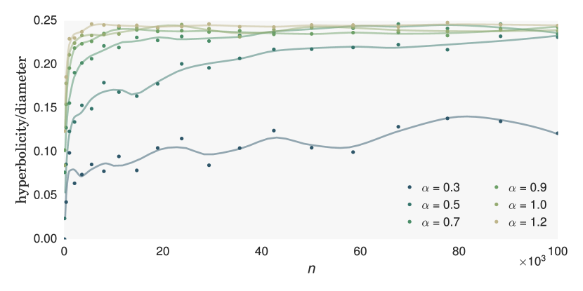
Figure 4: Ratio of hyperbolicity and diameter of $G(n,m,p)$ for different values of $\alpha$ and increasing $n$. The parameters $\beta=\gamma=1.2$ were kept constant and all data points were averaged over 20 graphs. Due to error propagation, the error bars are large and we omit them for the sake of clarity. Lines represent a smoothed version of the series and are included as a visual guide.

Table 2: Estimated asymptotic values of the plots in Figure 4, obtained by averaging the series’ last $11$ values. As seen on the right, the values fit the logistic function $.24(1+2^{-15.21(\alpha-.31)})^{-1}$ well (residuals plotted in lower portion).

$\alpha$	$\hat{d}$
0.3	0.115
0.5	0.213
0.7	0.237
0.9	0.237
1.0	0.240
1.2	0.245

 

The asymptotic bounds provided by Lemma 9 are incredibly pessimistic: For parameters $\alpha=1.5$, $\gamma=5$ and $\beta=0.1$ (selected to be relatively realistic and enable easy generation) the bound on $\widetilde{\nabla}\!_{r}$ provided by this lemma is at least $10^{13}$ (independent of $r$) even if we only insist on an error probability of $O(n^{-1})$. Since all tools for classes of bounded expansion depend heavily on the behavior of the expansion function and the expansion function given by the framework in [31] will depend on $\delta_{r}$, this upper bound is not enough to show practical applicability. Our experiment provides empirical evidence that the upper bound is not tight, improving the prospects for these associated tools. Specifically, we calculate so-called $p$-centered colorings, which can be used to characterize classes of bounded expansion and have immediate algorithmic applications [31].

Proposition 2 ($p$-centered colorings [31])

A graph class $\mathcal{G}$ has bounded expansion if and only if there exists a function $f$ such that for every $G\in\mathcal{G}$, $p\in\mathbf{N}$, the graph $G$ can be colored with $f(p)$ colors so that any $i<p$ color classes induce a graph of treewidth $\leqslant i$ in $G$. This coloring can be computed in linear time.

The characterization can be made stronger (the colorings are actually low treedepth colorings), but this fact is not important in this context. We implemented a simple version of the linear time coloring algorithm and ran it on ten random intersection graphs for each ($n\in\{500$, $1000$, $\dots$, $6000$, $7000$,$\dots$, $10,000$, $15,000$, $20,000$, $25,000\}$) with parameters $\alpha=1.5$, $\gamma=5$ and $\beta=0.1$ for each $p\in\{2,3,4,5\}$. Figure 5 shows the median number of colors used by the algorithm. Our theoretical results predict a horizontal asymptote for every $p$. We can see a surprisingly small bound for $p\in\{2,3,4\}$. Even for $p=5$ the plot starts flattening within the experimental range. It should be noted that the colorings given by this simple approximation algorithm are very likely to be far from optimal (i.e. the colorings may use many unnecessary colors).

This result indicates that the graphs modeled by random intersection are amenable to algorithms based on $p$-centered colorings (which usually perform dynamic programming computations that depend exponentially on the number of colors). Further, by the known relation between $p$-centered colorings and the expansion function, these experiments indicate that these graphs have much more reasonable expansion bounds than Lemma 9 would suggest.

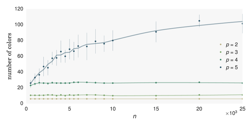
Figure 5: Median number of colors in a $p$-centered coloring for $G(n,m,p)$ with parameters $\alpha=1.5$, $\beta=0.1$ and $\gamma=5$ (taken over ten random instances). Error bars denote one standard deviation (for $p\leqslant 4$ hardly visible). Lines represent a smoothed versions of the series and are included as a visual guide.

6 Conclusion and open problems

In this paper we have determined the conditions under which random intersection graphs exhibit two types of algorithmically useful structure. We proved graphs in $G(n,m,p)$ are structurally sparse (have bounded expansion) precisely when the number of attributes in the associated bipartite graph grows faster than the number of vertices ($\alpha>1$). Moreover, we showed that when the generated graphs are not structurally sparse, they fail to achieve even much weaker notions of sparsity (in fact, w.h.p. they contain large cliques).

On the other hand, we showed that the metric structure of random intersection graphs is not tree-like for any value of $\alpha$: the hyperbolicity (and treelength) grows at least logarithmically in $n$. While we only determine a lower bound for the hyperbolicity, we believe this bound to be the correct order of magnitude since the diameter (a natural upper bound for the hyperbolicity) of a similar model of random intersection graphs was shown to be $O(\log n)$ [40]. Our experimental results support this hypothesis: the ratio of hyperbolicity to diameter seems to converge to a constant.

A question that naturally arises from these results is if structural sparsity should be an expected characteristic of practically relevant random graph models. Our contribution solidifies this idea and supports previous results for different random graph models [13, 39]. We further ask whether the grad is small enough to enable practical algorithmic application—our empirical evaluation using $p$-centered colorings of random intersection graphs with $\alpha>1$ indicate the answer is affirmative.

Acknowledgments: The authors would like to thank Kevin Jasik of RWTH Aachen University for generating the data for the $p$-centered coloring experiment. Portions of this research are a product of work started during the ICERM research cluster “Towards Efficient Algorithms Exploiting Graph Structure”, co-organized by B. Sullivan, E. Demaine, and D. Marx in April 2014. N. Lemons funded by the Department of Energy at Los Alamos National Laboratory under contract DE-AC52-06NA25396 through the Laboratory-Directed Research and Development Program. F. Sánchez Villaamil funded by DFG-Project RO 927/13-1 “Pragmatic Parameterized Algorithms”. B. D. Sullivan supported in part by DARPA GRAPHS/SPAWAR Grant N66001-14-1-4063, the Gordon & Betty Moore Foundation under DDD Investigator Award GBMF4560, and the National Consortium for Data Science. Any opinions, findings, and conclusions or recommendations expressed in this publication are those of the author(s) and do not necessarily reflect the views of DARPA, SSC Pacific, DOE, the Moore Foundation, or the NCDS.

References

- [1] V. Batagelj and M. Zaversnik. An algorithm for cores decomposition of networks. CoRR, cs.DS/0310049, 2003.
- [2] M. Behrisch. Component evolution in random intersection graphs. Electronic Journal of Combinatorics, 14, 2007.
- [3] M. Bloznelis. Degree and clustering coefficient in sparse random intersection graphs. Annals of Applied Probability, 23:1254–1289, 2013.
- [4] M. Bloznelis, J. Jaworski, and V. Kurauskas. Assortativity and clustering of sparse random intersection graphs. Electronic Journal of Probability, 18:1–24, 2013.
- [5] M. Bloznelis and V. Kurauskas. Large cliques in sparse random intersection graphs. ArXiv pre-print arXiv:1302.4627, February 2013.
- [6] M. Borassi, D. Coudert, P. Crescenzi, and A. Marino. On computing the hyperbolicity of real-world graphs. In Algorithms-ESA 2015, pages 215–226. Springer, 2015.
- [7] M. Bridson and A. Häfliger. Metric Spaces of Non-Positive Curvature. Grundlehren Der Mathematischen Wissenschaften. Springer, 2009.
- [8] V. Chepoi, F. F. Dragan, B. Estellon, M. Habib, and Y. Vaxès. Diameters, centers, and approximating trees of -hyperbolic geodesic spaces and graphs. In Symposium on Computational Geometry, pages 59–68, 2008.
- [9] N. Cohen, D. Coudert, and A. Lancin. On computing the Gromov hyperbolicity. Journal of Experimental Algorithmics, 20:1.6:1–1.6:18, August 2015.
- [10] P. Crescenzi, R. Grossi, M. Habib, L. Lanzi, and A. Marino. On computing the diameter of real-world undirected graphs. Theoretical Computer Science, 514:84–95, 2013.
- [11] P. Crescenzi, R. Grossi, C. Imbrenda, L. Lanzi, and A. Marino. Finding the diameter in real-world graphs. In Algorithms–ESA 2010, pages 302–313. Springer, 2010.
- [12] M. Deijfen and W. Kets. Random intersection graphs with tunable distribution and clustering. Probability in the Engineering and Informational Sciences, 23:661–674, 2009.
- [13] E. D. Demaine, F. Reidl, P. Rossmanith, F. Sánchez Villaamil, S. Sikdar, and B. D. Sullivan. Structural sparsity of complex networks: Bounded expansion in random models and real-world graphs. CoRR, abs/1406.2587, 2014.
- [14] The Sage Developers. SageMath, the Sage Mathematics Software System (Version 7.1.0), 2016. http://www.sagemath.org.
- [15] Z. Dvořák, D. Král, and Robin Thomas. Testing first-order properties for subclasses of sparse graphs. Journal of the ACM, 60(5):36, 2013.
- [16] H. Fournier, A. Ismail, and A. Vigneron. Computing the Gromov hyperbolicity of a discrete metric space. Information Processing Letters, 115(6):576–579, June 2015.
- [17] E. Godehardt, J. Jarowski, and K. Rybarczyk. Clustering coefficients of random intersection graphs. In Challenges at the interface of data analysis computer science and optimization, pages 243–253. Springer, 2012.
- [18] M. Gromov. Hyperbolic groups. In Essays in group theory, pages 75–263. Springer, 1987.
- [19] A. A. Hagberg, Daniel A. Schult, and Pieter J. Swart. Exploring network structure, dynamics, and function using NetworkX. In Proceedings of the 7th Python in Science Conference (SciPy2008), pages 11–15, Pasadena, CA USA, August 2008.
- [20] J. Jaworski, M. Karoński, and D. Stark. The degree of a typical vertex in generalized random intersection graph models. Discrete Mathematics, 306:2152–2165, 2006.
- [21] E. Jonckheere, P. Lohsoonthorn, and F. Bonahon. Scaled Gromov hyperbolic graphs. Journal of Graph Theory, 57(2):157–180, 2008.
- [22] E. Jones, T. Oliphant, and P. Peterson. SciPy: open source scientific tools for Python. 2014.
- [23] M. S. E. Karoński and K. Singer-Cohen. On random intersection graphs: the subgraph problem. Combinatorics, Probability and Computing, 8:131–159, 1999.
- [24] R. Kleinberg. Geographic routing using hyperbolic space. In IEEE INFOCOM 2007-26th IEEE International Conference on Computer Communications, pages 1902–1909, 2007.
- [25] A. N. Lagerås and M. Lindholm. A note on the component structure in random intersection graphs with tunable clustering. Electronic Journal of Combinatorics, 15, 2008.
- [26] K. Levenberg. A method for the solution of certain non–linear problems in least squares. 1944.
- [27] C. Magnien, M. Latapy, and M. Habib. Fast computation of empirically tight bounds for the diameter of massive graphs. Journal of Experimental Algorithmics (JEA), 13:10, 2009.
- [28] D.W. Marquardt. An algorithm for least-squares estimation of nonlinear parameters. Journal of the society for Industrial and Applied Mathematics, 11(2):431–441, 1963.
- [29] O. Narayan and I. Saniee. Large-scale curvature of networks. Physical Review E, 84:066108, Dec 2011.
- [30] O. Narayan, I. Saniee, and G.H. Tucci. Lack of spectral gap and hyperbolicity in asymptotic Erdös-Renyi sparse random graphs. In Communications Control and Signal Processing (ISCCSP), 2012 5th International Symposium on, pages 1–4. IEEE, 2012.
- [31] J. Nešetřil and P. Ossona de Mendez. Grad and classes with bounded expansion I. and II. European Journal of Combinatorics, 29(3):760–791, 2008.
- [32] J. Nešetřil and P. Ossona de Mendez. First order properties on nowhere dense structures. The Journal of Symbolic Logic, 75(3):868–887, 2010.
- [33] J. Nešetřil and P. Ossona de Mendez. On nowhere dense graphs. European Journal of Combinatorics, 32(4):600–617, 2011.
- [34] J. Nešetřil and P. Ossona de Mendez. Sparsity: Graphs, Structures, and Algorithms, volume 28 of Algorithms & Combinatorics. Springer, 2012.
- [35] J. Nešetřil, P. Ossona de Mendez, and D. R. Wood. Characterisations and examples of graph classes with bounded expansion. European Journal of Combinatorics, 33(3):350–373, 2012.
- [36] M. E. J. Newman, S. H. Strogatz, and D. J. Watts. Random graphs with arbitrary degree distributions and their applications. Physical Review E, 64(2), 2001.
- [37] M. P. O’Brien et al. CONCUSS: Version 1.0, September 2015. 10.5281/zenodo.30281.
- [38] B. Pittel, J. Spencer, and N. Wormald. Sudden emergence of a giant -core in a random graph. Journal of Combinatorial Theory, Series B, 67(1):111–151, 1996.
- [39] F. Reidl. Structural sparseness and complex networks. Dr., Aachen, Techn. Hochsch., Aachen, 2016. Aachen, Techn. Hochsch., Diss., 2015.
- [40] K. Rybarczyk. Diameter, connectivity, and phase transition of the uniform random intersection graph. Discrete Mathematics, pages 1998–2019, 2011.
- [41] K. Rybarczyk. The coupling method for inhomogeneous random intersection graphs. Preprint. arXiv:1301.0466, 2013.
- [42] Y. Shang. Lack of Gromov-hyperbolicity in small-world networks. Open Mathematics, 10(3):1152–1158, 2012.
- [43] Y. Shang. Non-hyperbolicity of random graphs with given expected degrees. Stochastic Models, 29(4):451–462, 2013.
- [44] K. Singer-Cohen. Random intersection graphs. PhD thesis, Department of Mathematical Sciences, The Johns Hopkins University, 1995.
- [45] F. W. Takes and W. A. Kosters. Computing the eccentricity distribution of large graphs. Algorithms, 6(1):100, 2013.
- [46] D. J. Watts and S. H. Strogatz. Collective dynamics of ‘small-world’ networks. Nature, 393:440–442, 1998.
- [47] W. Wei, W. Fang, G. Hu, and M.W. Mahoney. On the hyperbolicity of small-world and treelike random graphs. Internet Mathematics, 9(4):434–491, 2013.