Multipatch Discontinuous Galerkin Isogeometric Analysis

Abstract

Isogeometric analysis (IgA) uses the same class of basis functions for both, representing the geometry of the computational domain and approximating the solution. In practical applications, geometrical patches are used in order to get flexibility in the geometrical representation. This multi-patch representation corresponds to a decomposition of the computational domain into non-overlapping subdomains also called patches in the geometrical framework. We will present discontinuous Galerkin (dG) methods that allow for discontinuities across the subdomain (patch) boundaries. The required interface conditions are weakly imposed by the dG terms associated with the boundary of the sub-domains. The construction and the corresponding discretization error analysis of such dG multi-patch IgA schemes will be given for heterogeneous diffusion model problems in volumetric 2d and 3d domains as well as on open and closed surfaces. The theoretical results are confirmed by numerous numerical experiments which have been performed in G+Smo. The concept and the main features of the IgA library G+Smo are also described.

1 Indroduction

The Isogeometric analysis (IgA), which was introduced by Hughes, Cottrell and Bazilevs in 2005, is a new discretization technology which uses the same class of basis functions for both, representing the geometry of the computational domain and approximating the solution of problems modeled by Partial Differential Equations (PDEs), LMMT_HughesCottrellBazilevs:2005a . IgA uses the exact geometry in the class of Computer Aided Design (CAD) geometries, and thus geometrical errors introduced by approximation of the physical domain are eliminated. This feature is especially important in technical applications where the CAD geometry description is directly used in the production process. Usually, IgA uses basis functions like B-Splines and Non-Uniform Rational B-Splines (NURBS), which are standard in CAD, and have several advantages which make them suitable for efficient and accurate simulation, see LMMT_CottrellHughesBazilevs:2009a . The mathematical analysis of approximation properties, stability and discretization error estimates of NURBS spaces have been well studied in LMMT_BazilevsBeiraoCottrellHughesSangalli:2006a . Furthermore, approximation error estimates due to mesh, polynomial degree and smoothness refinement have been obtained in LMMT_BeiraoBuffaRivasSangalli:2010a , and likewise a hybrid method that combines a globally $C^{1}-$continuous, piecewise polynomial finite element basis with rational NURBS-mappings have also been considered in LMMT_KleissJuettlerZulehner:2012a .

In practical applications, the computational domain $\Omega\subset\mathbb{R}^{d}$ ($d=2,3$) is usually represented by multiple patches leading to non-matching meshes and thus to patch-wise non-conforming approximation spaces. In order to handle non-matching meshes and polynomial degrees across the patch interfaces, the discontinuous Galerkin (dG) technique that is now well established in the Finite Element Analysis (FEA) of different field problems is employed. Indeed, dG methods have been developed and analyzed for many applications including elliptic, parabolic and hyperbolic PDEs. The standard dG finite element methods use approximations that are discontinuous across the boundaries of every finite element of the triangulation. To achieve consistent, stable and accurate schemes, some conditions are prescribed on the inter-element boundaries, see, e.g., Rivière’s monograph LMMT_Riviere:2008a .

In this paper, we present and analyze multipatch dG IgA methods for solving elliptic PDEs in volumetric 2d or 3d computational domains as well as on open and closed surfaces. As model problems, we first consider diffusion problems of the form

$$-\nabla\cdot(\alpha\nabla u)={f}{\ }\text{in}{\ }\Omega,{\ }\text{and}{\ }{u}={u}_{D}{\ }\text{on $\partial\Omega$},$$ (1)

where $\Omega$ is a bounded Lipschitz domain in $\mathbb{R}^{d},{\ }d=2,3$, with the boundary $\partial\Omega$, $f$ is a given source term, and $u_{D}$ are given Dirichlet data. Neumann, Robin and mixed boundary conditions can easily be treated in the same dG IgA framwork which we are going to analyze in this paper. The same is true for including a reaction term into the PDE (1). The diffusion coefficient $\alpha$ is assumed to be bounded from above and below by strictly positive constants. We allow $\alpha$ to be discontinuous across the inter-patch boundaries with possible large jumps across these interfaces. More precisely, the computational domain $\Omega$ is subdivided into a collection $\mathcal{T}_{H}(\Omega):=\{\Omega_{i}\}_{i=1}^{N}$ of non-overlapping subdomains (patches) $\Omega_{1},\ldots,\Omega_{N}$, where the patches $\Omega_{i}$ are obtained by some NURBS mapping $\Phi_{i}$ from the parameter domain $\widehat{\Omega}=(0,1)^{d}\subset\mathbb{R}^{d}$. In every subdomain, the problem is discretized under the IgA methodology. The dG IgA method is considered in a general case without imposing any matching grid conditions and without any continuity requirements for the discrete solution across the interfaces $F_{ij}=\partial\Omega_{i}\cap\partial\Omega_{j}$. Thus, on the interfaces, the dG technique ensures the communication of the solution between the adjacent subdomains. For simplicity, we assume that the coefficients are piecewise constant with respect to the decomposition $\mathcal{T}_{H}(\Omega_{i})_{i=1}^{N}$. It is well known that solutions of elliptic problems with discontinuous coefficients are generally not smooth LMMT_Kellog:1975a ; LMMT_Grisvard:2011a , Thus, we cannot expect that the dG IgA provides convergence rates like in the smooth case. Here, the reduced regularity of the solution is of primary concern. Following the techniques developed by Di Pietro and Ern LMMT_DiPietroErn:2012a ; LMMT_DiPietroErn:2012b for dG FEA, we present an error analysis for diffusion problems in 2d and 3d computational domains with solutions belonging to $W^{l,p}(\Omega_{i}),\,l\geq 2,{\ }p\in(\max\{1,{2d}/{(d+2(l-1))}\},2],\,i=1,\ldots,N$. In correspondence with this regularity, we show optimal convergence rates of the discretization error in the classical “broken” dG - norm. Due to the peculiarities of the dG IgA, the proofs are quite technical and can be found in the paper LMMT_LangerToulopoulos:2014a written by two of the co-authors. Solutions of elliptic problems with low regularity can also appear in other cases. For example, geometric singular boundary points (re-entrant corners), points with change of the boundary conditions, and singular source terms can cause low-regularity solutions as well, see, e.g., LMMT_Grisvard:2011a . Especially, in the IgA, we want to use the potential of the approximation properties of NURBS based on high-order polynomials. In this connection, the error estimates obtained for the low-regularity case can be very useful. Indeed, via mesh grading, that has been used in the FEA for a long time LMMT_OganesjanRuchovetz:1979a ; LMMT_ApelMilde1996 , we can recover the full convergence rate corresponding to the underlying polynomial degree. We mention that in the literature other techniques have been proposed for solving two dimensional problems with singularities. For example, in LMMT_OhKimJeong:2013a and LMMT_JeongOhKangKim:2013a , the original B-Spline finite dimensional space has been enriched by generating singular functions which resemble the types of the singularities of the problem. Also in LMMT_SangalliaNurbs2012 , by studying the anisotropic character of the singularities of the problem, the one dimensional approximation properties of the B-Splines are generalized in order to produce anisotropic refined meshes in the regions of the singular points. Our error analysis is accompanied by a series of numerical tests which fully confirm our convergence rate estimates for the multipatch dG IgA in both the full and the low regularity cases as well as the recovering of the full rate by means of mesh grading techniques. It is very clear that our analysis can easily be generalized to more general classes of elliptic boundary value problems like plane strain or stress linear elasticity problems or linear elasticity problems in 3d volumetric computational domains.

We will also consider multipatch dG IgA of diffusion problems of the form (1) on sufficiently smooth, open and closed surfaces $\Omega$ in $\mathbb{R}^{3}$, where the gradient $\nabla$ must now be replaced by the surface gradient $\nabla_{\Omega}$, see, e.g., LMMT_DziukElliott:2013a , and the patches $\Omega_{i}$, into which $\Omega$ is decomposed, are now images of the parameter domain $\widehat{\Omega}=(0,1)^{2}$ by the mapping $\Phi_{i}:\widehat{\Omega}\subset\mathbb{R}^{2}\rightarrow\Omega_{i}\subset\mathbb{R}^{3}$. The case of matching meshes was considered and analyzed in LMMT_LangerMoore:2014a by two of the co-authors, see also LMMT_ZhangXuChen2014a for a similar work. It is clear that the results for non-matching spaces and for mesh grading presented here for the volumetric (2d and 3d) case can be generalized to diffusion problems on open and closed surfaces. Until now, the most popular numerical method for solving PDEs on surfaces is the surface Finite Element Method (FEM). The surface FEM was first applied to compute approximate solutions of the Laplace-Beltrami problem, where the finite element solution is constructed from the variational formulation of the surface PDEs in the finite element space that is living on the triangulated surface approximating the real surface LMMT_Dziuk:1988a . This method has been extended to the parabolic equations fixed surfaces by Dziuk and Elliot LMMT_DziukElliott:2007b . To treat conservation laws on moving surfaces, Dziuk and Elliot proposed the evolving surface finite element methods, see LMMT_DziukElliott:2007a . Recently, Dziuk and Elliot have published the survey paper LMMT_DziukElliott:2013a which provides a comprehensive presentation of different finite element approaches to the solution of PDEs on surfaces with several applications. The first dG finite element scheme, which extends Dziuk’s approach, was proposed by Dedner et al. LMMT_DednerMadhavanStinner:2013a and has very recently been extended to adaptive dG surface FEM LMMT_DednerMadhavan:2014a and high-order dG finite element approximations on surfaces LMMT_AntoniettiDednerMadhavanStangalioStinnerVeran:2014a . However, since all these approaches rely on the triangulated surface, they have an inherent geometrical error which becomes more complicated when approximating problems with complicated geometries. This drawback of the surface FEM can be overcome by the IgA technology, at least, in the class of CAD surfaces which can be represented exactly by splines or NURBS. Dede and Quateroni have introduced the surface IgA for fixed surfaces which can be represented by one patch LMMT_DedeQuarteroni:2012a . They presented convincing numerical results for several PDE problems on open and closed surfaces. However, in many practical applications, it is not possible to represent the surface $\Omega$ with one patch. The surface multipatch dG IgA that allows us to use patch-wise different approximations spaces on non-matching meshes is then the natural choice.

The new paradigm of IgA brings challenges regarding the implementation. Even though the computational domain is partitioned into subdomains (patches) and elements (parts of the domain delimited by images of knot-lines or knot-planes), the information that is accessible by the data structure (parametric B-spline patches) is quite different than that of a classical finite element mesh (soup of triangles or simplices). In this realm, existing finite element software libraries cannot easily be adapted to the isogeometric setting. Apart from the data structures used, another issue is the fact that FEA codes are focused on treating nodal shape function spaces, contrary to isogeometric function spaces. To provide a unified solution to the above (and many other) issues, we present the Geometry and Simulation Modules (G+Smo ) library, which provides a unified, object-oriented development framework suitable to implement advanced isogeometric techniques, such as dG methods.

The rest of the paper is organized as follows. In Section 2, we present and analyze the multipatch dG IgA for diffusion problems in volumetric 2d and 3d computational domains including the case of low-regularity solutions. We also study the mesh grading technology which allows us to recover the full convergence rates defined by the degree $k$ of the underlying polynomials. The numerical analysis is accompanied by numerical experiments fully confirming the theoretical results. Section 3 is devoted to multipatch dG IgA of diffusion problems on open and closed surfaces. We present and discuss new numerical results including the case of jumping coefficients and non-matching meshes. The concept and the main features of the G+Smo library is presented in Section 4. All numerical experiments presented in this paper have been preformed in G+Smo.

2 Multipatch dG IgA for PDEs in 3d Computational Domains

2.1 Multipatch dG IgA Discretization

The weak formulation of (1) reads as follows: find a function $u$ from the Sobolev space $W^{1,2}(\Omega)$ such that $u=u_{D}$ on $\partial\Omega$ and satisfies the variational formulation

$$a(u,v)=l(v),{\ }\forall v\in W^{1,2}_{0}(\Omega):=\{v\in W^{1,2}(\Omega):\,v=0\;\mbox{on}\;\partial\Omega\},$$ (2)

where the bilinear form $a(\cdot,\cdot)$ and the linear form $l(\cdot)$ are defined by the relations

$$a(u,v)=\int_{\Omega}\alpha\nabla u\cdot\nabla v\,dx\quad\text{and}\quad l(v)=\int_{\Omega}fv\,dx,$$

respectively. Beside Sobolev’s Hilbert spaces $H^{l}(\Omega)=W^{l,2}(\Omega)$, we later also need Sobolev’s Banach spaces $W^{l,p}(\Omega)$, $p\in[1,\infty)$, see, e.g., LMMT_AdamsFournier:2008 . The existence and uniqueness of the solution $u$ of problem (2) can be derived by Lax-Milgram’s Lemma LMMT_LCEvans:1998a . In order to apply the IgA methodology to problem (1), the domain $\Omega$ is subdivided into a union of subdomains $\mathcal{T}_{H}(\Omega):=\{\Omega_{i}\}_{i=1}^{N}$ such that

$$\bar{\Omega} =\bigcup_{i=1}^{N}\bar{\Omega}_{i},\quad\text{with}\quad\Omega_{i}\cap\Omega_{j}=\emptyset,{\ }\text{if}{\ }j\neq i.$$ (3)

As we mentioned in the introduction, the subdivision of $\Omega$ is assumed to be compatible with the discontinuities of $\alpha$, i.e. they are constant in the interior of $\Omega_{i}$, that is $\alpha|_{\Omega_{i}}:=\alpha^{(i)}$, and their discontinuities appear only across the interfaces $F_{ij}=\partial\Omega_{i}\cap\partial\Omega_{j}$, cf., e.g., LMMT_Dryja:2003a ; LMMT_DiPietroErn:2012a ; LMMT_DiPietroErn:2012b . Throughout the paper, we will use the notation $a\sim b$ meaning that there are positive constants $c$ and $C$ such that $ca\leq b\leq Ca$.

As it is common in IgA, we assume a parametric domain $\widehat{\Omega}$ of unit length, e.g., $\widehat{\Omega}=(0,1)^{d}$. For any $\Omega_{i}$, we associate $d$ knot vectors $\Xi^{(i)}_{n}$, $n=1,...,d$, on $\widehat{\Omega}$, which create a mesh $T^{(i)}_{h_{i},\widehat{\Omega}}=\{\hat{E}_{m}\}_{m=1}^{M_{i}}$, where $\hat{E}_{m}$ are the micro-elements, see details in LMMT_HughesCottrellBazilevs:2005a . We refer to $T^{(i)}_{h_{i},\widehat{\Omega}}$ as the parametric mesh of $\Omega_{i}$. For every $\hat{E}_{m}\in T^{(i)}_{h_{i},\widehat{\Omega}}$, we denote by $h_{\hat{E}_{m}}$ its diameter and by $h_{i}=\max\{h_{\hat{E}_{m}}\}$ the mesh size of $T^{(i)}_{h_{i},\widehat{\Omega}}$. We assume the following properties for every $T^{(i)}_{h_{i},\widehat{\Omega}}$:

• quasi-uniformity: for every $\hat{E}_{m}\in T^{(i)}_{h_{i},\widehat{\Omega}}$ holds ${h}_{i}\sim h_{\hat{E}_{m}}$,

• for the micro-element edges $e_{\hat{E}_{m}}\subset\partial\hat{E}_{m}$ holds $h_{\hat{E}_{m}}\sim e_{\hat{E}_{m}}$.

On every $T^{(i)}_{h_{i},\widehat{\Omega}}$, we construct the finite dimensional space $\hat{\mathbb{B}}^{(i)}_{h_{i}}$ spanned by ${B}$-spline basis functions of degree $k$, see LMMT_HughesCottrellBazilevs:2005a ,

$$\hat{\mathbb{B}}^{(i)}_{h_{i}}=span\{\hat{B}_{j}^{(i)}(\hat{x})\}_{j=0}^{dim(\hat{\mathbb{B}}_{h_{i}}^{(i)})},$$ (4)

where every basis function $$\hat{B}_{j}^{(i)}(\hat{x}) B$$ in (4) is derived by means of tensor products of one-dimensional -spline basis functions, e.g.,

$$\hat{B}_{j}^{(i)}(\hat{x})=\hat{B}_{j_{1}}^{(i)}(\hat{x}_{1})\cdot\cdot\cdot\hat{B}_{j_{d}}^{(i)}(\hat{x}_{d}).$$ (5)

For simplicity, we assume that the basis functions of every $\hat{\mathbb{B}}_{h_{i}}^{(i)},i=1,...,N$, are of the same degree $k$.

Every subdomain $\Omega_{i}\in\mathcal{T}_{H}(\Omega)$, $i=1,...,N$, is exactly represented through a parametrization (one-to-one mapping), cf. LMMT_HughesCottrellBazilevs:2005a , having the form

$$\Phi_{i}:\widehat{\Omega}\rightarrow\Omega_{i}, \quad\Phi_{i}(\hat{x})=\sum_{j}C^{(i)}_{j}\hat{B}_{j}^{(i)}(\hat{x}):=x\in\Omega_{i},$$ (6)

where $C_{j}^{(i)}$ are the control points and $\hat{x}={\Psi}_{i}(x):=\Phi^{-1}_{i}(x)$. Using $\Phi_{i}$, we construct a mesh $T^{(i)}_{h_{i},\Omega_{i}}=\{E_{m}\}_{m=1}^{M_{i}}$ for every $\Omega_{i}$, whose vertices are the images of the vertices of the corresponding mesh $T^{(i)}_{h_{i},\widehat{\Omega}}$ through $\Phi_{i}$. If $h_{\Omega_{i}}=\max\{h_{E_{m}}:{\ }E_{m}\in T^{(i)}_{h_{i},\Omega_{i}}\}$ is the subdomain $\Omega_{i}$ mesh size, then, based on definition (6) of $\Phi_{i}$, we have the equivalence relation $h_{i}\sim h_{\Omega_{i}}.$

The mesh of $\Omega$ is considered to be $T_{h}(\Omega)=\bigcup_{i=1}^{N}T^{(i)}_{h_{i},\Omega_{i}}$, where we note that there are no matching mesh requirements on the interior interfaces $F_{ij}=\partial\Omega_{i}\cap\partial\Omega_{j},i\neq j$. For the sake of brevity in our notations, the interior faces of the boundary of the subdomains are denoted by $\mathcal{F}_{I}$ and the collection of the faces that belong to $\partial\Omega$ by $\mathcal{F}_{B}$, e.g. $F\in\mathcal{F}_{B}$ if there is a $\Omega_{i}$ such that $F=\partial\Omega_{i}\cap\partial\Omega$. We denote the set of all subdomain faces by $\mathcal{F}.$

Lastly, we define the $B$-spline space $\mathbb{B}_{h}(\mathcal{T}_{H}(\Omega))=\mathbb{B}^{(1)}_{h_{1}}\times...\times\mathbb{B}^{(N)}_{h_{N}}$ on $\Omega$, where every $\mathbb{B}^{(i)}_{h_{i}}$ is defined on $T^{(i)}_{h_{i},\Omega_{i}}$ as follows

$$\mathbb{B}^{(i)}_{h_{i}}:=\{B_{h_{i}}^{(i)}|_{\Omega_{i}}:B_{h}^{(i)}(\hat{x})=\hat{B}_{h}^{(i)}\circ\Psi_{i}({x}),{\ }\forall\hat{B}_{h}^{(i)}\in\hat{\mathbb{B}}^{(i)}_{h_{i}}\}.$$ (7)

We assume that the mappings $\Phi_{i}$ are regular in the sense that there exist positive constants $c_{m}$ and $c_{M}$ such that

$$c_{m}\leq|det(J_{i}(\hat{x}))|\leq c_{M},{\ }\text{for}{\ }i=1,...,N,{\ }\text{for all}{\ }\hat{x}\in\hat{\Omega},$$ (8)

where $J_{i}(\hat{x})$ denotes the Jacobian $\partial\Phi_{i}(x)/\partial(\hat{x})$ of the mapping $\Phi_{i}$.

Now, for any $\hat{u}\in W^{m,p}(\hat{\Omega}),m\geq 0,p>1$, we define the function

$$\mathcal{U}(x)=\hat{u}(\Psi_{i}(x)),{\ }x\in\Omega_{i},$$ (9)

and the following relation holds true, see LMMT_LangerToulopoulos:2014a ,

$$C_{m}\|\hat{u}\|_{W^{m,p}(\hat{\Omega}})\leq\|\mathcal{U}\|_{W^{m,p}(\Omega_{i})}\leq C_{M}\|\hat{u}\|_{W^{m,p}(\hat{\Omega})},$$ (10)

where the constants $C_{m}$ and $C_{M}$ depending on $C_{m}:=C_{m}(\max_{m_{0}\leq m}(\|D^{m_{0}}\Phi_{i}\|_{\infty}),$
$\|det(\Psi^{{}^{\prime}}_{i})\|_{\infty})$ and $C_{M}:=C_{M}(\max_{m_{0}\leq m}(\|D^{m_{0}}\Psi_{i}\|_{\infty}),\|det(\Phi^{{}^{\prime}}_{i})\|_{\infty}).$ The usefulness of inequalities (10) in the analysis is the following: every required relation can be proved in the parametric domain and then using (10) we can directly have the expression on the physical subdomain.

We use the $B$-spline spaces $\mathbb{B}^{(i)}_{h}$ defined in (7) for approximating the solution of (2) in every subdomain $\Omega_{i}$. Continuity requirements for $\mathbb{B}_{h}(\mathcal{T}_{H}(\Omega))$ are not imposed on the interfaces $F_{ij}$ of the subdomains, clearly $\mathbb{B}_{h}(\mathcal{T}_{H}(\Omega))\subset L^{2}(\Omega)$ but $\mathbb{B}_{h}(\mathcal{T}_{H}(\Omega))\nsubseteq W^{1,2}(\Omega)$. Thus, problem (2) is discretized by discontinuous Galerkin techniques on $F_{ij}$, see, e.g., LMMT_Dryja:2003a . Using the notation $v_{h}^{(i)}:=v_{h}|_{\Omega_{i}}$, we define the average and the jump of $v_{h}$ on $F_{ij}\in\mathcal{F}_{I}$, respectively, by

$$\{v_{h}\}:=\frac{1}{2}(v_{h}^{(i)}+v_{h}^{(j)}), \quad\text{and}\quad\llbracket v_{h}\rrbracket:=v_{h}^{(i)}-v_{h}^{(j)},$$ (11)

and for $$F_{i}\in\mathcal{F}_{B}$$

$$\{v_{h}\}:=v_{h}^{(i)}, \quad\text{and}\quad\llbracket v_{h}\rrbracket:=v_{h}^{(i)}.$$ (12)

The dG-IgA scheme reads as follows: find $u_{h}\in\mathbb{B}_{h}(\mathcal{T}_{H}(\Omega))$ such that

$$a_{h}(u_{h},v_{h})= l(v_{h})+p_{D}(u_{D},v_{h}),{\ }\forall v_{h}\in\mathbb{B}_{h}(\mathcal{T}_{H}(\Omega)),$$ (13)

where

$$a_{h}(u_{h},v_{h})= \sum_{i=1}^{N}a_{i}(u_{h},v_{h})-\sum_{i=1}^{N}\Big{(}\frac{1}{2}s_{i}(u_{h},v_{h})-p_{i}(u_{h},v_{h})\Big{)},$$ (14)

with the bilinear forms

$$a_{i}(u_{h},v_{h})= \int_{\Omega_{i}}\alpha\nabla u_{h}\nabla v_{h}\,dx,$$

$$s_{i}(u_{h},v_{h})= \sum_{F_{ij}\subset\partial\Omega_{i}}\int_{F_{ij}}\{\alpha\nabla u_{h}\}\cdot\mathbf{n}_{F_{ij}}\llbracket v_{h}\rrbracket+\{\alpha\nabla v_{h}\}\cdot\mathbf{n}_{F_{ij}}\llbracket u_{h}\rrbracket\,ds,$$

$$p_{i}(u_{h},v_{h})= \begin{cases}\sum_{F_{ij}\subset\partial\Omega_{i}}\int_{F_{ij}}\mu\Big{(}\frac{\alpha^{(j)}}{h_{j}}+\frac{\alpha^{(i)}}{h_{i}}\Big{)}\llbracket u_{h}\rrbracket\llbracket v_{h}\rrbracket\,ds,&\text{if}{\ }F_{ij}\in\mathcal{F}_{I}\\ \sum_{F_{i}\subset\partial\Omega_{i}}\int_{F_{i}}\mu\frac{\alpha^{(i)}}{h_{i}}\llbracket u_{h}\rrbracket\llbracket v_{h}\rrbracket\,ds,&\text{if}{\ }F_{i}\in\mathcal{F}_{B}\\ \end{cases}$$

$$p_{D}(u_{D},v_{h})= \sum_{F_{i}\subset\partial\Omega_{i}}\int_{F_{i}}\mu\frac{\alpha^{(i)}}{h_{i}}u_{D}v_{h}\,ds,{\ }{\ }F_{i}\in\mathcal{F}_{B}$$

where $\alpha^{(i)}:=\alpha|_{\Omega_{i}}$ and the unit normal vector $\mathbf{n}_{F_{ij}}$ is oriented from $\Omega_{i}$ towards the interior of $\Omega_{j}$ and the parameter $\mu>0$ will be specified later in the error analysis, cf. LMMT_Dryja:2003a .

For notation convenience in what follows, we will use the following expression

$$\int_{F_{ij}}\mu\big{(}\frac{\alpha^{(j)}}{h_{j}}+\frac{\alpha^{(i)}}{h_{i}}\big{)}\llbracket u_{h}\rrbracket\llbracket v_{h}\rrbracket\,ds,$$

for both cases, $F_{ij}\in\mathcal{F}_{I}$ and $F_{i}\in\mathcal{F}_{B}$. In the latter case, we will assume that $\alpha^{(j)}=0$.

2.2 Auxiliary Results

We will use the following auxiliary results which have been shown in LMMT_LangerToulopoulos:2014a .

Lemma 1

Let $u\in W^{l,p}(\mathcal{T}_{H}(\Omega))$ with $l\geq 2$ and $p>1$. Then there is a positive constant $C$, which is determined according to the $C_{m}$ and $C_{M}$ of (10), such that

$$\int_{{F_{ij}}\subset\partial\Omega_{i}}|u|^{p}\,ds\leq C\Big{(}h_{i}^{-1}\int_{\Omega_{i}}|u|^{p}\,dx+h_{i}^{p-1}\int_{\Omega_{i}}|\nabla u|^{p}\,dx\Big{)}.$$ (15)

Lemma 2

For all $v_{h}\in{\mathbb{B}}^{(i)}_{h_{i}}$ defined on $T^{(i)}_{h_{i},{\Omega_{i}}}$, there is a positive constant $C$, depending on the mesh quasi-uniformity parameters and $C_{m}$ and $C_{M}$ of (10) but not on $h_{i}$, such that

$$\|\nabla v_{h}\|^{p}_{L^{p}({\Omega_{i}})}\leq Ch_{i}^{-p}\|v_{h}\|^{p}_{L^{p}({\Omega_{i}})}.$$ (16)

Lemma 3

For all $v_{h}\in{\mathbb{B}}^{(i)}_{h_{i}}$ defined on $T^{(i)}_{h_{i},{\Omega_{i}}}$ and for all ${F}_{ij}\subset\partial{\Omega_{i}}$, there is a positive constant $C$, which depends on the mesh quasi-uniformity parameters $C_{m}$ and $C_{M}$ of (10) but not on $h_{i}$, such that

$$\|v_{h}\|^{p}_{L^{p}({F_{ij}})}\leq Ch_{i}^{-1}\|v_{h}\|^{p}_{L^{p}({\Omega_{i}})}.$$ (17)

Lemma 4

Let $v_{h}\in{\mathbb{B}}^{(i)}_{h_{i}}$ such that $v_{h}\in W^{l,p}({E})\cap W^{m,q}({E}),{\ }{E}\in T^{(i)}_{h_{i},{\Omega_{i}}}$, and $0\leq m\leq l,{\ }1\leq p,q\leq\infty$. Then there is a positive constant $C$, depended on the mesh quasi-uniformity parameters $C_{m}$ and $C_{M}$ of (10) but not on $h_{i}$, such that

$$|v_{h}|_{W^{l,p}({E})}\leq Ch^{m-l-\frac{d}{q}+\frac{d}{p}}_{i}|v_{h}|_{W^{m,q}({E})}.$$ (18)

2.3 Analysis of the dG IgA Discretization

Next, we study the convergence estimates of the method (13) under the following regularity assumption for the weak solution $u\in W^{1,2}(\Omega)\cap W^{l,p}(\mathcal{T}_{H}(\Omega))$ with $l\geq 2$ and $p\in(\max\{1,\frac{2d}{d+2(l-1)}\},2]$. For simplicity of the presentation, we assume that $l\leq k+1$. Nevertheless, for the case of highly smooth solutions, the estimates given below, see Lemma 5, can be expressed in terms of the underlying polynomial degree $k$. More precisely, the estimate $\delta(l,p,d)=l+(d/2-d/p-1)$, must be replaced by $\delta(l,p,d)=\min\{l+(d/2-d/p-1,k\}$. We use the enlarged space $W_{h}^{l,p}:=W^{1,2}(\Omega)\cap W^{l,p}(\mathcal{T}_{H}(\Omega))+\mathbb{B}_{h}(\mathcal{T}_{H}(\Omega))$, and will show that the dG IgA method converges in optimal rate with respect to $\|.\|_{dG}$ norm

$$\|u\|^{2}_{dG}=\sum_{i=1}^{N}\Big{(}\alpha^{(i)}\|\nabla u^{(i)}\|^{2}_{L^{2}(\Omega_{i})}+p_{i}(u^{(i)},u^{(i)})\Big{)},{\ }u\in W_{h}^{l,2}.$$ (19)

For the error analysis, it is necessary to show the continuity and coercivity properties of the bilinear form $a_{h}(.,.)$ of (14) and interpolation estimates in $\|.\|_{dG}$ norm. We start by providing estimates on how well the quasi-interpolant $\Pi_{h}u$ approximates $u\in W^{l,p}(\Omega_{i})$, see proof in LMMT_LangerToulopoulos:2014a .

Lemma 5

Let $u\in W^{l,p}(\Omega_{i})$ with $l\geq 2$ and $p\in(\max\{1,\frac{2d}{d+2(l-1)}\},2]$ and let $E={\Phi}_{i}({E}),{E}\in T^{(i)}_{h_{i},{\Omega}}$. Then for $0\leq m\leq l\leq k+1$, there exist constants $C_{i}:=C_{i}\big{(}\max_{l_{0}\leq l}(\|D^{l_{0}}{\Phi}_{i}\|_{L^{\infty}(\Omega_{i})}),\|u\|_{W^{l,p}(\Omega_{i})}\big{)}$, such that

$$\sum_{E\in T^{(i)}_{h_{i},\Omega_{i}}}|u-\Pi_{h}u|^{p}_{W^{m,p}(E)}\leq C_{i}h_{i}^{p(l-m)}.$$ (20)

Moreover, we have the following estimates for $F_{ij}=\partial\Omega_{i}\cap\partial\Omega_{j}$:

$$(i) {\ }h_{i}^{\beta}\|\nabla u^{(i)}-\nabla\Pi_{h}u^{(i)}\|^{p}_{L^{p}(F_{ij})}\leq C_{i}C_{d,p}h_{i}^{p(l-1)-1+\beta},$$

$$(ii) {\ }\big{(}\frac{\alpha^{(j)}}{h_{j}}+\frac{\alpha^{(i)}}{h_{i}}\big{)}\|\llbracket u-\Pi_{h}u\rrbracket\|^{2}_{L^{2}(F_{ij})}\leq$$

$$\quad C_{i}\alpha^{(j)}\frac{h_{i}}{h_{j}}\Big{(}h_{i}^{\delta(l,p,d)}\|u\|^{p}_{W^{l,p}(\Omega_{i})}\Big{)}^{2}+C_{j}\alpha^{(i)}\frac{h_{j}}{h_{i}}\Big{(}h_{j}^{\delta(l,p,d)}\|u\|_{W^{l,p}(\Omega_{j})}\Big{)}^{2}+$$

$$\qquad C_{j}\Big{(}h_{j}^{\delta(l,p,d)}\|u\|_{W^{l,p}(\Omega_{j})}\Big{)}^{2}+C_{i}\Big{(}h_{i}^{\delta(l,p,d)}\|u\|_{W^{l,p}(\Omega_{i})}\Big{)}^{2},$$

$$(iii) {\ }\|u-\Pi_{h}u\|^{2}_{dG}\leq\sum_{i=1}^{N}C_{i}\Big{(}h_{i}^{\delta(l,p,d)}\|u\|_{W^{l,p}(\Omega_{i})}\Big{)}^{2}+$$

$$\qquad\qquad\sum_{i=1}^{N}\sum_{F_{ij}\subset\partial\Omega_{i}}C_{i}\alpha^{(j)}\frac{h_{i}}{h_{j}}\Big{(}h_{i}^{\delta(l,p,d)}\|u\|_{W^{l,p}(\Omega_{i})}\Big{)}^{2},$$

where $\delta(l,p,d)=l+(d/2-d/p-1)$.

We mention that the proof of estimate $(iii)$ in Lemma 5 can be derived by using the estimates $(i)$, $(ii)$ and Lemma 1.

Lemma 6

Suppose $u_{h}\in\mathbb{B}_{h}(\mathcal{S}(\Omega))$. There exist a positive constant $C$, independent of $\alpha$ and $h_{i}$, such that

$$a_{h}(u_{h},u_{h})\geq C\,\|u_{h}\|_{dG}^{2},{\ }\;\forall\,u_{h}\in\mathbb{B}_{h}(\mathcal{S}(\Omega)).$$ (21)

Proof

By (13), we have that

$$a_{h}(u_{h},u_{h})=\sum_{i=1}^{N}a_{i}(u_{h},u_{h})-\frac{1}{2}\sum_{i=1}^{N}s_{i}(u_{h},u_{h})+p_{i}(u_{h},u_{h})=$$

$$\sum_{i=1}^{N}\alpha_{i}\|\nabla u_{h}\|^{2}_{L^{2}(\Omega_{i})}-2\sum_{F_{ij}\in\mathcal{F}}\int_{F_{ij}}\{\alpha\nabla u_{h}\}\cdot\mathbf{n}_{F_{ij}}\llbracket u_{h}\rrbracket\,ds$$

$$+\sum_{F_{ij}\in\mathcal{F}}\mu\Big{(}\frac{\alpha^{(i)}}{h_{i}}+\frac{\alpha^{(j)}}{h_{j}}\Big{)}\|\llbracket u_{h}\rrbracket\|^{2}_{L^{2}(F_{ij})}.$$ (22)

For the second term on the right hand side, Lemma 2 and the trace inequality (17) expressed on $F_{ij}\in\mathcal{F}$ yield the bound

$$-\sum_{F_{ij}\in\mathcal{F}}\int_{F_{ij}}\{\alpha\nabla u_{h}\}\cdot\mathbf{n}_{F_{ij}}\llbracket u_{h}\rrbracket\,ds\geq\\ {-C_{1,\varepsilon}\sum_{i=1}^{N}\alpha_{i}\|\nabla u_{h}\|^{2}_{L^{2}(\Omega_{i})}-\sum_{F_{ij}\in\mathcal{F}}\frac{1}{C_{2,\varepsilon}}\Big{(}\frac{\alpha^{(i)}}{h_{i}}+\frac{\alpha^{(j)}}{h_{j}}\Big{)}\|\llbracket u_{h}\rrbracket\|^{2}_{L^{2}(F_{ij})}.}$$ (23)

Inserting (23) into (2.3) and choosing $C_{1,\varepsilon}<1/2$ and $\mu>2/C_{2,\varepsilon}$, we obtain (21). $\Square$

Due to assumed regularity of the solution, the normal interface fluxes $(\alpha\nabla u)|_{\Omega_{i}}\cdot\mathbf{n}_{F_{ij}}$ belongs (in general) to $L^{p}(F_{ij})$. The following bound for the interface fluxes in $\|.\|_{L^{p}}$ setting has been shown in LMMT_LangerToulopoulos:2014a .

Lemma 7

There is a constant $C$ such that the following inequality for $(u,v_{h})\in W_{h}^{l,p}\times\mathbb{B}_{h}(\mathcal{S}(\Omega))$ holds true

$$\sum_{i=1}^{N}\sum_{F_{ij}\subset\partial\Omega_{i}}\int_{F_{ij}}\{\alpha\nabla u\}\cdot\mathbf{n}_{F_{ij}}\llbracket v_{h}\rrbracket\,ds\leq$$ (24)

$$C\Big{(}\sum_{F_{ij}\in\mathcal{F}}\alpha^{(i)}h_{i}^{1+\gamma_{p,d}}\|\nabla u^{(i)}\|^{p}_{L^{p}(F_{ij})}+ \alpha^{(j)}h_{j}^{1+\gamma_{p,d}}\|\nabla u^{(j)}\|^{p}_{L^{p}(F_{ij})}\Big{)}^{\frac{1}{p}}\|v_{h}\|_{dG},$$

$$\text{where}{\ }\gamma_{p,d}=d(p-2)/2.\hskip 56.9055pt\qquad$$

Proof

We use Hölder’s inequality and then the results of Lemmas 3 and 4. $\Square$

Applying similar procedure as this in Lemma 7, we can show for the symmetrizing terms that there is a positive constant independent of grid size such that

$$\sum_{i=1}^{N}\sum_{F_{ij}\subset\partial\Omega_{i}}\int_{F_{ij}}\{\alpha\nabla v_{h}\}\cdot\mathbf{n}_{F_{ij}}\llbracket u\rrbracket\,ds\leq C_{1}\|v_{h}\|_{dG}\|u\|_{dG}.$$ (25)

Using the results (24) and (25), we can show the boundedness of the bilinear form, see details in LMMT_LangerToulopoulos:2014a .

Lemma 8

There is a $C$ independent of $h_{i}$ such that for $(u,v_{h})\in W^{l,p}_{h}\times\mathbb{B}_{h}(\mathcal{S}(\Omega))$

$$a_{h}(u,v_{h})\leq C(\|u\|_{dG}^{p}+\sum_{F_{ij}\in\mathcal{F}}h_{i}^{1+\gamma_{p,d}}\alpha^{(i)}\|\nabla u^{(i)}\|^{p}_{L^{p}(F_{ij})}+$$ (26)

$$h_{j}^{1+\gamma_{p,d}}\alpha^{(j)}\|\nabla u^{(j)}\|^{p}_{L^{p}(F_{ij})}\Big{)}^{\frac{1}{p}}\|v_{h}\|_{dG}.$$

Next, we give the main error estimate for the dG IgA method.

Theorem 2.1

Let $u\in W^{1,2}(\Omega)\cap W^{l,p}(\mathcal{T}_{H}(\Omega))$ be the solution of (2), with $l\geq 2$ and $p\in(\max\{1,\frac{2d}{d+2(l-1)}\},2]$. Let $u_{h}\in\mathbb{B}_{h}(\mathcal{S}(\Omega))$ be the dG IgA solution of (13). Then there are $C_{i}:=C_{i}\Big{(}\max_{l_{0}\leq l}\Big{(}\|D^{l_{0}}{\Phi}_{i}\|_{L^{\infty}(E)}\Big{)},\|u\|_{W^{l,p}(\Omega_{i})}\Big{)}$, such that

$$\|u-u_{h}\|_{dG}\leq \sum_{i=1}^{N}\Big{(}C_{i}\Big{(}h_{i}^{\delta(l,p,d)}+\sum_{F_{ij}\subset\partial\Omega_{i}}\alpha^{(j)}\frac{h_{i}}{h_{j}}h_{i}^{\delta(l,p,d)}\Big{)}\|u\|_{W^{l,p}(\Omega_{i})}\Big{)},$$ (27)

where $\delta(l,p,d)=l+(d/2-d/p-1)$.

Proof

First we need to prove the consistency of $u$, i.e. $u$ satisfies (13). Then, we use a variation of Cea’s Lemma (expressed in the dG framework), the results of Lemmata 6 and 8, as well the quasi-interpolation estimates of Lemma 5. A complete proof can be found in LMMT_LangerToulopoulos:2014a . $\Square$

2.4 Numerical Examples

In this section, we present a series of numerical examples to validate the theoretical results, which have been presented.

Smooth and Low-regularity Solutions

We restrict ourselves to a model problem in $\Omega=(-1,1)^{3}$, with $\Gamma_{D}=\partial\Omega$. The domain $\Omega$ is subdivided into four equal subdomains $\Omega_{i}$, $i=1,...,4$, where for simplicity every $\Omega_{i}$ is initially partitioned into a mesh $T^{(i)}_{h_{i},\Omega_{i}}$, with $h:=h_{i}=h_{j},i\neq j$, and $i,j=1,...,4$. Successive uniform refinements are performed on every $T^{(i)}_{h_{i},\Omega_{i}}$ in order to compute numerically the convergence rates. We set the diffusion coefficient equal to one.

In the first test, the data $u_{D}$ and $f$ in (1) are determined such that the exact solution is $u(x)=\sin(2.5\pi x)\sin(2.5\pi y)\sin(2.5\pi z)$ (smooth test case). The first two columns of Table 1 display the convergence rates. As it was expected, the convergence rates are optimal. In the second case, the exact solution is $u(x)=|x|^{\lambda}$. The parameter $\lambda$ is chosen such that $u\in W^{l,p=1.4}(\Omega)$. Specifically, for $l=2$, we set $\lambda=0.58$ and for $l=3$, we set $\lambda=1.58$. In the last columns of Table 1, we display the convergence rates for degree $k=2$ and $k=3$ in case of having $l=2$ and $l=3$. We observe that, for each of the two different tests, the error in the dG-norm behaves according to the main error estimate given by (27).

Table 1: The numerical convergence rates of the dG IgA method.

	highly smooth		$k=2$		$k=3$
$\frac{h}{2^{s}}$	$k=2$	$k=3$	$l=2$	$l=3$	$l=2$	$l=3$
Convergence rates
$s=0$	-	-	-	-	-	-
$s=1$	0.15	2.91	0.62	0.76	0.24	1.64
$s=2$	2.34	2.42	0.29	1.10	0.28	0.89
$s=3$	2.08	3.14	0.35	1.32	0.47	1.25
$s=4$	2.02	3.04	0.35	1.36	0.36	1.37

Non-Matching Meshes

We consider the boundary value problem (1) with exact solution $u(x,y)=\sin(\pi x)$
$\sin(\pi y)$. The computational domain consist of two unit square patches, $\Omega_{1}=(-1,0)\times(0,1)$ and $\Omega_{2}=(0,1)\times(0,1)$, see Fig. 1 (left). The knot vectors representing the geometry are given by $\Xi_{1}^{(1,2)}=\Xi_{2}^{(1,2)}=\{0,0,1,1\}$. We refine the mesh of the patches to a ratio $R$, i.e., the ratio of the grid sizes is $R={h_{1}}/{h_{2}}$, see Fig. 1 (left). We solved the problem using equal B-spline degree $k$ on all patches. We plot in Fig. 1 (right) the dG IgA solution $u_{h}$ computed with $k=2$. In Fig. 2, we present the decay of the $L_{2}$ and $dG$ errors for $k=1,2,3$ and ratios $R$ from 1 up to 5. In Table 2, we display the convergence rates for large ratio $R=40$. In both cases, we observe that the rates are the expected one and are not affected by the different grid sizes of the meshes.

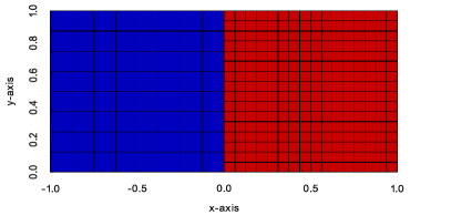
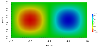
Figure 1: Non-matching meshes: Decomposition into 2 patches with underlying grid of ratio $R=2$ (left), contours of $u_{h}$ (right).

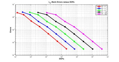
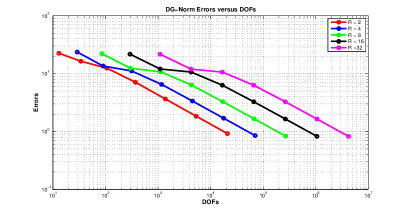
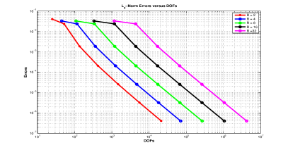
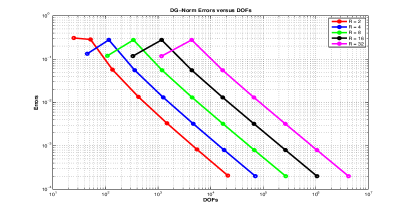
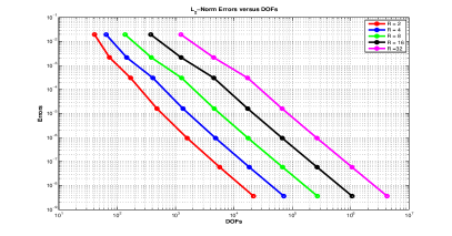
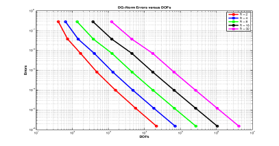
Figure 2: Error decay in the $L_{2}$ (left) and dG (right) norms for polynomial degree $k=1,2,3$ (top to bottom) and ratio $R=2^{r}$ with $r$ running from 1 to 5.

Table 2: Non-Matching Meshes: error estimates for degrees $k=1,2,3$ and $R=40.$

Dofs	$L_{2}$ error	conv. rate	DG error	conv. rate
Degree $k=1$
1685	0.31667	0	2.1596	0
6570	0.0867936	1.86732	0.97857	1.14202
25946	0.0249492	1.79859	0.49992	0.968979
103122	0.00638919	1.96529	0.251392	0.991758
411170	0.00160452	1.99349	0.125887	0.997804
1.64205$\times 10^{6}$	0.000401493	1.9987	0.0629683	0.999435
6.56295$\times 10^{6}$	0.000100393	1.99972	0.0314873	0.999857
Degree $k=2$
1773	0.0330803	0	0.117511	0
6740	0.0237587	0.477516	0.278058	-1.2426
26280	0.00186298	3.67278	0.0555191	2.32433
103784	0.000205886	3.17769	0.0130802	2.0856
412488	2.53126$\times 10^{-5}$	3.02392	0.00321704	2.02358
1.64468$\times 10^{6}$	3.17795$\times 10^{-6}$	2.99369	0.000800278	2.00716
6.5682$\times 10^{6}$	3.99389$\times 10^{-7}$	2.99223	0.000199727	2.00247
Degree $k=3$
1865	0.0196108	0	0.281761	0
6914	0.00216825	3.17704	0.037403	2.91324
26618	0.00030589	2.82545	0.00706104	2.4052
104450	1.60210$\times 10^{-5}$	4.25498	0.000803958	3.13469
413810	9.49748$\times 10^{-7}$	4.07627	9.7687$\times 10^{-5}$	3.04088
1.64731$\times 10^{6}$	5.85542$\times 10^{-8}$	4.0197	1.21191$\times 10^{-5}$	3.01089
6.57346$\times 10^{6}$	3.64710$\times 10^{-9}$	4.00495	1.51195$\times 10^{-6}$	3.00280

2.5 Graded Mesh Partitions for the dG IgA Methods

We saw in the previous numerical tests that the presence of singular points reduce the convergence rates. In this section, we will study this subject in a more general form. We will focus on solving the model problem in domains with re-entrant corners on the boundary. Due to these singular corner points, the regularity of the solution (at least in a small vicinity) is reduced in comparison with the solutions in smooth domains LMMT_Grisvard:1985a ; LMMT_Grisvard:2011a . As a result, the numerical methods applied on quasi uniform meshes for solving these problems do not yield the optimal convergence rate and thus a particular treatment must be applied. We will devise the popularly known graded mesh techniques which have widely been applied so far for finite element methods LMMT_ApelSandingWhiteman:1996 ; LMMT_ApelMilde1996 .

Regularity properties of the solution around the boundary singular points

Let us assume a domain $\Omega\subset\mathbb{R}^{2}$ and let $P_{s}\in\partial\Omega$ be a boundary point with internal angle $\omega\in(\pi,2\pi)$. We consider the local cylindrical coordinates $(r,\theta)$ with pole $P_{s}$, and define the cone, see Fig. 3 (left),

$${\mathcal{C}=\{(x,y)\in\Omega:x=r\cos(\theta),y=r\sin(\theta),0<r<R,0<\theta<\omega\}.}$$ (28)

Then the solution in $\mathcal{C}$ can be written, LMMT_Grisvard:1985a ,

$$u=u_{r}+u_{s},$$ (29)

where $u_{r}\in W^{l\geq 2,2}(\Omega)$ and

$$u_{s}=\xi(r)\gamma r^{\lambda}\sin(\lambda\theta),$$ (30)

where $\gamma$ is the stress intensity factor (is a real number depending only on $f$), and $\lambda={\pi}/{\omega}\in(0,1)$ is an exponent which determines the strength of the singularity. Since $\lambda<1$, by an easy computation, we can show that the singular function $u_{s}$ does not belong to $W^{2,2}(\Omega)$ but $u\in W^{2,p}(\Omega)$ with $p={2}/{2-\lambda}$. The representation (30) of $u_{s}$ helps us to reduce our study to the examination of the behavior of $u$ in the vicinity of the singular point, since the regularity properties of $u$ are determined by the regularity of $u_{s}$. The main idea is the following: based on the a priori knowledge of the analytical form of $u_{s}$ in $\mathcal{C}$, we carefully construct a locally adapted mesh in $\mathcal{C}$ by introducing a grading control parameter $\mu:=\mu(\lambda,k)$, such as allows us to prove that the approximation order of the method applied on this adapted mesh for $u_{s}$ is similar with the order of the method applied on the rest of the mesh (maybe quasi uniform) for $u_{r}$.

The graded mesh for $\mathcal{T}_{H}(\Omega)$ and global approximation estimates

The area $U_{s}:=\{x\in\Omega:|P_{s}-x|\leq R,R\geq N_{Z}h,{\ }N_{Z}\geq 2\}$ is further sub-divided into ring zones $Z_{\zeta},{\ }\zeta=0,..,\zeta_{M}<N_{Z}$, with distance from $P_{s}$ equal to $D_{(Z_{\zeta},P_{s})}:=C(n_{\zeta}h)^{\frac{1}{\mu}}$, where $1\leq n_{\zeta}<N_{Z}$ and $\frac{1}{2}\leq C\leq 1$. The radius of every zone is defined to be $R_{Z_{\zeta}}:=D_{(Z_{\zeta+1},P_{s})}-D_{(Z_{\zeta},P_{s})}=C(n_{\zeta+1}h)^{\frac{1}{\mu}}-C(n_{\zeta}h)^{\frac{1}{\mu}}$.

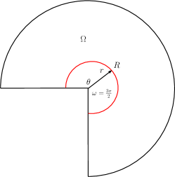
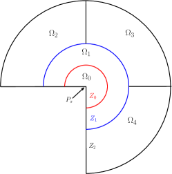
Figure 3: Left: 2d domain with corner singularity. Right: Zone partition and the subdomians $\Omega_{i}$ of $\mathcal{T}_{H}(\Omega)$.

For convenience, we assume that the initial subdivision $\mathcal{T}_{H}$ fulfill the following conditions, for an illustration see Fig. 3 (right) with $\zeta_{M}=2$:

• The subdomains can be grouped into those which belong (entirely) to the area $U_{s}$ and those that belong (entirely) to $\Omega\setminus U_{s}$. This means that there is no $\Omega_{i},{\ }i=1,...,N$ such that $U_{s}\cap\Omega_{i}\neq\emptyset$ and $(\Omega\setminus U_{s})\cap\Omega_{i}\neq\emptyset$.

• Every ring zone $Z_{\zeta}$ is partitioned into “circular” subdomains $\Omega_{i_{\zeta}}$ which have radius $\Omega_{i_{\zeta}}$ equal to the radius of the zone, that is $R_{\Omega_{i_{\zeta}}}=R_{Z_{\zeta}}$. For computational efficiency reasons, we prefer -if its possible- every zone to be only represented by one subdomain.

• The zone $Z_{0}$ is represented by one subdomain, say $\Omega_{0}$, and the mesh $T^{(0)}_{h_{0}}(\Omega_{0})$ includes all $E\in T_{h}(\Omega)$ such that $\partial E\cap P_{s}\neq\emptyset$.

The graded meshes $T^{(i_{\zeta})}_{h_{i_{\zeta}}}(\Omega_{i_{\zeta}})$ are mainly determined by the grading parameter $\mu(\lambda,k)\in(0,1]$ and the mesh sizes $h_{i_{\zeta}}$ are chosen to satisfy the following properties: for $\Omega_{i_{\zeta}}$ with distance $R_{\Omega_{i_{\zeta}}}$ from $P_{s}$, the mesh size $h_{i_{\zeta}}$ is defined to be $h_{i_{\zeta}}=\mathcal{O}(hR_{\Omega_{i_{\zeta}}}^{1-\mu})$ and for $T^{(i_{0})}_{h_{0}}(\Omega_{0})$ the mesh size is of order $h_{i_{0}}=\mathcal{O}(h^{\frac{1}{\mu}})$, more details are given in LMMT_LangerMantzaflarisMooreToulopoulos:2014 . Based on previous properties of the $T^{(i_{\zeta})}_{h_{i_{\zeta}}}(\Omega_{i_{\zeta}})$ meshes, we can conclude the relations

$$C_{m}h^{\frac{1}{\mu}} \leq h_{{i_{\zeta}}}\leq C_{M}h^{\frac{1}{\mu}}, \text{if}{\ }\overline{\Omega}_{i_{\zeta}}\cap P_{s}\neq\emptyset,$$ (31)

$$C_{m}hR_{\Omega_{i_{\zeta}}}^{1-\mu} \leq h_{i_{\zeta}}\leq C_{M}hD_{(Z_{\zeta},P_{s})}^{1-\mu}, \text{if}{\ }\overline{\Omega}_{i_{\zeta}}\cap P_{s}=\emptyset.$$ (32)

Using the local interpolation estimate of Lemma 5 in every $\Omega_{i_{\zeta}}\subset U_{s}$ and the characteristics of the meshes $T^{(i_{\zeta})}_{h_{i_{\zeta}}}(\Omega_{i_{\zeta}})$, we can easily obtain the estimate

$$\|u_{s}-\Pi_{h}u_{s}\|_{dG(U_{s})}\leq\sum_{i_{\zeta}}C_{i_{\zeta}}h_{i_{\zeta}}^{\lambda},$$ (33)

since $u_{s}\in W^{l=1+\lambda,2}(\Omega)$ (and also $u\in W^{2,p=\frac{2}{2-\lambda}}(\Omega)$) and we do not consider nonä-matching grid interfaces. Using the mesh properties (31) and (32), estimate (33) and Lemma 5, we can prove the following global error estimate of the proposed dG IgA method applied to problems with boundary singularities, see LMMT_LangerMantzaflarisMooreToulopoulos:2014 .

Theorem 2.2

Let $Z_{\zeta}$ be a partition of $\Omega\subset\mathbb{R}^{2}$ into ring zones and let $\mathcal{T}_{H}$ to be a sub-division to $\Omega$ with the properties as listed in the previous paragraphs. Let $T_{h_{i}}^{(i)}(\Omega_{i})$ be the meshes of subdomains as described above. Then for the solution $u$ of (2) and the dG IgA solution $u_{h}$, we have the approximation result

$$\|u-u_{h}\|_{dG}\leq Ch^{r},{\ }\text{with}{\ }r=\min(k,{\lambda/\mu}),$$ (34)

where the constant $C>0$ depends on the characteristics of the mesh and on the mappings $\Phi_{i}$ (see (6)) but not on $h_{i}$.

Numerical examples

In this section, we present a series of numerical examples in order to validate the theoretical analysis on the graded mesh in Section 2.5. The first example concerns a two-dimensional problem with a boundary point singularity (L-shape domain). The second example is the interior point singularity problem of the Section 2.4.

1. Boundary Singular Point
   One of the classical test cases is the singularity due to a re-entrant corner. The L-shape domain given by $(-1,1)^{2}\setminus(-1,0)^{2}$. In Fig. 4 (left), the subdivision of $\Omega$ into two subdomains is presented. The exact solution is $u=r^{\frac{\pi}{\omega}}\sin(\theta\pi/\omega),$ where $\omega=3\pi/2$. We set $\Gamma_{D}=\partial\Omega$ and the data ${f},{u}_{D}$ of (2) are specified by the given exact solution. The problem has been solved using $B$-splines of degree $k=1$ and $k=2$ and the grading parameter is $\mu=0.6$ and $\mu=0.3$ respectively. In Fig. 4 (middle), the graded mesh for $\mu=0.6$ is presented and in Fig. 4 (right) the contours of the numerical solution are plotted. In Table 3, we present the convergence rates of the method without grading (left columns). As we can see, the convergence rates are determined by the regularity of the solution around the singular boundary point. In the right columns, we present the convergence rates corresponding to the graded meshes. We can see that the rates tend to be optimal with respect the $B$-spline degree.

   

   

   

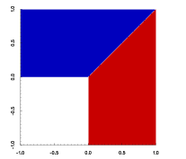
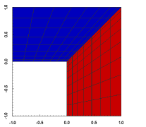
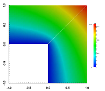
   Figure 4: L-shape test. Left: subdomains, middle: graded mesh with $\mu=0.6$, right: contours of $u_{h}$.

2. Interior Point Singularity
   The domain is $\Omega=(-1,1)^{2}$. We consider a solution ${u}$ of (1) with a point singularity at the origin given by $u(x)=|x|^{\lambda}$. We set $\lambda=0.6$ and is easy to show that $u\in W^{l=1.6,2}(\Omega)$. We set $\alpha=1$ in $\Omega$. In the left columns of Table 3, we display the convergence rates for degrees $k=1$ and $k=2$ without mesh grading. The convergence rates are suboptimal and follow the approximation estimate (27). The problem has been solved again on graded meshes with $\mu=0.6$ for $k=1$ and $\mu=0.3$ for $k=2$, see Fig. 5. We display the convergence rates in the right columns of Table 3. The rates tend to be optimal as it was expected.

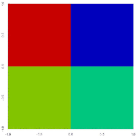
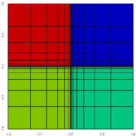
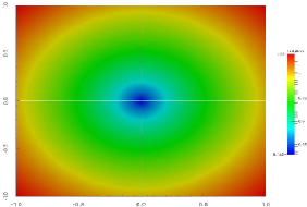
Figure 5: Interior singularity test. Left: the subdomains $\Omega_{i},{\ }i=1,...,4$, middle: the graded mesh with $\mu=0.3$, right: the contours of $u_{h}$.

Table 3: The convergence rates for the L-shape test (left) and for the interior singularity test (right).

	no grading		with grading
$\frac{h}{2^{s}}$	$k=1$	$k=2$	$\begin{matrix}k=1,\\ \mu=0.6\end{matrix}$	$\begin{matrix}k=2,{\ }\\ \mu=0.3\end{matrix}{\ }$
Convergence rates
$s=0$	-	-	-	-
$s=1$	0.636	0.650	0.915	1.672
$s=2$	0.641	0.657	0.933	1.919
$s=3$	0.647	0.661	0.946	1.987
$s=4$	0.652	0.666	0.957	2.071

	no grading		with grading
$\frac{h}{2^{s}}$	$k=1$	$k=2$	$\begin{matrix}k=1,\\ \mu=0.6\end{matrix}$	$\begin{matrix}k=2,{\ }\\ \mu=0.3\end{matrix}{\ }$
Convergence rates
$s=0$	-	-	-	-
$s=1$	0.508	0.573	0.855	1.661
$s=2$	0.547	0.580	0.930	1.828
$s=3$	0.570	0.586	0.969	1.928
$s=4$	0.583	0.591	0.990	1.951

3 Multipatch dG IgA for PDEs on Surfaces

3.1 Diffusion Problems on Open and Closed Surfaces

Let us now consider a diffusion problem of the form (1) on a sufficiently smooth, open surface $\Omega$, the weak formulation of which can formally be written in the same form as (2) in Section 2: find a function $u\in W^{1,2}(\Omega)$ such that $u=u_{D}$ on the boundary $\partial\Omega$ of the surface $\Omega$ and satisfies the variational formulation

$$a(u,v)=l(v),\;\forall v\in W^{1,2}_{0}(\Omega),$$ (35)

with the bilinear and linear forms $a(\cdot,\cdot)$ and $l(\cdot)$, but now defined by the relations

$$a(u,v)=\int_{\Omega}\alpha\,\nabla_{\Omega}u\cdot\nabla_{\Omega}v\,d\Omega\quad\mbox{and}\quad l(v)=\int_{\Omega}fv\,d\Omega,$$

respectively, where $\nabla_{\Omega}$ denotes the surface gradient, see, e.g., Definition 2.3 in LMMT_DziukElliott:2013a for its precise description. For simplicity of the presentation, we here assume Dirichlet boundary condition. It is clear that other boundary conditions can be treated in the same framwork as it was done in LMMT_LangerMoore:2014a for mixed boundary conditions. In the case of open surefaces with pure Neumann boundary condition and closed surfaces, we look for a solution $u\in W^{1,2}(\Omega)$ satifying the uniqueness condition $\int_{\Omega}u(x)dx=0$ and the variational equation (2) under the solvability condition $l(1)=0$. In Subsection 3.4, we present and discuss the numerical results obtained for different diffusion problems on an open (Car) and on two closed (Sphere, Torus) surfaces.

3.2 Multipatch dG IgA Discretization

Let $\mathcal{T}_{H}(\Omega)=\{\Omega_{i}\}_{i=1}^{N}$ be again a partition of our physical computational domain $\Omega$, that is now a surface, into non-overlapping patches (sub-domains) $\Omega_{i}$ such that (3) holds, and let each patch $\Omega_{i}$ be the image of the parameter domain $\widehat{\Omega}=(0,1)^{2}\subset\mathbb{R}^{2}$ by some NURBS mapping $\Phi_{i}:\widehat{\Omega}\rightarrow\Omega_{i}\subset\mathbb{R}^{3},\;\hat{x}=(\hat{x}_{1},\hat{x}_{2})\mapsto{x}=({x}_{1},{x}_{2},{x}_{3})=\Phi_{i}(\hat{x})$, which can be represented in the form

$$\Phi_{i}(\hat{x}_{1},\hat{x}_{2})=\sum_{k_{1}=1}^{n_{1}}\sum_{k_{2}=1}^{n_{2}}{C}^{(i)}_{(k_{1},k_{2})}\widehat{B}^{(i)}_{(k_{1},k_{2})}(\hat{x}_{1},\hat{x}_{2})$$ (36)

where $\{\hat{B}^{(i)}_{(k_{1},k_{2})}\}$ are the bivariate NURBS basis functions, and $\{{C}^{(i)}_{(k_{1},k_{2})}\}$ are the control points, see LMMT_CottrellHughesBazilevs:2009a for a detailed description. We always assume that the mapping $\Phi_{i}$ is regular. Therefore, the inverse mapping $\hat{x}={\Psi}_{i}(x):=\Phi^{-1}_{i}(x)$ is well defined for all patches $\Omega_{i}$, $i=1,\ldots,N$.

Now the dG IgA scheme for solving our surface diffusion problem (35) can formally be written in the form (13) as in Section 2: find $u_{h}\in\mathbb{B}_{h}(\mathcal{T}_{H}(\Omega))$ such that

$$a_{h}(u_{h},v_{h})=l(v_{h})+p_{D}(u_{D},v_{h}),\;\forall v_{h}\in\mathbb{B}_{h}(\mathcal{T}_{H}(\Omega)),$$ (37)

where $a_{h}(\cdot,\cdot)$ and $p_{D}(\cdot,\cdot)$ are defined by (14) provided that we replace the gradient $\nabla$ by the surface gradient $\nabla_{\Omega}$. Since the dG bilinear form $a_{h}(\cdot,\cdot)$ is positive on $\mathbb{B}_{h}(\mathcal{T}_{H}(\Omega))\setminus\{0\}$ for sufficiently large $\mu$, cf. Lemma 6, there exist a unique dG solution $u_{h}\in\mathbb{B}_{h}(\mathcal{T}_{H}(\Omega))$. The dG IgA scheme (37) is equivalent to a system of algebraic equations of the form

$$K_{h}\underline{u}_{h}=\underline{f}_{h},$$ (38)

the solution $\underline{u}_{h}$ of which gives us the coefficients (control points) of $u_{h}$. In order to generate the entries of the system matrix $K_{h}$ and the right-hand side $\underline{f}_{h}$, we map the patches $\Omega_{i}$ composing the physical domain, i.e., our surface $\Omega$, into the parameter domain $\widehat{\Omega}=(0,1)^{2}$. For instance, for the broken part $a_{i}(u_{h},v_{h})$ of the bilinear form $a_{h}(u_{h},v_{h})$, we obtain

$$a_{i}(u_{h},v_{h}) =\int_{\Omega_{i}}\alpha^{(i)}\,\nabla_{\Omega}u_{h}(x)\cdot\nabla_{\Omega}u_{h}(x)\,d\Omega$$

$$=\int_{\widehat{\Omega}_{i}}\alpha^{(i)}\,[J_{i}(\hat{x})F^{-1}_{i}(\hat{x})\hat{\nabla}\hat{u}_{i}(\hat{x})]^{\top}[J_{i}(\hat{x})F^{-1}_{i}(\hat{x})\hat{\nabla}\hat{v}_{i}(\hat{x})]g_{i}(\hat{x})\,d\hat{x}$$

$$=\int_{\widehat{\Omega}_{i}}\alpha^{(i)}\,(\hat{\nabla}\hat{u}_{i}(\hat{x}))^{\top}\,F^{-1}_{i}(\hat{x})\,\hat{\nabla}\hat{v}_{i}(\hat{x})\,g_{i}(\hat{x})d\hat{x}\,,$$

where $J_{i}(\hat{x})=\partial\Phi_{i}(\hat{x})/\partial\hat{x}$, $F_{i}(\hat{x})=(J_{i}(\hat{x}))^{\top}(J_{i}(\hat{x}))$ and $g_{i}(\hat{x})=(\det F_{i}(\hat{x}))^{1/2}$ denote the Jacobian, the first fundamental form and the square root of the associated determinant, respectively. These terms, coming from the parameterization of the domain, can be exploited for deriving efficient matrix assembly methods, cf. LMMT_iil2014 ; LMMT_iil2014mc . Furthermore, we use the notations $\hat{u}_{i}(\hat{x})=u_{h}(\Phi_{i}(\hat{x}))$ and $\hat{\nabla}=(\frac{\partial}{\partial\hat{x}_{1}},\frac{\partial}{\partial\hat{x}_{2}})^{\top}$.

3.3 Discretization Error Estimates

In LMMT_LangerMoore:2014a , we derived discretization error estimates of the form

$$\|u-u_{h}\|_{dG}^{2}\leq C\sum_{i=1}^{N}\alpha^{(i)}h_{i}^{2t}\|u\|^{2}_{H^{1+t}(\Omega_{i})},$$ (39)

with $t:=\min\{s,k\}$, provided that the solution $u$ of our surface diffusion problem (35) belongs to $H^{1+s}(\mathcal{T}_{H}(\Omega))=W^{1+s,2}(\mathcal{T}_{H}(\Omega))$ with some $s>1/2$. In the case $t=k$, estimate (39) yields the convergence rate $\mathcal{O}(h^{k})$ with respect to the dG norm, whereas the Aubin-Nitsche trick provides the faster rate $\mathcal{O}(h^{k+1})$ in the $L_{2}$ norm. Here $k$ always denotes the underlying polynomial degree of the NURBS. This convergence behavior is nicely confirmed by our numerical experiments presented in LMMT_LangerMoore:2014a and in the next subsection.

In LMMT_LangerMoore:2014a , we assumed matching meshes and some regularity of the solution of (35), namely $u\in H^{1+s}(\mathcal{T}_{H}(\Omega))$. It is clear that the results of Theorem 2.1, which includes no-matching meshes and low-regularity solutions, can easily be carried over to diffusion problems on open and closed surfaces. The same is true for mesh grading techniques presented in Subsection 2.5.

3.4 Numerical Examples

Sphere

Let us start with a diffusion problem on a closed surface $\Omega$ that is given by the sphere $\Omega=\{(x,y,z)\in(-1,1)^{3}:\;x^{2}+y^{2}+z^{2}=1\}$ with unitary radius. The computational domain $\Omega$ is decomposed into 6 patches, see left-hand side of Fig. 6. The knot vectors representing the geometry of each patch are given as $\Xi_{1,2}=(0,0,0,0,0,1,1,1,1,1)$ in both directions. Since the surface is closed, we impose the uniqueness constraint $\int_{\Omega}u\,d\Omega=0$ on the solution. The right-hand side $f(r,\phi,\theta)=12u(r,\phi,\theta)$, where the solution $u(r,\phi,\theta)=12\sin(3\phi)\sin^{3}(\theta)$ is an eigenfunction of the Laplace-Beltrami operator $(-\Delta_{\Omega})$ satisfying the compatibility condition $\int_{\Omega}f\,d\Omega=0.$ The example can also be found in LMMT_GrossReusken:2011a .

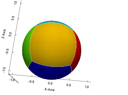
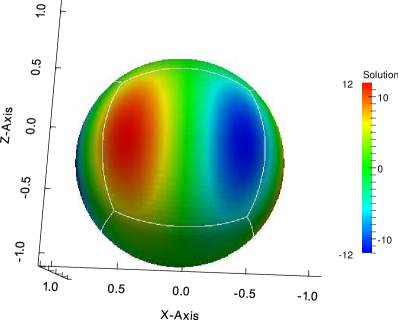
Figure 6: Sphere: Geometry and decomposition into 6 patches (left) and Solution for the Laplace-Beltrami problem (right).

The diagrams displayed in Fig. 7 show the error decay with respect to the $L_{2}$ (left) and dG (right) norms for polynomial degrees $k=1,2,3,$ and $4$. As expected by our theoretical results, we observe the full convergence rates $\mathcal{O}(h^{k+1})$ and $\mathcal{O}(h^{k})$ for the $L_{2}$ norm and the dG norm, respectively.

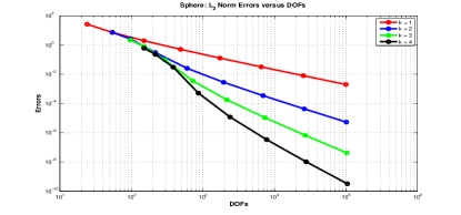
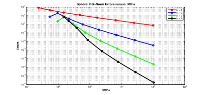
Figure 7: Sphere: Error decay in the $L_{2}$ (left) and dG (right) norms for polynomial degrees 1 to 4.

In Table 4, we compare the $L_{2}$ errors of dG IgA solutions with those produced by the corresponding continuous (standard) Galerkin (cG) IgA scheme for the polynomial degree $k=5$. In the case of smooth solutions, the dG IgA is as good as the cG counterpart. The same is true for the errors with respect to the dG norm.

Table 4: Sphere: Comparison of the cG and dG IgA error decay in the $L_{2}$ norm for $k=5$.

$k=5$	cG-IgA		dG-IgA
Dofs	$L_{2}$ error	conv. rate	$L_{2}$ error	conv. rate
216	0.168803	0	0.166582	0
294	0.0602254	1.48689	0.0599854	1.16908
486	0.00900833	2.74104	0.00898498	2.55496
1014	8.90909$\times 10^{-5}$	6.65984	8.90774$\times 10^{-5}$	6.537
2646	8.64021$\times 10^{-7}$	6.68807	8.63906$\times 10^{-7}$	6.85905
8214	1.16592$\times 10^{-8}$	6.21152	1.16582$\times 10^{-8}$	6.27626
28566	1.75119$\times 10^{-10}$	6.05699	1.75127$\times 10^{-10}$	6.06894

Torus

We now consider the closed surface

$$\Omega=\{(x,y)\in(-3,3)^{2},z\in(-1,1):\;r^{2}=z^{2}+(\sqrt{x^{2}+y^{2}}-R^{2})\}$$

that is nothing but a torus that is decomposed into 4 patches, see Fig. 8 left. The knot vectors $\Xi_{1}=\{0,0,0,0.25,0.25,0.50,0.50,0.75,0.75,1,1,1\}$ and $\Xi_{2}=\{0,0,0,1,1,1\}$ describe the NURBS used for the geometrical representation of the patches. We first consider the surface Poisson equation, also called Laplace-Beltrami equation, with the right-hand side

$$f(\phi,\theta) =r^{-2}\left[9\sin(3\phi)\cos(3\theta+\phi)\right]$$

$$-\left[(R+r\cos(\theta))^{-2}(-10\sin(3\phi)\cos(3\theta+\phi)-6\cos(3\phi)\sin(3\theta+\phi))\right]$$

$$-\left[(r(R+r\cos(\theta))^{-1})(3\sin(\theta)\sin(3\phi)\sin(3\theta+\phi))\right],$$

where $\phi=\arctan(y/x)$, $\theta=\arctan(z/(\sqrt{x^{2}+y^{2}}-R))$ , $R=2$, and $r=1$. The exact solution is given by $u=\sin(3\phi)\cos(3\theta+\phi)$, cf. also LMMT_GrossReusken:2011a . We mention that the functions $u$ and $f$ are chosen such that the zero mean compatibility condition holds. The IgA approximation to this solution is depicted in middle picture of Fig. 8.

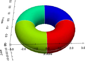
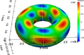
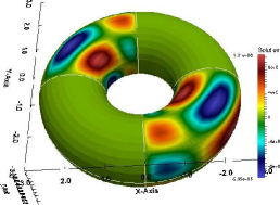
Figure 8: Torus: Geometry and decomposition into 4 patches (left), Solution for the Laplace-Beltrami problem (middle), Solution for jumping coefficents (right).

The diagrams displayed in Fig. 9 show the error decay with respect to the $L_{2}$ (left) and dG (right) norms for polynomial degrees $k=1,2,3,$ and $4$. As expected by our theoretical results, we observe the full convergence rates $\mathcal{O}(h^{k+1})$ and $\mathcal{O}(h^{k})$ for the $L_{2}$ norm and the dG norm, respectively.

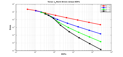
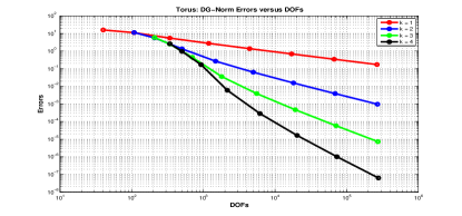
Figure 9: Torus: Error decay in the $L_{2}$ (left) and dG (right) norms for polynomial degrees 1 to 4.

In Table 5, we compare the $L_{2}$ errors of dG IgA solutions with those produced by the corresponding cG IgA scheme for the polynomial degree $k=5$. In the case of smooth solutions, the dG IgA is as good as the cG counterpart. The same is true for the errors with respect to the dG norm.

Table 5: Torus: Comparison of the cG and dG IgA error decay in the $L_{2}$ norm for $k=5$.

$k=5$	cG-IgA		dG-IgA
Dofs	$L_{2}$ error	conv. rate	$L_{2}$ error	conv. rate
504	0.0974255	0	0.0973029	0
700	0.0433491	1.1683	0.043271	1.16908
1188	0.00736935	2.55639	0.00736339	2.55496
2548	7.9296$\times 10^{-5}$	6.53814	7.92948$\times 10^{-5}$	6.537
6804	6.83083$\times 10^{-7}$	6.85904	6.83068$\times 10^{-7}$	6.85905
21460	8.8131$\times 10^{-9}$	6.27627	8.81294$\times 10^{-9}$	6.27626
75348	1.3131$\times 10^{-10}$	6.0686	1.31276$\times 10^{-10}$	6.06894

Now we consider the case when the diffusion coefficients $\alpha$ have large jumps across the boundaries of the patches in which the torus was decomposed. More precisely, we assume that the diffusion coefficient $\alpha=\alpha^{(i)}>0$ in the patch $\Omega_{i}$, $i=1,2,3,4$, where $\alpha^{(2)}=\alpha^{(4)}=1$ and $\alpha^{(1)}=\alpha^{(3)}=10^{-6}$. The patches are arranged from blue $\Omega_{1}$ to red $\Omega_{4}.$ The right-hand side $f$ is the same as given above for the case of the Laplace-Beltrami problem, i.e. for $\alpha=1.$ Now the solution is not known, but we know that the solution is smooth in the patches $\overline{\Omega_{i}}$ and has steep gradients towards $\partial\Omega_{2}$ and $\partial\Omega_{4}$, see also of Fig. 8 right. Due to our theory, we can expect full convergence rates since we have an exact representation of the geometry. Indeed, we realize the full convergence rate by choosing a fine grid as the reference solution and comparing the solutions at each refinement step against this reference solution as shown in Table 6.

Table 6: Torus: $L_{2}$ and energy norm errors with degree $k=2.$

Dofs	$L_{2}$ error	conv. rate	dG error	conv. rate
108	2.04841$\times 10^{6}$	0	8.56088$\times 10^{6}$	0
208	1.03579$\times 10^{6}$	0.98377	4.89856$\times 10^{6}$	0.805403
504	128215	3.0141	1.09244$\times 10^{6}$	2.1648
1480	15431.9	3.05458	258162	2.08121
4968	1808.17	3.09331	64084.3	2.01023
18088	213.252	3.0839	17361.8	1.88406
268840	reference	solution	reference	solution

Car

We now consider the diffusion problem on an open, free-form surface. In order to demonstrate the fact that our results are general and not limited to academic examples, we apply our methods to a CAD model representing a car shell.

The surface is composed of eight quadratic B-spline patches, shown in Fig. 10 (left). The model exhibits several small bumps in the interior of the surface and sharp corners on the boundary. In addition, the patches have varying areas and meet along curved one-dimensional (quadratic) B-spline interfaces.

We choose a constant diffusion coefficient on the whole domain and we prescribe homogeneous Dirichlet conditions along the boundary. For the right-hand side, we used a (globally defined in $\mathbb{R}^{3}$) linear function which we restricted on the surface, in order to obtain a smooth solution to our problem.

As suggested by the isogeometric paradigm, we used quadratic B-spline basis functions, forwarded on the surface, as discretization basis. We started with a coarse grid, which was $h-$refined uniformly several times, in both parametric directions.

An analytic formula for the exact solution is not available. Therefore, we have chosen a fine grid of approximately one million degrees of freedom as the reference solution. Comparing against this solution (obtained by the corresponding cG IgA method), the expected convergence rates have been observed. Table 7 contains the numeric results for the $L^{2}$ norm, obtained using either the continuous (with strong or weak imposition of Dirichlet boundaries) or dG IgA method. Apart from the observed order of convergence, the magnitude of the error agrees in all cases as well.

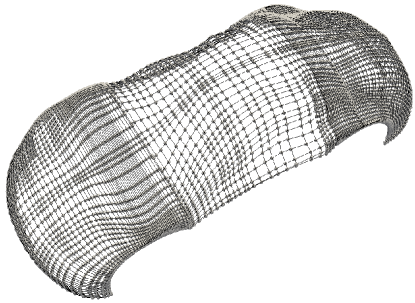
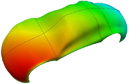
Figure 10: Car: Control points of the geometry (left), IgA solution of the Dirichlet surface diffusion problem (right). Black lines indicate patch interfaces.

$k=2$	cG IgA		Nitsche-type BCs		dG IgA
DoFs	$L_{2}$ error	rate	$L_{2}$ error	rate	$L_{2}$ error	rate
96	1.87598		1.77144		1.77029
192	1.23006	0.608922	1.19201	0.571527	1.19188	0.570749
480	0.633648	0.956971	0.623767	0.934312	0.623764	0.934161
1440	0.241842	1.38962	0.239835	1.37897	0.239835	1.37896
4896	0.0659275	1.87511	0.0655902	1.87049	0.0655902	1.87049
17952	0.0115491	2.5131	0.011502	2.5116	0.011502	2.5116
68640	0.00155178	2.89578	0.00154625	2.89504	0.00154624	2.89504
$\sim$ 268K	0.00017567	3.14298	0.000175096	3.14256	0.000175094	3.14257
$\sim$ 1M	reference	reference	reference	reference	reference	reference

Table 7: Diffusion on a car-shell model. Numerical results for continuous Galerkin IgA with strong imposition of Dirichlet boundary (cG IgA), weak imposition (Nitsche-type) and finally patch-discontinuous Galerkin (dG IgA).

4 The G+Smo C++ library

Isogeometric analysis requires seamless integration of Finite Element Analysis (FEA) and Computer-aided design (CAD) software. The existing software libraries, however, cannot be adapted easily to the rising new challenges since they have been designed and developed for different purposes. In particular, FEA codes are traditionally implemented by means of functional programming, and are focused on treating nodal shape function spaces. In CAD packages, on the other hand, the central objects are free-form curves and surfaces, defined by control points, which are realized in an object-oriented programming environment.

G+Smo is an object-oriented, template C++ library, that implements a generic concept for IGA, based on abstract classes for geometry map, discretization basis, assemblers, solvers and so on. It makes use of object polymorphism and inheritance techniques in order to support a variety of different discretization bases, namely B-spline, Bernstein, NURBS bases, hierarchical and truncated hierarchical B-spline bases of arbitrary polynomial order, and so on.

Our design allows the treatment of geometric entities such as surfaces or volumes through dimension independent code, realized by means of template meta-programming. Available features include simulations using continuous and discontinuous Galerkin approximation of PDEs, over conforming and non-conforming multi-patch computational domains. PDEs on surfaces as well as integral equations arising from elliptic boundary value problems. Boundary conditions may be imposed both strongly and weakly. In addition to advanced discretization and generation techniques, efficient solvers like multigrid iteration schemes are available. Methods for solving non-linear problems are under development. Finally, we aim to employ existing high-end libraries for large-scale parallelization.

In the following paragraphs we shall provide more details on the design and features of the library.

4.1 Description of the main modules

The library is partitioned into smaller entities, called modules. Currently, there are six (6) modules in G+Smo namely Core, Matrix, NURBS, Modeling, Input/Output and Solver modules.

The Core module is the backbone of the library. Here an abstract interface is defined for a basis, that is, a set of real-valued functions living on a parameter domain. At this level, we do not specify how these functions (or its derivatives) should be evaluated. However, a number of virtual member functions define an interface that should be implemented by derived classes of this type. Another abstract class is the geometry class. This object consists of a (still abstract) basis and a coefficient vector, and represents a patch. Note that parameter or physical dimension are not specified at this point. There are four classes directly derived from the geometry class; these are curve, surface, volume and bulk. These are parametric objects with known parameter space dimension $1,\,2,\,3$ and $4$ respectively.

Another abstract class is a function class. The interface for this class includes evaluation, derivations and other related operations. The geometry abstract class is actually deriving from the function class, demonstrating the fact that parametric geometries can be simply viewed as (vector) functions. Another interesting object is the multipatch object. CAD models are composed of many patches. Therefore, a multipatch structure is of great importance. It contains two types of information; first, geometric information, essentially a list of geometry patches. Second, topological information between the patches, that is, the adjacency graph between patch boundaries, degenerate points, and so on. Let us also mention the field class, which is the object that typically represents the solution of a PDE. A field is a mathematical scalar or vector field which is defined on a parametric patch, or multipatch object. It may be evaluated either on the parameter or physical space, as the isogeometric paradigm suggests.

The Matrix module contains all the linear algebra related infrastructure. It is based on the third party library Eigen. The main objects are dense and sparse matrices and vectors. Typical matrix decompositions such as LU, QR, SVD, and so on, are available. Furthermore, the user has also access to iterative solvers like conjugate gradient methods with different preconditioners. Finally, one can use popular high-end linear solver packages like PARADISO and SuperLU through a common interface.

The NURBS module consists of B-Splines, NURBS, Bézier of arbitrary degrees and knot-vectors, tensor-product B-splines of arbitrary spatial dimension.

The Modeling module provides data structures and geometric operations that are needed in order to prepare CAD data for analysis. It contains trimmed surfaces, boundary represented (B-rep) solids and triangle meshes. Regarding modeling operations, B-Spline fitting, smoothing of point clouds, Coon’s patches, and volume segmentation methods are available.

The Input/Output module is responsible for visualization as well as file reading and writing. For visualization, we employ Paraview or Axel (based on VTK). An important issue is file formats. Even if NURBS is an industrial standard, a variety of different formats are used in the CAD industry to exchange NURBS data. In G+Smo, we have established I/O with popular CAD formats, which include the 3DM file format of Rhinoceros 3D modeler, the X_T format of Siemens’ NX platform as well as an (exported) format used by the LS-DYNA general-purpose finite element program.

The Assembler module can already treat a number of PDE problems like convection-diffusion problems, linear elasticity, Stokes equations as well as diffusion problems on surfaces by means of continuous or discontinuous Galerkin methods, including divergence preserving discretizations for Stokes equations. Strong or weak imposition Dirichlet boundary conditions and Neumann-type conditions are provided. Boundary element IgA collocation techniques are also available.

Apart from the modules described above, there are several more which are under development. These include a hierarchical bases module, an optimization module and a triangular Bézier module.

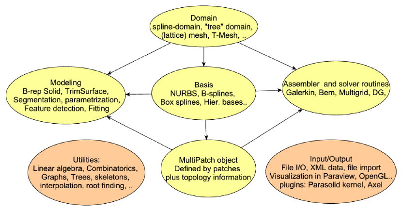
Figure 11: A diagram of the different parts in the library and their interactions

4.2 Development framework

The library uses a set of standard C++ tools in order to achieve cross-platform functionality. Some compilers that have been tested includes Microsoft’s Visual C++, Mingw32, GCC, Clang and the Intel compiler.

The main development tools used are:

• CMake cross-platform build system for configuration of the code. A small set of options are available in order to enable optional parts of the library that require external packages. Furthermore, the user is able to enable debug mode build, that disables code optimization and facilitates development, by attaching debug information in the code.

• The code is available in an SVN repository. We have chosen the continuous integration as development policy. That is, all developers commit their contributions in a mainline repository.

• Trac software management system is used for bug reporting. Additionally, we use the integrated wiki for documentation and user guidance.

• A CDASH software testing server is employed for regular compilation and testing of the mainline code. Nightly builds are executed on different platforms, as well as continuous builds after user commits. This allows to easily correct errors and ensure the quality of the library. Coverage analysis and memory checks are also performed regularly.

• The in-source documentation system Doxygen is used heavily in the code.

• A mailing list is available for communication and user support.

Regarding tools that are employed in the library:

• The C++ Standard Library is employed. This is available by default on C++ modern installations.

• The Eigen C++ Linear Algebra library is used for linear algebra operations. This library features templated coefficient type, dense and sparse matrices and vectors, typical matrix decompositions (LU, QR, SVD, ..) as well as iterative solvers and wrappers for high-end packages (SuperLU, PaStiX, SparseSuite,..).

• XML reader/writer for input/output of XML files, and other CAD formats (OFF, STL, OBJ, GeoPDEs, 3DM, Parasolid).

• Mathematical Expression Toolkit Library (ExprTk). This is an expression-tree evaluator for mathematical function expressions that allows input of functions similar to Matlab’s interface.

4.3 Additional features and extensions

Apart from the basic set of tools provided in the library, the user has the possibility to enable features that require third-party software. The following connections to external tools is provided:

• OpenNurbs library used to support Rhino’s 3DM CAD file format. This allows file exchange with standard CAD software.

• Connection to Parasolid geometric kernel. Enabling this feature allows input and output of the x_t file format. Also, the user can employ advanced modeling operations like intersection, trimming, boolean operations, and so on.

• Connection to LS-DYNA. The user can output simulation data that can be used by LS-DYNA’s Generalized element module system, for performing for instance simulations on shells.

• Connection to IPOPT nonlinear optimization library. With this feature one can use powerful interior point constrained optimization algorithms in order to perform, for instance, isogeometric shape optimization.

• MPFR library for multi-precision floating point arithmetic. With this feature critical geometric operations can be performed with arbitrary precision, therefore guaranteeing a verified result.

• Graphical interface, interaction and display using Axel modeler.

4.4 Plugins for third-party platforms

Finally, there are currently two plugins under development. The plugins allow third-party software to employ and exchange data with G+Smo.

• Axel Modeler is an open-source spline modeling package based on Qt and VTK. Our plugin allows to use G+Smo within this graphical interface, and provides user interaction (e.g. control point editing) and display.

• A Matlab interface is under development. This allows to use operations available in G+Smo within Matlab.

Acknowledgement. This research was supported by the Research Network “Geometry + Simulation” (NFN S117), funded by the Austrian Science Fund (FWF).

References

- [1] R. A. Adams and J. J. F. Fournier. Sobolev Spaces. Pure and Applied Mathematics 140, Elsevier/Academic Press, second edition, 2008.
- [2] P. Antonietti, A. Dedner, P. Madhavan, S. Stangalino, B. Stinner, and M. Veran. High order discontinuous Galerkin methods on surfaces, 2014. arXiv:1402.3428.
- [3] T. Apel and F. Milde. Comparison of several mesh refinement strategies near edges. Commun. Numer. Meth. Engng, 12:373–381, 1996.
- [4] T. Apel, A.-M. Sändig, and J. R. Whiteman. Graded mesh refinement and error estimates for finite element solutions of elliptic boundary value problems in non-smooth domains. Math. Meth. Appl. Sci., 19(30):63–85, 1996.
- [5] Y. Bazilevs, L. Beirão da Veiga, J. Cottrell, T. Hughes, and G. Sangalli. Isogeometric analysis: Approximation, stability and error estimates for -refined meshes. Comput. Methods Appl. Mech. Engrg., 194:4135–4195, 2006.
- [6] L. Beirão da Veiga, A. Buffa, J. Rivas, and G. Sangalli. Some estimates for h–p–k-refinement in isogeometric analysis. Numerische Mathematik, 118(2):271–305, 2011.
- [7] L. Beirão da Veiga, D. Cho, and G. Sangalli. Anisotropic NURBS approximation in isogeometric analysis. Comput. Methods Appl. Mech. Engrg., 209–212(0):1 – 11, 2012.
- [8] J. Cottrell, T. Hughes, and Y. Bazilevs. Isogeometric analysis: Toward Integration of CAD and FEA. John Wiley & Sons, Chichester, 2009.
- [9] L. Dede and A. Quarteroni. Isogeometric analyis for second order partial differential equations on surfaces. MATHICSE Report 36.2012, Politecnico di Milano, 2012.
- [10] A. Dedner and P. Madhavan. Adaptive discontinuous Galerkin methods on surfaces. arXiv, 2014. http://arxiv.org/abs/1402.1185 and accepted for publication in Numerische Mathematik.
- [11] A. Dedner, P. Madhavan, and B. Stinner. Analysis of the discontinuous Galerkin method for elliptic problems on surfaces. IMA J. Numer. Anal., 33(3):952–973, 2013.
- [12] D. A. Di Pietro and A. Ern. Analysis of a discontinuous Galerkin method for heterogeneous diffusion problems with low-regularity solutions. Numerical Methods for Partial Differential Equations, 28(4):1161–1177, 2012.
- [13] D. A. Di Pietro and A. Ern. Mathematical Aspects of Discontinuous Galerkin Methods, volume 69 of Mathématiques et Applications. Springer-Verlag, 2012.
- [14] M. Dryja. On discontinuous Galerkin methods for elliptic problems with discontinuous coeffcients. Comput. Meth. Appl. Math., 3:76–85, 2003.
- [15] G. Dziuk. Finite elements for the Beltrami operator on arbitrary surfaces. In S. Hildebrandt and R. Leis, editors, Partial Differential Equations and Calculus of Variations, volume 1357 of Lecture Notes in Mathematics, pages 142–155. Springer, 1988.
- [16] G. Dziuk and C. Elliott. Finite elements on evolving surfaces. IMA J. Num. Anal., 27(2):262–292, 2007.
- [17] G. Dziuk and C. Elliott. Surface finite elements for parabolic equations. J. Comput. Math., 25(4):385–407, 2007.
- [18] G. Dziuk and C. Elliott. Finite element methods for surface PDEs. Acta Numerica, 22:289–396, 2013.
- [19] L. C. Evans. Partial Differential Equestions, volume 19 of Graduate Studies in Mathematics. American Mathematical Society, 1st edition, 1998.
- [20] P. Grisvard. Elliptic problems in nonsmooth domains. Monographs and studies in mathematics. Pitman Advanced Pub. Program, 1985.
- [21] P. Grisvard. Elliptic Problems in Nonsmooth Domains. SIAM, 2011.
- [22] S. Gross and A. Reusken. Numerical Methods for Two-phase Incompressible Flows. Springer Series in Computational Mathematics. Springer, 2011.
- [23] T. Hughes, J. Cottrell, and Y. Bazilevs. Isogeometric analysis: CAD, finite elements, NURBS, exact geometry and mesh refinement. Comput. Methods Appl. Mech. Engrg., 194:4135–4195, 2005.
- [24] J. W. Jeong, H.-S. Oh, S. Kang, and H. Kim. Mapping techniques for isogeometric analysis of elliptic boundary value problems containing singularities. Comput. Methods Appl. Mech. Engrg., 254:334 – 352, 2013.
- [25] R. B. Kellogg. On the Poisson equation with intersecting interfaces. Appl. Anal., 4:101–129, 1975.
- [26] S. Kleiss, B. Juettler, and W. Zulehner. Enhancing isogeometric analysis by finite element-based local refinement strategies. Comput. Methods Appl. Mech. Engrg., 2012.
- [27] U. Langer, A. Mantzaflaris, S. E. Moore, and I. Toulopoulos. Mesh grading in isogeometric analysis for solving elliptic boundary value problems with singular solutions. in preperation, 2014.
- [28] U. Langer and S. Moore. Discontinuous Galerkin isogeometric analysis of elliptic PDEs on surfaces. NFN Technical Report 12, Johannes Kepler University Linz, NFN Geometry and Simulation, Linz, 2014. http://arxiv.org/abs/1402.1185 and accepted for publication in the DD22 proceedings.
- [29] U. Langer and I. Toulopoulos. Analysis of multipatch discontinuous Galerkin IgA dpproximations to elliptic boundary value problems. RICAM Reports 2014-08, Johann Radon Institute for Computational and Applied Mathematics, Austrian Academy of Sciences, Linz, 2014. http://arxiv.org/abs/1408.0182.
- [30] A. Mantzaflaris and B. Jüttler. Exploring matrix generation strategies in isogeometric analysis. In M. Floater, T. Lyche, M.-L. Mazure, K. Mørken, and L. Schumaker, editors, Mathematical Methods for Curves and Surfaces, volume 8177 of LNCS, pages 364–382. Springer, 2014.
- [31] A. Mantzaflaris and B. Jüttler. Integration by interpolation and look-up for Galerkin-based isogeometric analysis. Comp. Methods Appl. Mech. Engrg., 284:373 – 400, 2015.
- [32] L. Oganesjan and L. Ruchovetz. Variational difference methods for the solution of elliptic equations. Isdatelstvo Akademi Nank Armjanskoj SSR, Erevan, 1979. (in Russian).
- [33] H.-S. Oh, H. Kim, and J. W. Jeong. Enriched isogeometric analysis of elliptic boundary value problems in domains with cracks and/or corners. Int. J. Numer. Meth. Engng, 97(3):149–180, 2014.
- [34] B. Rivière. Discontinuous Galerkin Methods for Solving Elliptic and Parabolic Equations: Theory and Implementation. SIAM, Philadelphia, 2008.
- [35] F. Zhang, Y. Xu, and F. Chen. Discontinuous Galerkin methods for isogeometric analysis for elliptic equations on surfaces. http://staff.ustc.edu.cn/ yxu/paper/IGA-DG.pdf, 2014.