CHEMISTRY OF THE MOST METAL-POOR STARS IN THE BULGE AND THE $z\gtrsim 10$ UNIVERSE

Abstract

Metal-poor stars in the Milky Way are local relics of the epoch of the first stars and the first galaxies. However, a low metallicity does not prove that a star formed in this ancient era, as metal-poor stars form over a range of redshift in different environments. Theoretical models of Milky Way formation have shown that at constant metallicity, the oldest stars are those closest to the center of the Galaxy on the most tightly-bound orbits. For that reason, the most metal-poor stars in the bulge of the Milky Way provide excellent tracers of the chemistry of the high-redshift universe. We report the dynamics and detailed chemical abundances of three stars in the bulge with $\mathrm{[Fe/H]}\lesssim-2.7$, two of which are the most metal-poor stars in the bulge in the literature. We find that with the exception of scandium, all three stars follow the abundance trends identified previously for metal-poor halo stars. These three stars have the lowest [Sc II/Fe] abundances yet seen in $\alpha$-enhanced giant stars in the Galaxy. Moreover, all three stars are outliers in the otherwise tight [Sc II/Fe]–[Ti II/Fe] relation observed among metal-poor halo stars. Theoretical models predict that there is a 30% chance that at least one of these stars formed at $z\gtrsim 15$, while there is a 70% chance that at least one formed at $10\lesssim\!z\!\lesssim 15$. These observations imply that by $z\sim 10$, the progenitor galaxies of the Milky Way had both reached $\mathrm{[Fe/H]}\sim-3.0$ and established the abundance pattern observed in extremely metal-poor stars.

1. Introduction

The first stars are thought to form at $z\gtrsim 15$, with the first galaxies following at $z\sim 10$ (e.g., Bromm et al., 1999; Abel et al., 2002; Bromm & Yoshida, 2011). The chemical abundances of these first galaxies are unknown. If those abundances could be measured, then they would constrain the properties of metal-free Population III stars, the early chemical evolution of galaxies, and the reionization of the universe. Metal-poor stars in the Milky Way provide a local link to this high-redshift universe through the elemental abundances of their photospheres.

As the number of known metal-poor stars with detailed chemical abundance measurements has grown, it has become possible to homogeneously analyze large samples to search for subtle trends (e.g., Cayrel et al., 2004; Bonifacio et al., 2009; Norris et al., 2013a, b; Yong et al., 2013a, b; Roederer et al., 2014). It is tempting to assert that these metal-poor stars in the halo are the direct descendants of the first stars. This is not necessarily the case though, as metal-poor stars form over a range of redshift in halos of varying mass and environment. Likewise, stars at a given redshift form with a range of metallicity. The examination of other properties beyond metallicity are therefore necessary to identify the stars in the Milky Way that formed at the highest redshifts.

Tumlinson (2010) showed that because galaxies form from the inside-out, the oldest stars at a given metallicity are found near the center of a halo on the most tightly-bound orbits. Indeed, near the center of a Milky Way-analog a large fraction of stars with $-3\lesssim\mathrm{[Fe/H]}\lesssim-2$ formed at $z\gtrsim 6$, while 20–40% of stars with $-4\lesssim\mathrm{[Fe/H]}\lesssim-3$ formed at $10\lesssim z\lesssim 15$. Consequently, the metal-poor stellar population in the inner few kpc of the Galaxy—the bulge—is the best place to search for truly ancient stars, including low-mass Population III stars that may have survived to the present day.

Large-scale spectroscopic surveys of the bulge have shown that while metal-poor stars in the bulge are quite rare, they do exist. The Abundances and Radial Velocity Galactic Origins (ARGOS) survey of Freeman et al. (2013) and Ness et al. (2013) identified 16 stars with $\mathrm{[Fe/H]}\lesssim-2.0$ in a sample of 14,150 stars within 3.5 kpc of the Galactic center. The most metal-poor star in their sample has $\mathrm{[Fe/H]}\approx-2.6$. As part of the third phase of the Sloan Digital Sky Survey, the Apache Point Observatory Galactic Evolution Experiment (APOGEE) collected $H$-band spectra for 2,403 giants stars in outer bulge fields and identified two stars with $\mathrm{[Fe/H]}\approx-2.1$ (García Pérez et al., 2013).

Ground-based objective prism surveys for metal-poor stars in the bulge are impractical due to crowding and strong absolute and differential reddening. For this reason, searches for metal-poor stars have historically avoided the inner regions of our own Galaxy. Recently though, the Extremely Metal-poor BuLge stars with AAOmega (EMBLA) survey has successfully used narrow-band SkyMapper $v$-band photometry (Bessell et al., 2011) in the Ca II H & K region to pre-select candidate metal-poor stars for follow-up spectroscopy. In a sample of more than 8,600 stars, Howes et al. (2014) found in excess of 300 stars with $\mathrm{[Fe/H]}\lesssim-2.0$—including four stars with $-2.7\lesssim\mathrm{[Fe/H]}\lesssim-2.5$. Still, strong absolute and significant differential reddening limits the efficiency of near UV based selections for metal-poor stars in the bulge and restricts their applicability to outer-bulge regions.

In Schlaufman & Casey (2014), we described a new technique to identify candidate metal-poor stars using only near-infrared 2MASS and mid-infrared WISE photometry (Skrutskie et al., 2006; Wright et al., 2010; Mainzer et al., 2011). Our infrared selection is well suited to a search for metal-poor stars in the bulge, as it is minimally affected by crowding or reddening. We found that more than 20% of the candidates selected with our infrared selection are genuine very metal-poor (VMP) stars with $-3.0\lesssim\mathrm{[Fe/H]}\lesssim-2.0$. Another 2% of our candidates are genuine extremely metal-poor (EMP) stars with $-4.0\lesssim\mathrm{[Fe/H]}\lesssim-3.0$. In a sample of 90 metal-poor candidates—selected with only an apparent magnitude cut to be high in the sky from Las Campanas in the first half of the year—we identified three stars with $-3.1\lesssim\mathrm{[Fe/H]}\lesssim-2.7$ within 4 kpc of the Galactic center. Two of these stars are the most metal-poor stars in bulge in the literature, while the third is comparable to the most metal-poor star from Howes et al. (2014).

Because these stars are both tightly bound to the Galaxy and very metal-poor, they are likely to be among the most ancient stars identified to this point. For that reason, their detailed abundances provide clues to the chemistry of the first galaxies in the $z\gtrsim 10$ universe, beyond those already identified in more metal-poor halo stars. These stars all have apparent magnitudes $V\lesssim 13$, making them unusually bright for stars at the distance of the bulge. Their bright apparent magnitudes enable a very telescope-time efficient exploration of the $z\gtrsim 10$ Universe. We describe the collection of the data we will subsequently analyze in Section 2. We detail the determination of distances and orbital properties, stellar parameters, and chemical abundances of these three stars in Section 3. We discuss our results and their implications in Section 4, and we summarize our findings in Section 5.

2. Data Collection

We initially selected these stars as candidates according to criteria (1)–(4) from Section 2 of Schlaufman & Casey (2014): $0.45\leq J-H\leq 0.6$, $W3>8$, $-0.04\leq W1-W2\leq 0.04$, and $J-W2>0.5$. We give astrometry and photometry for each star in Table 1. We confirmed their metal-poor nature using low-resolution spectroscopy from Gemini South/GMOS-S (Hook et al., 2004) in service mode during March and April of 2014. Our Gemini South/GMOS-S follow-up spectroscopy was not focused on candidates in the bulge, so the discovery of these stars in the bulge was not predetermined by our survey strategy. We used the Magellan Inamori Kyocera Echelle (MIKE) spectrograph (Bernstein et al., 2003) on the Clay Telescope at Las Campanas Observatory on 2014 June 21–22 to obtain high-resolution, high signal-to-noise (S/N) spectra suitable for a detailed chemical abundance analysis. We observed all three stars in 0$\farcs$5 seeing at airmass $<\!\!1.01$ with exposure times in the range 390–590 seconds. The total exposure time for all three sources combined was less than 24 minutes. Including overheads, our Magellan/MIKE observations for all three stars were completed in about 30 minutes. We used the 0$\farcs$7 slit and the standard blue and red grating azimuths, yielding spectra between 332 nm and 915 nm with resolution $R\approx 41,\!000$ in the blue and $R\approx 35,\!000$ in the red. The resultant spectra have S/N $\gtrsim 50$ pixel^-1 at 400 nm and S/N $\gtrsim 100$ pixel^-1 at 600 nm.

To obtain proper motions for each star, we cross-matched with both the UCAC4 and SPM4 proper motion catalogs using TOPCAT(Zacharias et al., 2013; Girard et al., 2011; Taylor, 2005). We list both sets of proper motions for our sample in Table 2.

3. Analysis

We reduced the spectra using the CarPy software package (Kelson, 2003; Kelson et al., 2014). We continuum-normalized individual echelle orders using spline functions before joining them to form a single contiguous spectrum. We estimate line-of-sight radial velocities by cross-correlating each spectrum with a normalized rest-frame spectrum of the well-studied metal-poor giant star HD 122563. We use the measured radial velocities to place the spectra in the rest-frame of the star.

3.1. Distances & Dynamics

To determine the distances between the sun and each star in our sample, we use the scaling relation

$$L/L_{\odot} = (R/R_{\odot})^{2}(T_{\mathrm{eff}}/T_{\mathrm{eff,\odot}})^{4},$$ (1)

$$= (M/M_{\odot})(g/g_{\odot})^{-1}(T_{\mathrm{eff}}/T_{\mathrm{eff,\odot}})^{4}.$$ (2)

Taking their characteristic mass as $0.8~{}M_{\odot}$, the bolometric luminosity $L$ of our stars can be approximated as

$$\log{\left(L/L_{\odot}\right)} = \log{0.8}-(\log{g}-4.44)+4\log{\left(T_{\mathrm{eff}}/5777~{}\mathrm{K}\right)}.$$

We then use Equation LABEL:eq-lum and the stellar parameters from Schlaufman & Casey (2014) listed in Table 3 to determine $L$. We use a 10 Gyr, ${\mathrm{[Fe/H]}=-2.5}$, and ${[\alpha/{\rm Fe}]=+0.4}$ Dartmouth isochrone to convert $L$ into an absolute $W1$-band magnitude $M_{W1}$ (Dotter et al., 2008). Given the available photometry, $W1$ is least affected by extinction. We de-redden the observed $W1$ magnitudes using the Schlegel et al. (1998) dust maps as updated in Schlafly & Finkbeiner (2011) along with the Indebetouw et al. (2005) infrared extinction law. The distance modulus $W1-M_{W1}$ then yields $d_{\odot}$, the approximate distance of each star from the sun. Assuming the distance to the Galactic center is $R_{0}=8.2\pm 0.4$ kpc (e.g., Bovy et al., 2009), we can then compute $d_{\mathrm{gc}}$, the approximate distance of each star from the Galactic center. We perform a Monte Carlo simulation to account for the random observational uncertainties in $W1$, $A_{W1}$, $T_{\mathrm{eff}}$, $\log{g}$, and $R_{0}$. We sample 10,000 realizations from the uncertainty distributions for each quantity and compute $d_{\odot}$ and $d_{\mathrm{gc}}$ for each realization. We give both distance estimates and their random uncertainties in the first two columns of Table 4. All three stars have $d_{\mathrm{gc}}\lesssim 4$ kpc.

We compute the Galactic orbits of each star in our sample using the galpy code, with initial conditions set by the observed heliocentric radial velocities and proper motions in Table 2 and estimated $d_{\odot}$ values from Table 4. Following Bovy et al. (2012), we model the Milky Way’s potential as the superposition of a Miyamoto-Nagai disk with a radial scale length of 4 kpc and a vertical scale height of 300 pc, a Hernquist bulge with a scale radius of 600 pc, and a Navarro-Frenk-White halo with a scale length of 36 kpc (Miyamoto & Nagai, 1975; Hernquist, 1990; Navarro et al., 1996). We assume that the Miyamoto-Nagai disk, the Hernquist bulge, and the Navarro-Frenk-White halo respectively contribute 60%, 5%, and 35% of the rotational support at the solar circle. We integrate the orbits for 200 orbital periods and derive the pericenters $r_{\mathrm{peri}}$, apocenters $r_{\mathrm{ap}}$, and eccentricities $e$. We perform a Monte Carlo simulation to account for the random observational uncertainties in $d_{\odot}$, $v_{\mathrm{hel}}$, $\mu_{\alpha}\cos{\delta}$, and $\mu_{\delta}$. We sample 1,000 realizations from the uncertainty distributions for each quantity and use those data as input to an orbital integration. In an attempt to quantify the systematic uncertainties that result from the input proper motion measurements, we include in Table 4 orbital properties and uncertainties estimated using both UCAC4 and SPM4 proper motions.

3.2. Stellar Parameters

We estimate stellar parameters by classical excitation and ionization balance using unblended Fe I and Fe II lines. Following the process described in Casey (2014), we measure equivalent widths of individual absorption lines from the rest-frame spectra by fitting Gaussian profiles. We visually inspect all lines for quality, and discard blended or low-significance measurements. For these analyses, we assume transitions are in local thermodynamic equilibrium (LTE) and employ the plane-parallel 1D $\alpha$-enhanced model atmospheres from Castelli & Kurucz (2004). We use the atomic data compiled by Roederer et al. (2010), the Asplund et al. (2009) solar chemical composition, and the February 2013 version of MOOG to calculate line abundances and synthesize spectra (Sneden, 1973; Sobeck et al., 2011). We require four conditions to be simultaneously met for a converged set of stellar parameters: zero trend in Fe I line abundance with excitation potential, zero trend in Fe I line abundances with reduced equivalent width, equal mean Fe I and Fe II abundances, and that the mean [Fe I/H] abundance must match the input model atmosphere abundance [M/H]. In practice we accepted solutions where the slopes had magnitudes less than $10^{-3}$ and the absolute abundance differences were less than $10^{-2}$ dex. Our estimated stellar parameters are provided in Table 3.

To verify our spectroscopically-derived effective temperatures, we calculate effective temperatures using color–temperature relations for 2MASS $J-K_{s}$ and APASS/2MASS $V-K_{s}$ colors. We use the Schlegel et al. (1998) dust maps as updated by Schlafly & Finkbeiner (2011) to account for reddening in both colors. However, we find that our photometric temperatures are as much as $600$ K hotter than our spectroscopically-derived quantities. To explore the reason for this discrepancy, we also estimate effective temperatures by comparing the observed Balmer lines with synthetic spectra from Barklem & Piskunov (2003). Our analysis of the H-$\beta$ profile suggests effective temperatures between $4600$ K and 4800 K for all three stars, in excellent agreement with our excitation-ionization balance measurements. As we show qualitatively in Figure 1, our observed spectra are very similar to the well-studied metal-poor giant star HD 122563. Given our independent effective temperature estimates, and since HD 122563 is a red giant branch star with $T_{\mathrm{eff}}=4590$ K, $\log{g}=1.61$, and $\mathrm{[M/H]}=-2.64$ (Jofré et al., 2014), we are confident in our derived spectroscopic effective temperatures. Moreover, we observe repeated saturated interstellar Na I D absorption lines in our data. These lines are indicative of multiple optically-thick gas clouds along the line-of-sight, each with distinct velocities. For these reasons, we assert that the discrepancy between photometric and spectroscopic temperatures is likely due to poorly-characterized reddening in the outer bulge region. Given the spectral resolution and S/N ratios of our data, we estimate that the uncertainties in our spectroscopically-derived stellar parameters are about $100$ K in $T_{\rm eff}$, 0.2 dex in $\log{g}$, 0.1 dex in [Fe/H], and 0.1 km s^-1 in microturbulence ($\xi$).

We note that our stellar parameters ($T_{\rm eff}$, $\log{g}$, [Fe/H], $\xi$) would change if we used different model atmospheres or included a proper treatment of non-LTE effects. For metal-poor giants, the non-LTE treatment would increase the mean Fe I line abundance by about 0.1 dex and result in higher surface gravities for a given effective temperature. As an example, Jofré et al. (2014) reports a slightly cooler temperature and higher surface gravity for HD 122563 than we find for our three stars. However, in that study $T_{\rm eff}$ and $\log{g}$ were not derived by excitation and ionization equilibrium. Instead, they were fixed by bolometric temperature and angular diameter measurements from Creevey et al. (2012). With the stellar parameters fixed, Jofré et al. (2014) noted that HD 122563 showed the largest abundance imbalance of Fe I and Fe II lines in their sample. This indicates the the application of the equilibrium method in LTE tends towards a different set of stellar parameters. In Figure 2 we plot our stars alongside giant star (i.e., $\log{g}\lesssim 3.0$) comparison samples from Yong et al. (2013a) and Roederer et al. (2014). Although these authors estimated surface gravities directly from isochrones, our stellar parameters are comparable to their determinations. Consequently, we are confident of our stellar parameter estimates.

3.3. Detailed Abundances

Our high-resolution, high S/N Magellan/MIKE spectra allow us to measure the abundances of many light, odd-Z, $\alpha$, Fe-peak, and neutron-capture elements. For most elements, we determine individual line abundances from the measured equivalent widths of clean, unblended atomic lines. We take a synthesis approach for molecular features (e.g., CH), doublets (e.g., Li), or atomic transitions with significant hyperfine structure and/or isotopic splitting (namely Sc, V, Mn, Co, Cu, Ba, La, and Eu). We use molecular data (CH) from Masseron et al. (2014). Our hyperfine structure and isotopic splitting data come from Kurucz & Bell (1995) for Sc, V, Mn, Co, and Cu, from Biémont et al. (1999) for Ba, and from Lawler et al. (2001a, b) for La and Eu. We assume standard solar system isotopic fractions as collated by Anders & Grevesse (1989). We report our equivalent width measurements in Table 5 and our derived abundances in Table 6.

We estimate lithium abundances through synthesis of the Li doublet at $\lambda$6707. This feature is quite weak in our spectra. However, the abundances we obtain are typical for stars at the tip of the red giant branch. We synthesize the $G$-band molecular feature at $\lambda$4323 to estimate carbon abundances. None of our stars are carbon enhanced by the Beers & Christlieb (2005) definition of [C/Fe] $\gtrsim+1.0$. On the other hand, one of our stars is carbon enhanced by the Aoki et al. (2007) definition that takes stellar evolutionary effects into account. In either case, there is not much carbon present in the photospheres of our stars—[C/Fe] ranges from $-0.61$ in J183713-314109 to $+0.15$ in J181503-375120. We measure potassium abundances from equivalent widths of the strong K I transitions at $\lambda$7664 and $\lambda$7698. Given the radial velocities of our targets, these K I lines were mostly separated from the telluric A-band feature near $\lambda$7600. We detected Na I in all three stars and derive abundances from the strong $\lambda$5889 and $\lambda$5895 transitions. We measure Al I from the $\lambda$3961 feature.

All three stars appear $\alpha$-enhanced (Mg, Ti, Si, and Ca). On average, the $\alpha$-element abundances of these three metal-poor stars in the bulge are similar to those observed in large samples of halo metal-poor giant stars (e.g., Cayrel et al., 2004; Yong et al., 2013a; Roederer et al., 2014). [Mg/Fe] varies between $+0.46$ and $+0.57$, while [Ca/Fe] changes marginally from $+0.41$ to $+0.47$. However, in all stars we find that [Ti I/Fe] and [Ti II/Fe] are slightly lower than the other $\alpha$-elements, between [Ti/Fe]$=+0.22$ and $+0.29$ (Figure 3). In all stars, the mean abundances of neutral and ionized Ti transitions agree within 0.03–0.08 dex. We measure [Si I/Fe] abundances from the $\lambda$3905 transition, yielding [Si I/Fe] abundance ratios between $+0.71$ and $+0.86$.

There are a large number of Fe-peak transitions available in our spectra: Sc II, V I, Cr I & Cr II, Mn I, Co I, Ni I, Cu I, and Zn I. While Sc, V, Cr, Mn, Co, Ni, and Zn are clearly measurable in all stars from multiple unblended lines, we do not detect Cu I in J155730-293922 or J183713-314109. Instead, we provide upper limits for Cu I from the $\lambda$5105 transition. We also report a low-significance detection of Cu I in J181503-375120 of [Cu I/Fe] $=-0.51$. Our Fe-peak abundance ratios generally follow the mean halo abundance trends observed by other authors in giant stars of similar metallicity (e.g., Cayrel et al., 2004; Yong et al., 2013a; Roederer et al., 2014). We find that [Si I/Fe], [Sc II/Fe], and [Mn I/Fe] abundances are at the extremes of the abundance distribution observed in halo metal-poor giant stars. We show this in Figure 5 and explore possible explanations for these observations in Section 4.

We measure elemental abundances from the first (Sr and Y) and second (Ba) neutron-capture peaks. We do not detect Eu or La in our targets, and therefore we report upper limits for these elements in Table 6. Sr and Y have a common nucleosynthetic pathway, and we observe comparable abundance ratios for these elements in all three stars. As we show in Figure 4, all of our measured neutron-capture abundances are indistinguishable from the abundances observed in halo metal-poor giant stars (Yong et al., 2013a; Roederer et al., 2014).

The uncertainties in chemical abundances are dominated by systematics, principally due to the uncertainties in determining stellar parameters. We vary the stellar parameters of each star by the estimated uncertainties and calculate the resulting change in abundances. We give the sign and magnitude of these effects in Table 7, along with the quadrature sum of systematic uncertainties. Due to a lack of lines for some elements, we adopt a minimum random uncertainty of 0.1 dex. We estimate total uncertainties as the quadrature sum of random and systematic uncertainties, which we list in Table 7. For uncertainties in [X/Fe] abundance ratios (e.g., as shown in Figures 3–5), we adopt the quadrature sum of the total uncertainties in [X/H] and [Fe I/H].

4. Discussion

Our initial survey was not targeted at the bulge, so we are observing all three stars at random orbital phases. Since a star on a radial orbit spends most of its orbit near apocenter, there is a strong prior that we are observing all three stars close to apocenter. Our estimated Galactocentric distances and orbital parameters for the three stars listed in Table 4 securely place J155730-293922 and J183713-314109 in the bulge on tightly bound orbits. In both cases, the currently-observed Galactocentric distances are consistent with the idea that both stars are near apocenter. At the same time, the differences in proper motion reported by UCAC4 and SPM4 deviate by up to 3-$\sigma$. It seems clear that the quoted random proper motion uncertainties are not representative of the total uncertainties including the contribution from systematics. Both stars have $V\lesssim 13$ and have had their proper motions matched to the correct 2MASS sources, so the discrepancy is not due to faintness or misidentification. Nevertheless, the range in proper motions reported by UCAC4 and SPM4 should be an approximation of the effect of the unreported systematic uncertainties. Since both UCAC4 and SPM4 place J155730-293922 and J183713-314109 on tightly bound orbits, there is no reason to reject the idea that they are indeed tightly bound. We therefore argue that since J155730-293922 and J183713-314109 are metal-poor, located near the center of the Galaxy, and on tightly bound orbits, they are likely to be truly ancient stars according to the analysis described in Tumlinson (2010).

On the other hand, the orbital parameters listed in Table 4 for the star J181503-375120 suggest that it may be a halo star on a very eccentric orbit. Both UCAC4 and SPM4 agree that $\mu_{\alpha}\cos{\delta}\approx 20$ mas yr^-1 with high significance, indicating a substantial transverse velocity at $9.0_{-2.2}^{+2.8}$ kpc. The problem with that scenario is that J181503-375120 would spend only a tiny fraction of its orbit near where it is observed today, and we are therefore observing it at a special time. There are two possible interpretations of this observation. The first is that both UCAC4 and SPM4 have somehow overestimated the $\mu_{\alpha}\cos{\delta}$ proper motion of J181503-375120. This cannot easily be rejected. Though the UCAC4 and SPM4 proper motion measurements were produced independently, they both used the same blue SPM plates for their first epoch astrometry. In that case, the apparently large proper motion of J181503-375120 could be the result of an issue with the same blue SPM plate. Moreover, both UCAC4 and SPM4 may be subject to residual systematic uncertainties at the level of 10 mas yr^-1. The second interpretation is that J181503-375120 is genuinely on a very eccentric orbit that takes it from the bulge all the way to the edge of the Local Group. Though we cannot reject the latter hypothesis, we suspect that the former is a better explanation. Nevertheless, the proper motion of J181503-375120 merits further attention. If its parallax is measured and its proper motion confirmed by Gaia, then it could be a hypervelocity star that has been ejected from the Galactic center by a three-body interaction involving the Milky Way’s supermassive black hole. In any case, J181503-375120 is currently located near the center of the Galaxy.

Since all three stars in our sample are old, one might wonder if the orbits we observe today might be significantly different from their orbits at higher redshift. Even though we will argue that our stars formed at $z\sim 10$, they were likely accreted by the Milky Way more recently. Tumlinson (2010) found that even metal-poor stars that formed at $z\sim 10$ are not typically accreted by a Milky Way analog until $z\sim 3$. Wang et al. (2011) showed that in the absence of a major merger, inside of 2 kpc Milky Way-analog dark matter halos have accreted more than 75% of their $z=0$ mass by $z\sim 3$. The Milky Way is not likely to have had a major merger in that interval, as its disk is quite old and its bulge appears to be a psuedobulge best explained by secular disk instabilities (e.g., Aumer & Binney, 2009; Schönrich & Binney, 2009; Kormendy & Kennicutt, 2004; Howard et al., 2009). The fact that the mass enclosed by the orbits of of our stars does not change much since they likely entered the Milky Way’s dark matter halo suggests that their orbits should not have changed significantly. The impact of merger activity would be to cause the outward diffusion of stellar orbits anyway, so in that situation the orbits of our stars would have been even more tightly bound in the past. This would not qualitatively effect our interpretation of their abundances.

The inside-out formation of the Milky Way suggests that in the inner few kpc of the Galaxy, about 10% of stars with $\mathrm{[Fe/H]}\lesssim-3.0$ formed at $z\gtrsim 15$ (Tumlinson, 2010). Another 20–40% of stars in the range $-4.0\lesssim\mathrm{[Fe/H]}\lesssim-3.0$ formed at $10\lesssim z\lesssim 15$. All three of our stars are currently in the inner Galaxy, while the kinematics of two of the three place them on tightly bound orbits. The probability $P_{15}$ that at least one of our stars formed at $z\gtrsim 15$ is 1 minus the probability that none of them formed at $z\gtrsim 15$: $P_{15}=1-0.9^{3}\approx 0.3$. Likewise, the probability $P_{10}$ that at least one of our stars formed at $z\gtrsim 10$ is $P_{10}=1-0.7^{3}\approx 0.7$. In other words, there is 30% chance that at least one of these three stars formed at $z\gtrsim 15$ and a 70% chance that at least one star formed at $10\lesssim z\lesssim 15$. If we apply the Tumlinson (2010) analysis only to J155730-293922 and J183713-314109, then $P_{15}\approx 0.2$ and $P_{10}\approx 0.5$. Even though these stars are not the most metal-poor stars known, the combination of their low metallicity and tightly-bound orbits suggests that they may be among the most ancient stars with detailed chemical abundance measurements.

In this scenario, our derived chemical abundances are indicative of the chemical abundances of the progenitor galaxies of the Milky Way during the epoch of the first galaxies. Generally, we find that our abundance ratios are near the mean of abundance distributions observed in halo metal-poor giant stars (Cayrel et al., 2004; Yong et al., 2013a; Roederer et al., 2014). Si, Sc and Mn are exceptions though, which we discuss below. Based on four metal-poor bulge stars with $-2.7\lesssim\mathrm{[Fe/H]}\lesssim-2.5$ from the EMBLA survey, Howes et al. (2014) reached a similar conclusion: bulge metal-poor stars have a similar abundance pattern to halo metal-poor stars. They also noted large scatter in [Mg I/Fe] from $-0.07$ to $+0.62$ in just four stars, with one star overabundant in [Ti II/Fe] to the level of $+0.84$. We find very little variance in [Mg I/Fe], ranging from $+0.46$ to $+0.57$. None of our stars are overabundant in either [Ti I/Fe], [Ti II/Fe], or any other $\alpha$-elements. In fact, we find that [Ti I/Fe] and [Ti II/Fe] are about $0.15$ dex below the abundances of other $\alpha$-elements.

Our stars appear near the extremes of the silicon abundance distribution observed in halo metal-poor giant stars (e.g., Cayrel et al., 2004; Yong et al., 2013a; Roederer et al., 2014). This is likely due to their low surface gravities and temperatures though. Bonifacio et al. (2009) found that giants exhibited higher [Si/Fe] abundance ratios than dwarfs by about 0.2 dex. Similarly, cool stars usually appear to have high silicon (Preston et al., 2006; Lai et al., 2008; Yong et al., 2013a). Given these two effects, the slightly higher [Si/Fe] abundance ratios we find can most likely be attributed to a combination of low surface gravity and cool temperatures. Indeed, when we consider [Si/Fe] in giant stars ($\log{g}<3$) in the Roederer et al. (2014) sample, our [Si/Fe] ratios lie near the mean for our temperature range. That is to say although our stars show relatively high [Si/Fe] ratios, the stars with high [Si/Fe] values in the comparison samples also usually have cooler temperatures. In short, [Si/Fe] appears to be strongly correlated with temperature. On the other hand, high silicon is consistent with the Galactic chemical enrichment model predictions of Kobayashi et al. (2006). While we regard the former as the most likely explanation, we cannot rule out the latter idea that the high silicon we observe is representative of the $z\gtrsim 10$ interstellar medium.

The [Mn I/Fe] abundance ratios we find are lower than what is observed in metal-poor giants in the halo. We use the same hyperfine structure data for Mn I as the referenced authors and derive abundances from common lines. Cayrel et al. (2004) and Roederer et al. (2010, 2014) have noted that the Mn I resonance triplet at 403 nm yields systematically lower abundances than other neutral Mn lines. For that reason, Roederer et al. (2014) empirically corrected their Mn I triplet abundances by about +0.3 dex, which explains most of the discrepancy we observe. Yong et al. (2013a) made no corrections, and we still find our stars in the lower envelope of their [Mn I/Fe] distribution. The remaining difference in [Mn I/Fe] is probably attributable to our stars being at the tip of the giant branch. In halo metal-poor giant stars, many authors have noted a positive trend in the $T_{\mathrm{eff}}-{\rm[Mn/Fe]}$ plane. In other words, lower [Mn/Fe] abundances are found in cooler giants (Preston et al., 2006; Yong et al., 2013a; Roederer et al., 2014).

All three stars have low scandium abundances, with [Sc II/Fe] $\lesssim-0.5$. Yong et al. (2013a) found a tight abundance relation between [Ti II/H] and [Sc II/H] in halo stars, which is suggestive of a common nucleosynthetic environment. Figure 6 shows that our stars deviate significantly from this relation. Unlike Si I or Mn I, our low [Sc II/Fe] abundance ratios cannot be easily explained by correlations with $T_{\mathrm{eff}}$. Yong et al. (2013a) found a slight slope ($m=0.05\pm 0.06$) in the relationship between $T_{\mathrm{eff}}$ and [Sc II/Fe], such that cooler stars have lower [Sc II/Fe] abundance ratios. The typical range of [Sc II/Fe] they measure for cool stars is $-0.10$ to $+0.50$ though. Our measurements are substantially below this range, with [Sc II/Fe] = $-0.59$ to $-0.54$.

Scandium probably remains the most discrepant element between Galactic chemical evolution models and observations of metal-poor stars, as models typically under-predict Sc abundances by a factor of ten. For example, Kobayashi et al. (2006) predict constant ${[{\rm Sc/Fe}]\sim-1}$ for metal-poor stars, roughly an order of magnitude lower than the observed values of [Sc/Fe] $\sim 0$. The abundance ratios we find in the inner few kpc of the Galaxy bring our stars far closer to these predictions. However, advances in modeling are required for both abundance measurements (e.g., non-LTE treatment, $\langle$3D$\rangle$ photospheres) and Galactic chemical evolution models. Departures from local thermodynamic equilibrium or 3D effects will alter the inferred Sc abundances, while increasing the $\alpha$-rich freeze-out or delaying neutrino processes during explosive nucleosynthesis may be necessary to increase Sc yields in chemical evolution models (e.g., Fröhlich et al., 2006; Kobayashi et al., 2006).

We searched the SAGA database and the compilation of Frebel (2010) for other Galactic giant stars with [Sc II/Fe] $\lesssim-0.5$. That search returned three objects: BS 16929-005, HE 0533-5340, and HE 1207-3108. While BS 16929-005 was reported by Honda et al. (2004) to have [Sc II/Fe] $=-0.53$, that measurement did not take into account the hyperfine structure that is known to be important for scandium abundance measurements (e.g., Prochaska & McWilliam, 2000). In comparison, Lai et al. (2008) accounted for hyperfine structure in BS 16929-005 and found [Sc II/Fe] $=-0.03$. We regard the latter measurement as more reliable. Cohen et al. (2013) found [Sc II/Fe] $=-0.56$ for HE 0533-5340 and Yong et al. (2013a) found [Sc II/Fe] $=-0.55$ for HE 1207-3108. However, both HE 0533-5340 and HE 1207-3108 are among the rare class of “iron-rich” metal-poor stars in which most [X/Fe] abundances are sub-solar. This is in contrast to typical metal-poor stars, which are usually enhanced in at least the $\alpha$ elements. The combination of low [Sc II/Fe] and $\alpha$ enhancement that we see in our three metal-poor giants in the bulge is unprecedented in any of the 381 metal-poor giant stars in the SAGA database with scandium abundance measurements. These three stars are therefore unlike any other known star in the Galaxy.

We also searched Frebel (2010) for metal-poor stars in dwarf galaxies with [Sc II/Fe] $\lesssim-0.5$. We found two examples, one from Frebel et al. (2010) in Coma Berenices (SDSS J122657+235611/ComBer-S3) and one from Shetrone et al. (2003) in Carina (Car 3). Car 3 is an “iron-rich” metal-poor star, so we do not consider it further. That leaves SDSS J122657+235611/ComBer-S3 with [Sc II/Fe] $=-0.57$ as the only giant star known with a similar abundance pattern to our three metal-poor giants in the bulge. Coma Berenices is an ultra-faint dwarf spheroidal (dSph) galaxy with a $V$-band absolute magnitude of only $M_{V}=-3.4$ (Belokurov et al., 2007; de Jong et al., 2008). It is also one of the most ancient galaxies known. Indeed, Brown et al. (2014) found a mean age of $13.9\pm 0.3$ Gyr for Coma Berenices based on Hubble Space Telescope Advanced Camera for Surveys photometry of its resolved stellar population. That made it the oldest galaxy in their sample. The apparent chemical abundance similarity between the ancient dSph Coma Berenices and our three stars in the bulge supports both the conclusion that our three stars are among the most ancient stars in our Galaxy and the idea that low [Sc II/Fe] may be a chemical indicator of ancient stellar populations.

Our detailed chemical abundance analysis has assumed that transition levels are in a state of LTE. It is well known that this assumption breaks down in the upper levels of stellar photospheres, where departures from LTE can significantly alter the inferred elemental abundance. The direction and magnitude of these abundance changes are dependent on stellar parameters, atomic number, ionization level, absorption depth (i.e., the strength of the transition), among other factors. Many authors have investigated the effects of abundance deviations due to LTE departures in well-studied metal-poor giant stars that are comparable to our program stars, like HD 122563 (e.g., Gratton et al., 1999; Asplund et al., 2003; Mashonkina et al., 2008; Andrievsky et al., 2010; Hansen et al., 2013). For metal-poor giant stars like those analyzed here, the abundance changes due to departures from LTE will be the largest for K I, Co I, and Mn I. The change in K I is significantly negative: $\Delta\log_{\rm\epsilon}$K I $\approx-0.15$, such that in Figure 3 we have shown uncorrected (i.e., LTE) K I abundances from Roederer et al. (2014) for a fair comparison. Co I is expected to show the largest absolute change, with positive deviations up to about $+0.65$ dex. Similarly we can expect our Mn I abundances to increase by about $+0.4$ dex with the proper inclusion of LTE departure coefficients. However, these Mn I corrections would be of the same approximate order and direction for the halo comparison samples. Therefore we assert that the Mn I abundance ratios we find in metal-poor stars in the bulge would persist in the lower tail of [Mn I/Fe] abundance distribution observed in comparable halo stars. All other species examined here have expected abundance deviations less than $0.2$ dex, with the average magnitude being about $0.1$ dex (Bergemann & Nordlander, 2014). We note that systematic abundance differences can also be expected due to surface granulation and convection, complex features which cannot be accounted for in our 1D models.

Our observations indirectly suggest that the progenitor galaxies of the Milky Way had reached $\mathrm{[Fe/H]}\sim-3.0$ with an abundance pattern comparable to metal-poor halo stars by $z\sim 10$. The chemical state of high-redshift galaxies can be measured directly by observations of metal-poor damped Ly$\alpha$ systems (DLAs) in absorption in the spectra of background quasars. Many authors have measured the column densities and relative abundances of H, C, N, O, Al, Si, and Fe to $z\sim 4$. At higher redshift, C, O, Mg, Si, and Fe have been measured in DLAs at $z\sim 6$ (Becker et al., 2012). At $z\approx 7$, the abundances of one system has been bounded to be less than 1/1,000 solar (Simcoe et al., 2012). Where [C/Fe], [O/Fe], and [Si/Fe] have been measured in high-redshift DLAs, it has been found that the average abundances are in good agreement with those observed in metal-poor stars: $\mathrm{[C/Fe]}\approx 0.15\pm 0.03$, $\mathrm{[O/Fe]}\approx 0.40\pm 0.01$, and $\mathrm{[Si/Fe]}\approx 0.37\pm 0.01$. Our stars in the bulge are likely ancient and are well matched by the observed abundances in DLAs. Only 500 Myr passes between $z\sim 10$ and $z\sim 6$ (e.g., Wright, 2006), so it seems plausible that the $z\sim 10$ abundances as observed in our ancient stars (after correcting for $\log{g}$ and $T_{\mathrm{eff}}$ effects) are comparable to those directly observed at $z\sim 6$.

5. Conclusions

We have measured the detailed chemical abundances of the three metal-poor stars with $\mathrm{[Fe/H]}\lesssim-2.7$ in the bulge that we discovered in Schlaufman & Casey (2014). Two of these three stars are the most metal-poor stars in the bulge in the literature, while the third is comparable to the most metal-poor star identified in Howes et al. (2014). We have carefully estimated the Galactocentric distances and orbits of all three stars. While we find that all three have $d_{\mathrm{gc}}\lesssim 4$ kpc, only J155730-293922 and J183713-314109 can be securely placed on tightly-bound orbits. J181503-375120 may be a halo star on a very eccentric orbit that is only passing through the bulge. While UCAC4 and SPM4 proper motion measurements favor a very eccentric orbit, the orbit is so extreme that it may be more likely that there is an issue with the SPM blue plate that provides the first epoch astrometry for both catalogs. When combined with their metal-poor nature, their proximity to the center of the Galaxy and their tightly-bound orbits indicate that these stars may be some of the most ancient objects yet identified. We use the theoretical models of Tumlinson (2010) to estimate that there is a 30% chance that at least one of these stars formed at $z\gtrsim 15$ and a 70% chance that at least one formed at $10\lesssim z\lesssim 15$. We therefore argue that the chemical abundances we observe in these metal-poor stars is representative of the chemical state of the interstellar medium in the progenitor galaxies of the Milky Way at $z\sim 10$.

Compared to observations of metal-poor giant stars of similar effective temperatures found in the Galactic halo, we find similar [X/Fe] abundance ratios for most elements. However, we observe [Sc II/Fe] abundance ratios lower than reported in the halo by about $0.5$ dex. Scandium remains the element with the largest discrepancy between what is observed in halo metal-poor stars and what is predicted from models of Galactic chemical evolution. Interestingly, when compared to the values observed in halo metal-poor stars, our [Sc II/Fe] abundances are closer to predictions for the chemical abundances of the first galaxies (e.g., Kobayashi et al., 2006). For these reasons, the progenitor halos of the Milky Way likely reached $\mathrm{[Fe/H]}\sim-3.0$ by $z\sim 10$. Their chemical abundances were probably very similar to those observed in halo metal-poor stars with the possible exception of Sc, which we observe to be low in these ancient stars in the bulge.

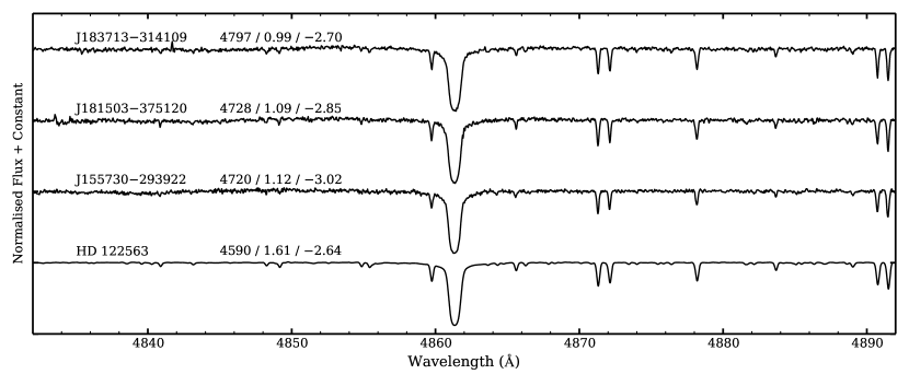
Figure 1.— Continuum-normalized Magellan/MIKE spectra for the three metal-poor stars in the bulge along with the well-studied metal-poor giant HD 122563. The spectra are centered around the H-$\beta$ line, highlighting the similarity between HD 122563 and our metal-poor stars in the bulge. We indicate the stellar parameters $T_{\mathrm{eff}}$, $\log{g}$, and $\mathrm{[Fe/H]}$ for each star, with the parameters for HD 122563 from Jofré et al. (2014).

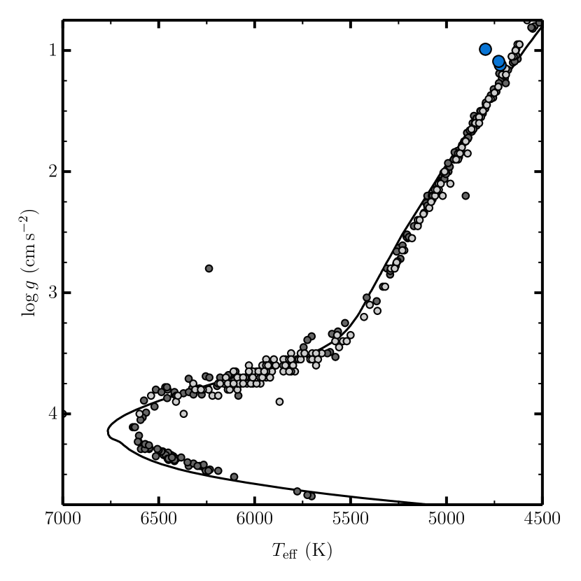
Figure 2.— Measured effective temperatures and surface gravities of metal-poor stars. We plot the locations of our three bulge metal-poor stars in blue. For comparison, we plot halo stars with $\mathrm{[Fe/H]}\lesssim-2.0$ from Yong et al. (2013a) in dark gray and from Roederer et al. (2014) in light gray. We only plot stars from Roederer et al. (2014) where the surface gravity was derived from isochrones. The solid line is a 12 Gyr, $\mathrm{[Fe/H]}=-2.5$, and [$\alpha$/Fe] $=+0.4$ Dartmouth isochrone. The Yong et al. (2013a) sample deviates from the displayed isochrone at the main sequence turn-off because Yong et al. (2013a) used the Y² isochrones (Demarque et al., 2004) to determine stellar parameters. Even though we measured our stellar parameters from excitation and ionization balance, our stars are largely in agreement with isochrone-derived surface gravities in the comparison samples.

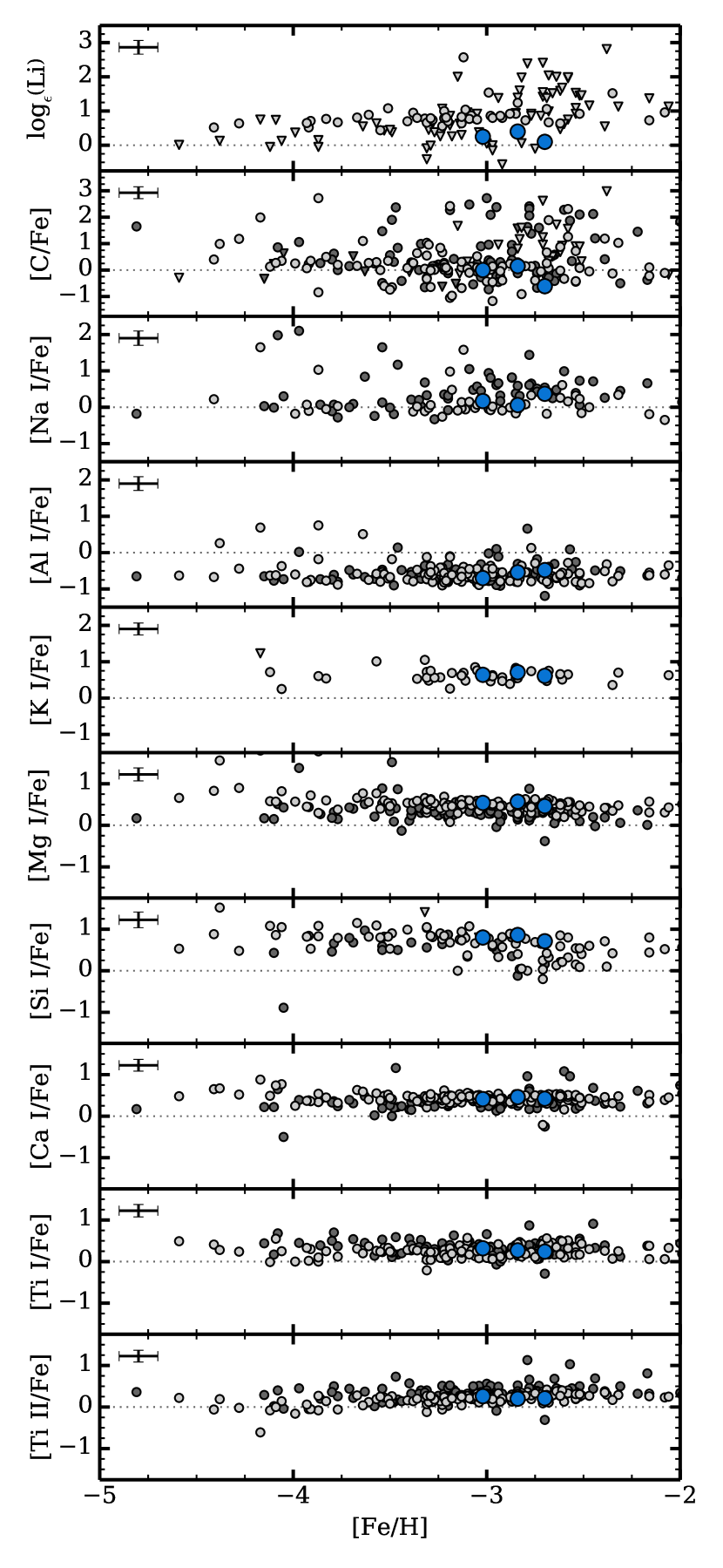
Figure 3.— Chemical abundances of Li, C, odd-Z (Na, Al, K), and $\alpha$-elements (Mg, Si, Ca, Ti) for metal-poor stars. We plot our three bulge metal-poor stars in blue, the Yong et al. (2013a) giant (i.e., $\log{g}<3$) comparison sample in dark gray, and the Roederer et al. (2014) giant sample in light gray. Measurements are indicated by circles and upper limits are shown as triangles. Typical uncertainties are given. We plot here the [K I/Fe] abundance ratios from Roederer et al. (2014) without correcting for non-LTE effects, such that they are comparable with our analysis. All other abundances from Yong et al. (2013a) and Roederer et al. (2014) shown here also assume LTE. Although the $y$-axis scale varies in each panel to accommodate the dynamic range of each abundance, the minor tick marks are spaced at $0.25$ dex in all panels.

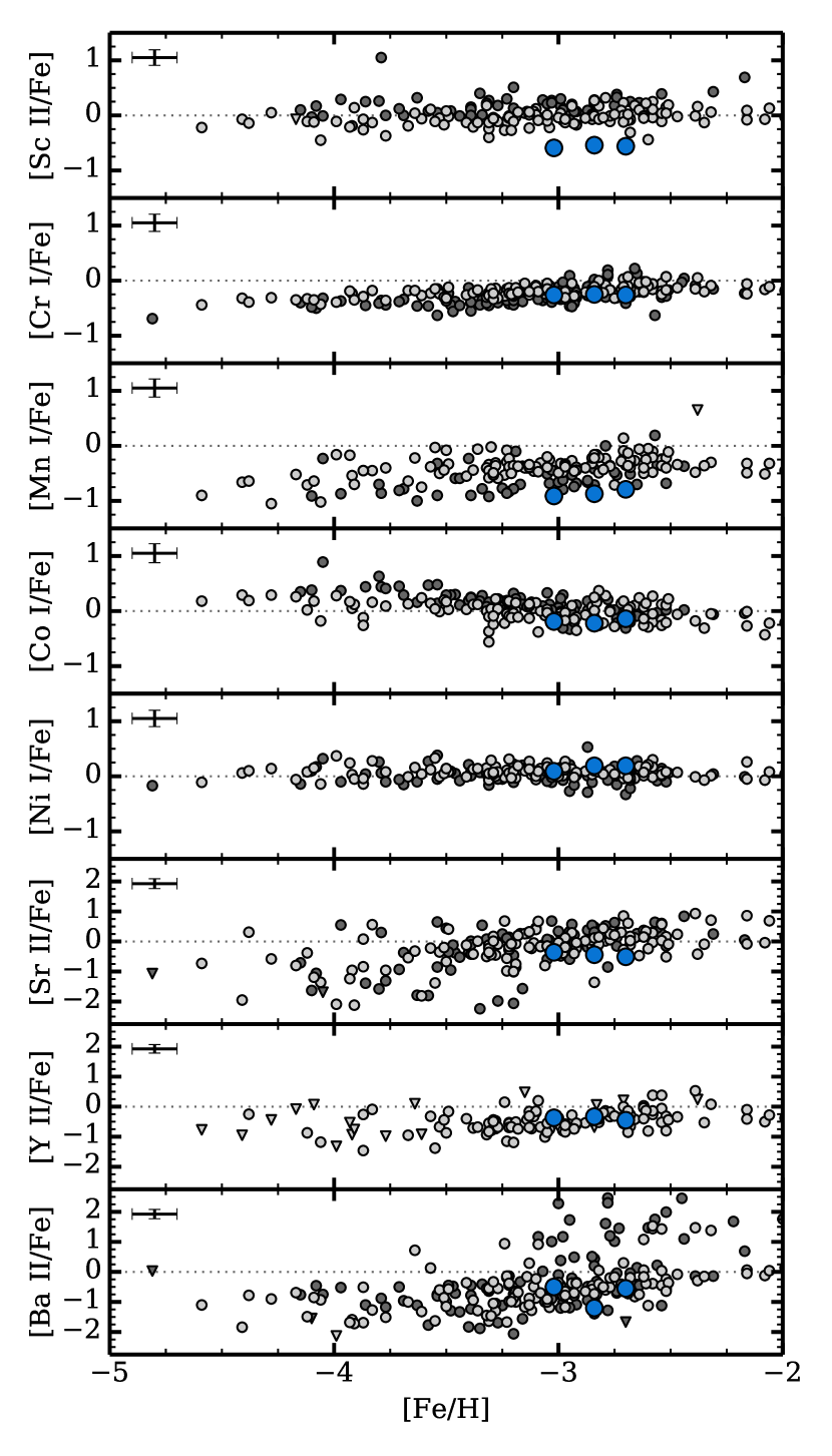
Figure 4.— Chemical abundances of Fe-peak and neutron-capture elements for metal-poor giant stars. We plot our three bulge metal-poor stars in blue, the Yong et al. (2013a) comparison sample in dark gray, and the Roederer et al. (2014) sample in light gray. Measurements are indicated with circles and upper limits are shown as triangles. Typical uncertainties are given.

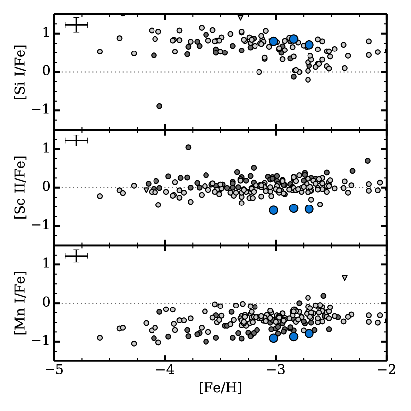
Figure 5.— Chemical abundances of Si I, Sc II, and Mn I with respect to Fe for metal-poor giant stars. We plot our three bulge metal-poor stars in blue, the Yong et al. (2013a) comparison sample in dark gray, and the Roederer et al. (2014) sample in light gray. Measurements are indicated with circles and upper limits are shown as triangles. Typical uncertainties are given. While our abundances are generally in good agreement with those measured in halo metal-poor stars, we find that silicon, scandium, and manganese are all on the extremes of the halo distribution.

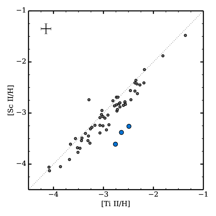
Figure 6.— Abundance ratios [Ti II/H] versus [Sc II/H]. We plot our three bulge metal-poor stars in blue and the Yong et al. (2013a) comparison sample in dark gray. Typical uncertainties are given. Our stars in the bulge significantly deviate from this relation observed in the halo.

Table 1Bulge Extremely Metal-poor Star Positions and Photometry

Object	RA	DEC	$l$	$b$	$V$	$B-V$	$J$	$H$	$K_{s}$	$W1$	$W2$
(2MASS)			(deg)	(deg)	(mag)	(mag)	(mag)	(mag)	(mag)	(mag)	(mag)
J155730.10$-$293922.7	15:57:30.1	-29:39:23	344	18	13.15	0.97	11.13	10.61	10.50	10.39	10.40
J181503.64$-$375120.7	18:15:03.6	-37:51:20	355	-10	12.87	1.01	10.80	10.29	10.19	10.12	10.13
J183713.28$-$314109.3	18:37:13.2	-31:41:09	3	-11	12.47	0.82	10.65	10.12	10.04	9.90	9.90

Table 2Bulge Extremely Metal-poor Star Kinematic Observables

Object	$v_{\rm hel}$	$\mu_{\alpha}\cos{\delta}$	$\mu_{\delta}$	$\mu_{\alpha}\cos{\delta}$	$\mu_{\delta}$
(2MASS)	(km s-1)	(mas yr-1)	(mas yr-1)	(mas yr-1)	(mas yr-1)
J155730.10$-$293922.7	$134.0\,\pm\,1.0$	$1.5\,\pm\,1.4$	$5.9\,\pm\,1.4$	$-5.68\,\pm\,2.24$	$5.26\,\pm\,2.10$
J181503.64$-$375120.7	$-77.8\,\pm\,1.0$	$-19.6\,\pm\,2.1$	$-2.9\,\pm\,2.2$	$-20.11\,\pm\,3.37$	$5.47\,\pm\,3.21$
J183713.28$-$314109.3	$-199.0\,\pm\,1.0$	$-11.4\,\pm\,1.7$	$-2.5\,\pm\,1.7$	$-8.31\,\pm\,3.18$	$-7.04\,\pm\,3.21$

Table 3Stellar Parameters of Bulge Extremely Metal-poor Stars.

Object	$T_{\rm eff}$	$\log{g}$	[Fe/H]	$\xi$
(2MASS)	(K)	(cm s-2)		(km s-1)
J155730.10$-$293922.7	4720	1.12	$-3.02$	2.88
J181503.64$-$375120.7	4728	1.09	$-2.84$	3.00
J183713.28$-$314109.3	4797	0.99	$-2.70$	2.67

Note. — We estimate the uncertainties in $T_{\mathrm{eff}}$, $\log{g}$, [Fe/H], and $\xi$ to be 100 K, 0.2 dex, 0.1 dex, and 0.1 km s^-1.

Table 4Bulge Extremely Metal-poor Star Derived Properties

Object	$d_{\odot}$	$d_{\mathrm{gc}}$	$r_{\mathrm{peri}}$	$r_{\mathrm{ap}}$	$e$	$r_{\mathrm{peri}}$	$r_{\mathrm{ap}}$	$e$
(2MASS)	(kpc)	(kpc)	(kpc)	(kpc)		(kpc)	(kpc)
J155730.10$-$293922.7	$9.8_{-2.3}^{+3.0}$	$3.4_{-1.6}^{+2.2}$	$2.9_{-2.0}^{+3.3}$	$16_{-6.8}^{+17}$	$0.747_{-0.243}^{+0.137}$	$1.7_{-1.0}^{+3.1}$	$7.3_{-3.2}^{+22}$	$0.682_{-0.269}^{+0.194}$
J181503.64$-$375120.7	$9.0_{-2.2}^{+2.8}$	$3.2_{-1.4}^{+1.5}$	$2.1_{-0.50}^{+1.9}$	$4900_{-3800}^{+3600}$	$0.999_{-0.003}^{+0.000}$	$2.1_{-0.57}^{+1.9}$	$5400_{-4200}^{+4000}$	$0.999_{-0.002}^{+0.000}$
J183713.28$-$314109.3	$9.6_{-2.3}^{+3.1}$	$3.3_{-1.5}^{+2.0}$	$1.8_{-1.1}^{+2.7}$	$88_{-72}^{+3400}$	$0.979_{-0.138}^{+0.018}$	$1.4_{-0.87}^{+2.6}$	$17_{-12}^{+210}$	$0.888_{-0.201}^{+0.093}$

Table 5Measured Equivalent Widths and Abundances of Bulge Extremely Metal-poor Stars.

				J155730$-$293922			J181503$-$375120			J183713$-$314109
Wavelength	Species	$\chi$	$\log{gf}$	EW	$\log_{\epsilon}{\rm X}$		EW	$\log_{\epsilon}{\rm X}$		EW	$\log_{\epsilon}{\rm X}$
(Å)		(eV)		(mÅ)			(mÅ)			(mÅ)
5889.95	Na I	0.00	+0.11	157.8	3.40		170.4	3.52		182.7	3.96
5895.92	Na I	0.00	$-$0.19	139.0	3.39		144.0	3.41		158.2	3.87
3829.36	Mg I	2.71	$-$0.21	156.0	5.21		169.6	5.32		$\cdots$	$\cdots$
3832.30	Mg I	2.71	+0.27	191.9	5.13		$\cdots$	$\cdots$		197.3	5.30
3838.29	Mg I	2.72	+0.49	220.0	5.13		$\cdots$	$\cdots$		229.1	5.33
3986.75	Mg I	4.35	$-$1.03	22.9	5.22		40.8	5.59		32.7	5.46
4057.51	Mg I	4.35	$-$0.89	$\cdots$	$\cdots$		34.5	5.31		39.1	5.43
4167.27	Mg I	4.35	$-$0.71	41.6	5.24		55.8	5.47		45.2	5.34
4571.10	Mg I	0.00	$-$5.69	53.0	5.09		72.4	5.36		53.8	5.24
4702.99	Mg I	4.33	$-$0.38	57.7	5.03		73.6	5.25		68.1	5.25
5172.68	Mg I	2.71	$-$0.45	180.9	5.01		198.3	5.17		194.8	5.37
5183.60	Mg I	2.72	$-$0.24	202.0	5.06		216.6	5.17		221.1	5.44
5528.40	Mg I	4.34	$-$0.50	60.3	5.10		77.7	5.33		77.4	5.42
3961.52	Al I	0.01	$-$0.34	106.5	2.73		126.6	3.07		126.6	3.27
3905.52	Si I	1.91	$-$1.09	182.2	5.30		211.0	5.53		189.9	5.52
7664.90	K I	0.00	+0.14	43.0	2.54		59.4	2.77		$\cdots$	$\cdots$
7698.96	K I	0.00	$-$0.17	38.1	2.77		56.0	3.03		43.5	2.94
4226.73	Ca I	0.00	+0.24	183.4	3.57		212.1	3.82		205.8	3.98
4283.01	Ca I	1.89	$-$0.22	47.2	3.78		59.9	3.98		63.4	4.13
4318.65	Ca I	1.89	$-$0.21	43.1	3.69		57.2	3.91		41.9	3.73
4425.44	Ca I	1.88	$-$0.36	39.0	3.73		52.6	3.95		43.6	3.87
4435.69	Ca I	1.89	$-$0.52	32.7	3.78		43.1	3.96		47.4	4.11
4454.78	Ca I	1.90	+0.26	68.5	3.62		84.5	3.86		82.8	3.97
4455.89	Ca I	1.90	$-$0.53	30.4	3.75		39.7	3.92		39.6	3.99
5262.24	Ca I	2.52	$-$0.47	$\cdots$	$\cdots$		28.2	4.27		28.8	4.34
5265.56	Ca I	2.52	$-$0.26	25.2	4.00		37.6	4.24		38.9	4.32
5349.47	Ca I	2.71	$-$0.31	11.4	3.85		17.1	4.06		17.9	4.13
5581.97	Ca I	2.52	$-$0.56	$\cdots$	$\cdots$		$\cdots$	$\cdots$		21.5	4.24
5588.76	Ca I	2.52	+0.21	34.6	3.69		45.7	3.87		52.3	4.05
5590.12	Ca I	2.52	$-$0.57	$\cdots$	$\cdots$		18.2	4.11		16.9	4.12
5594.47	Ca I	2.52	+0.10	27.0	3.65		40.4	3.89		41.9	3.99
5598.49	Ca I	2.52	$-$0.09	$\cdots$	$\cdots$		31.4	3.93		34.7	4.05
5601.28	Ca I	2.53	$-$0.52	$\cdots$	$\cdots$		14.4	3.95		$\cdots$	$\cdots$
5857.45	Ca I	2.93	+0.23	16.2	3.71		23.7	3.92		25.8	4.01
6102.72	Ca I	1.88	$-$0.79	24.2	3.69		38.3	3.95		43.7	4.12
6122.22	Ca I	1.89	$-$0.32	58.6	3.80		67.2	3.91		73.5	4.11
6162.17	Ca I	1.90	$-$0.09	68.4	3.72		75.6	3.81		79.5	3.98
6169.06	Ca I	2.52	$-$0.80	5.2	3.70		12.7	4.13		12.0	4.15
6169.56	Ca I	2.53	$-$0.48	11.9	3.78		17.0	3.96		18.8	4.07
6439.07	Ca I	2.52	+0.47	45.1	3.55		58.0	3.73		59.5	3.84
6449.81	Ca I	2.52	$-$0.50	$\cdots$	$\cdots$		20.4	4.05		17.2	4.02
4246.82	Sc II	0.32	+0.24	$\cdots$	$-$0.70		$\cdots$	$-$0.50		$\cdots$	$-$0.15
4314.08	Sc II	0.62	$-$0.10	$\cdots$	$-$0.50		$\cdots$	$-$0.10		$\cdots$	0.00
4325.00	Sc II	0.59	$-$0.44	$\cdots$	$-$0.40		$\cdots$	$-$0.10		$\cdots$	0.00
4400.39	Sc II	0.61	$-$0.54	$\cdots$	$-$0.40		$\cdots$	$-$0.30		$\cdots$	$-$0.15
4415.54	Sc II	0.59	$-$0.67	$\cdots$	$-$0.25		$\cdots$	$-$0.25		$\cdots$	$-$0.15
5031.01	Sc II	1.36	$-$0.40	$\cdots$	$\cdots$		$\cdots$	$\cdots$		$\cdots$	$-$0.35
5526.78	Sc II	1.77	+0.02	$\cdots$	$-$0.50		$\cdots$	$-$0.30		$\cdots$	$-$0.10
5657.91	Sc II	1.51	$-$0.60	$\cdots$	$\cdots$		$\cdots$	$-$0.05		$\cdots$	0.00
3904.78	Ti I	0.90	+0.03	20.7	2.45		$\cdots$	$\cdots$		$\cdots$	$\cdots$
3989.76	Ti I	0.02	$-$0.06	57.3	2.16		65.9	2.30		67.7	2.48
3998.64	Ti I	0.05	+0.01	59.7	2.18		63.9	2.23		69.6	2.48
4008.93	Ti I	0.02	$-$1.02	21.8	2.44		20.5	2.41		22.2	2.55
4512.73	Ti I	0.84	$-$0.42	$\cdots$	$\cdots$		11.6	2.39		12.0	2.49
4518.02	Ti I	0.83	$-$0.27	9.4	2.11		21.1	2.53		$\cdots$	$\cdots$
4533.25	Ti I	0.85	+0.53	38.6	2.09		47.2	2.23		49.2	2.38
4534.78	Ti I	0.84	+0.34	32.8	2.17		38.3	2.27		43.3	2.45
4535.57	Ti I	0.83	+0.12	22.0	2.15		32.8	2.38		32.4	2.47
4544.69	Ti I	0.82	$-$0.52	$\cdots$	$\cdots$		$\cdots$	$\cdots$		12.9	2.60
4548.76	Ti I	0.83	$-$0.30	12.5	2.28		16.5	2.42		17.2	2.53
4555.49	Ti I	0.85	$-$0.43	$\cdots$	$\cdots$		$\cdots$	$\cdots$		12.1	2.51
4656.47	Ti I	0.00	$-$1.29	11.7	2.22		18.5	2.45		16.6	2.50
4681.91	Ti I	0.05	$-$1.01	20.9	2.28		27.9	2.45		23.2	2.46
4840.87	Ti I	0.90	$-$0.45	11.6	2.43		8.8	2.31		11.2	2.51
4981.73	Ti I	0.84	+0.56	39.4	1.99		60.1	2.30		57.1	2.38
4991.07	Ti I	0.84	+0.44	44.1	2.18		51.4	2.29		53.4	2.44
4999.50	Ti I	0.83	+0.31	33.7	2.12		46.8	2.34		48.6	2.48
5007.21	Ti I	0.82	+0.17	38.6	2.33		48.7	2.49		59.6	2.78
5014.28	Ti I	0.81	+0.11	$\cdots$	$\cdots$		$\cdots$	$\cdots$		43.5	2.57
5016.16	Ti I	0.85	$-$0.52	16.1	2.58		$\cdots$	$\cdots$		$\cdots$	$\cdots$
5020.02	Ti I	0.84	$-$0.36	10.5	2.20		19.3	2.51		23.5	2.70
5024.84	Ti I	0.82	$-$0.55	16.7	2.59		$\cdots$	$\cdots$		$\cdots$	$\cdots$
5036.46	Ti I	1.44	+0.19	$\cdots$	$\cdots$		17.3	2.62		7.5	2.29
5039.96	Ti I	0.02	$-$1.13	17.8	2.23		21.7	2.34		24.6	2.52
5064.65	Ti I	0.05	$-$0.94	26.2	2.28		36.3	2.47		40.4	2.66
5173.74	Ti I	0.00	$-$1.06	19.7	2.17		29.9	2.41		20.7	2.32
5192.97	Ti I	0.02	$-$0.95	28.3	2.28		29.5	2.31		24.6	2.32
5210.39	Ti I	0.05	$-$0.83	25.5	2.14		36.4	2.35		30.3	2.36
3759.29	Ti II	0.61	+0.28	183.9	2.30		$\cdots$	$\cdots$		$\cdots$	$\cdots$
3761.32	Ti II	0.57	+0.18	185.0	2.36		$\cdots$	$\cdots$		$\cdots$	$\cdots$
3813.39	Ti II	0.61	$-$2.02	89.4	2.74		89.7	2.67		93.1	2.84
3882.29	Ti II	1.12	$-$1.71	44.6	2.16		61.3	2.42		61.9	2.47
3913.46	Ti II	1.12	$-$0.42	109.5	2.13		130.9	2.46		$\cdots$	$\cdots$
4012.40	Ti II	0.57	$-$1.75	96.3	2.40		91.7	2.24		111.4	2.76
4025.12	Ti II	0.61	$-$1.98	70.7	2.18		82.2	2.34		84.8	2.48
4028.34	Ti II	1.89	$-$0.96	41.9	2.24		46.7	2.30		55.6	2.46
4053.83	Ti II	1.89	$-$1.21	31.1	2.27		36.6	2.36		41.4	2.46
4161.53	Ti II	1.08	$-$2.16	34.7	2.28		40.3	2.36		51.6	2.58
4163.63	Ti II	2.59	$-$0.40	32.2	2.29		39.7	2.41		47.9	2.56
4184.31	Ti II	1.08	$-$2.51	22.0	2.36		29.7	2.52		33.0	2.60
4290.22	Ti II	1.16	$-$0.93	93.2	2.09		111.7	2.35		$\cdots$	$\cdots$
4300.05	Ti II	1.18	$-$0.49	106.6	1.92		122.0	2.12		124.2	2.33
4330.72	Ti II	1.18	$-$2.06	30.6	2.18		38.8	2.32		45.3	2.45
4337.91	Ti II	1.08	$-$0.96	98.6	2.09		100.6	2.07		112.6	2.41
4394.06	Ti II	1.22	$-$1.78	48.0	2.23		52.6	2.29		60.7	2.45
4395.03	Ti II	1.08	$-$0.54	115.4	1.96		127.3	2.10		131.5	2.34
4395.84	Ti II	1.24	$-$1.93	34.3	2.18		44.3	2.33		50.9	2.46
4398.29	Ti II	1.21	$-$2.65	8.6	2.14		$\cdots$	$\cdots$		15.0	2.41
4399.77	Ti II	1.24	$-$1.19	76.5	2.11		86.0	2.21		93.2	2.44
4409.52	Ti II	1.23	$-$2.37	19.6	2.29		17.0	2.21		22.3	2.36
4417.71	Ti II	1.17	$-$1.19	80.0	2.07		89.7	2.19		93.6	2.35
4418.33	Ti II	1.24	$-$1.97	31.8	2.17		41.1	2.31		45.0	2.40
4441.73	Ti II	1.18	$-$2.41	21.6	2.31		31.2	2.51		37.4	2.64
4443.80	Ti II	1.08	$-$0.72	104.4	1.91		111.9	1.97		122.1	2.32
4444.55	Ti II	1.12	$-$2.24	27.6	2.20		36.2	2.35		48.3	2.57
4450.48	Ti II	1.08	$-$1.52	72.1	2.15		80.9	2.25		90.7	2.51
4464.45	Ti II	1.16	$-$1.81	50.5	2.21		55.5	2.27		64.2	2.43
4468.52	Ti II	1.13	$-$0.60	108.9	1.92		117.7	2.00		128.4	2.36
4470.85	Ti II	1.17	$-$2.02	33.5	2.15		39.6	2.24		49.3	2.43
4488.34	Ti II	3.12	$-$0.82	$\cdots$	$\cdots$		$\cdots$	$\cdots$		11.3	2.68
4493.52	Ti II	1.08	$-$3.02	12.1	2.50		20.0	2.75		18.7	2.72
4501.27	Ti II	1.12	$-$0.77	105.1	2.00		106.3	1.94		117.3	2.29
4529.48	Ti II	1.57	$-$2.03	32.2	2.61		32.5	2.61		43.4	2.81
4533.96	Ti II	1.24	$-$0.53	109.3	1.97		109.5	1.91		125.9	2.35
4545.14	Ti II	1.13	$-$1.81	18.9	1.56		$\cdots$	$\cdots$		26.6	1.75
4563.77	Ti II	1.22	$-$0.96	97.6	2.16		101.9	2.17		113.7	2.50
4571.97	Ti II	1.57	$-$0.32	92.8	1.86		100.8	1.94		114.6	2.30
4583.41	Ti II	1.16	$-$2.92	$\cdots$	$\cdots$		13.3	2.52		16.2	2.63
4589.91	Ti II	1.24	$-$1.79	54.5	2.32		63.8	2.43		70.7	2.58
4636.32	Ti II	1.16	$-$3.02	$\cdots$	$\cdots$		9.6	2.46		$\cdots$	$\cdots$
4657.20	Ti II	1.24	$-$2.24	20.7	2.15		29.8	2.34		33.0	2.42
4708.66	Ti II	1.24	$-$2.34	22.2	2.28		26.6	2.37		32.7	2.51
4779.98	Ti II	2.05	$-$1.37	20.2	2.23		28.9	2.42		34.1	2.52
4798.53	Ti II	1.08	$-$2.68	18.5	2.32		22.5	2.41		30.6	2.60
4805.09	Ti II	2.06	$-$1.10	35.8	2.29		41.5	2.37		51.7	2.55
4865.61	Ti II	1.12	$-$2.81	15.9	2.41		19.6	2.51		17.9	2.48
4911.18	Ti II	3.12	$-$0.34	$\cdots$	$\cdots$		$\cdots$	$\cdots$		13.2	2.22
5129.16	Ti II	1.89	$-$1.24	27.4	2.03		43.9	2.30		47.5	2.37
5185.90	Ti II	1.89	$-$1.49	26.8	2.26		34.0	2.38		35.3	2.42
5188.69	Ti II	1.58	$-$1.05	72.7	2.14		83.3	2.26		83.5	2.33
5226.54	Ti II	1.57	$-$1.26	55.6	2.10		66.0	2.22		67.2	2.29
5336.79	Ti II	1.58	$-$1.59	41.7	2.22		46.7	2.29		52.1	2.39
5381.02	Ti II	1.57	$-$1.92	20.3	2.13		35.5	2.43		38.0	2.49
5418.77	Ti II	1.58	$-$2.00	19.6	2.20		18.8	2.17		29.4	2.42
4379.24	V I	2.10	$-$2.71	$\cdots$	0.46		$\cdots$	0.58		$\cdots$	0.68
3916.41	V II	1.43	$-$1.05	19.0	1.21		24.5	1.34		25.3	1.36
3951.96	V II	1.48	$-$0.78	28.4	1.22		38.3	1.39		31.8	1.28
4005.71	V II	1.82	$-$0.52	$\cdots$	$\cdots$		32.5	1.42		35.0	1.47
4023.38	V II	1.80	$-$0.69	17.2	1.21		22.4	1.34		27.7	1.46
4035.62	V II	1.79	$-$0.77	$\cdots$	$\cdots$		41.5	1.78		$\cdots$	$\cdots$
3908.76	Cr I	1.00	$-$1.00	$\cdots$	$\cdots$		$\cdots$	$\cdots$		19.6	2.83
4254.33	Cr I	0.00	$-$0.11	98.1	2.04		99.1	1.99		107.7	2.41
4274.80	Cr I	0.00	$-$0.22	93.6	2.05		101.2	2.13		109.9	2.56
4289.72	Cr I	0.00	$-$0.37	85.6	2.03		99.7	2.25		107.8	2.66
4337.57	Cr I	0.97	$-$1.11	$\cdots$	$\cdots$		24.9	2.85		$\cdots$	$\cdots$
4545.95	Cr I	0.94	$-$1.37	$\cdots$	$\cdots$		$\cdots$	$\cdots$		11.4	2.72
4580.06	Cr I	0.94	$-$1.65	$\cdots$	$\cdots$		15.7	3.06		$\cdots$	$\cdots$
4600.75	Cr I	1.00	$-$1.26	$\cdots$	$\cdots$		11.1	2.57		$\cdots$	$\cdots$
4616.14	Cr I	0.98	$-$1.19	15.9	2.64		13.5	2.57		14.5	2.69
4626.19	Cr I	0.97	$-$1.32	$\cdots$	$\cdots$		17.2	2.81		$\cdots$	$\cdots$
4646.15	Cr I	1.03	$-$0.74	23.0	2.44		29.2	2.58		33.4	2.75
4651.28	Cr I	0.98	$-$1.46	$\cdots$	$\cdots$		8.7	2.62		6.3	2.56
4652.16	Cr I	1.00	$-$1.03	16.0	2.50		18.3	2.58		23.3	2.80
5206.04	Cr I	0.94	+0.02	67.9	2.24		80.4	2.40		85.1	2.65
5208.42	Cr I	0.94	+0.16	90.4	2.45		96.9	2.52		$\cdots$	$\cdots$
5247.56	Cr I	0.96	$-$1.64	$\cdots$	$\cdots$		$\cdots$	$\cdots$		8.4	2.78
5296.69	Cr I	0.98	$-$1.36	8.6	2.43		11.0	2.56		12.6	2.71
5298.28	Cr I	0.98	$-$1.14	$\cdots$	$\cdots$		22.5	2.69		24.2	2.82
5345.80	Cr I	1.00	$-$0.95	16.3	2.35		31.4	2.70		24.7	2.67
5348.31	Cr I	1.00	$-$1.21	22.5	2.77		12.0	2.46		12.6	2.58
5409.77	Cr I	1.03	$-$0.67	25.0	2.32		34.3	2.50		40.0	2.70
4558.59	Cr II	4.07	$-$0.66	10.7	2.74		16.3	2.94		24.4	3.12
4588.14	Cr II	4.07	$-$0.83	9.2	2.83		14.0	3.02		17.2	3.09
4030.75	Mn I	0.00	$-$0.48	$\cdots$	1.51		$\cdots$	1.68		$\cdots$	1.93
4033.06	Mn I	0.00	$-$0.62	$\cdots$	1.36		$\cdots$	1.63		$\cdots$	1.88
4034.48	Mn I	0.00	$-$0.81	$\cdots$	1.46		$\cdots$	1.63		$\cdots$	1.78
4041.36	Mn I	2.11	+0.28	$\cdots$	1.66		$\cdots$	1.88		$\cdots$	2.18
3689.46	Fe I	2.94	$-$0.17	$\cdots$	$\cdots$		57.6	4.60		54.1	4.62
3753.61	Fe I	2.18	$-$0.89	58.9	4.43		60.9	4.42		65.6	4.65
3765.54	Fe I	3.24	+0.48	65.7	4.49		70.7	4.54		75.7	4.79
3786.68	Fe I	1.01	$-$2.19	$\cdots$	$\cdots$		82.9	4.74		82.5	4.91
3805.34	Fe I	3.30	+0.31	58.2	4.53		61.4	4.56		63.4	4.70
3839.26	Fe I	3.05	$-$0.33	50.8	4.68		55.3	4.74		42.9	4.58
3845.17	Fe I	2.42	$-$1.39	28.0	4.51		$\cdots$	$\cdots$		33.8	4.71
3846.80	Fe I	3.25	$-$0.02	40.9	4.40		60.5	4.77		46.4	4.57
3850.82	Fe I	0.99	$-$1.75	$\cdots$	$\cdots$		104.6	4.71		$\cdots$	$\cdots$
3852.57	Fe I	2.18	$-$1.18	56.3	4.59		63.9	4.70		65.8	4.88
3863.74	Fe I	2.69	$-$1.43	19.6	4.66		28.2	4.87		34.5	5.08
3867.22	Fe I	3.02	$-$0.45	27.8	4.28		43.8	4.60		55.5	4.91
3885.51	Fe I	2.42	$-$1.09	41.6	4.48		38.9	4.42		42.1	4.56
3887.05	Fe I	0.91	$-$1.14	110.7	4.20		$\cdots$	$\cdots$		$\cdots$	$\cdots$
3902.95	Fe I	1.56	$-$0.44	117.4	4.45		119.5	4.38		$\cdots$	$\cdots$
3917.18	Fe I	0.99	$-$2.15	79.3	4.55		93.6	4.79		96.5	5.07
3940.88	Fe I	0.96	$-$2.60	49.8	4.35		69.8	4.69		67.6	4.81
3949.95	Fe I	2.18	$-$1.25	59.3	4.66		69.9	4.83		61.6	4.79
3977.74	Fe I	2.20	$-$1.12	66.1	4.67		67.4	4.66		63.8	4.72
4001.66	Fe I	2.18	$-$1.90	21.5	4.53		31.9	4.76		27.2	4.74
4005.24	Fe I	1.56	$-$0.58	112.8	4.37		118.9	4.40		$\cdots$	$\cdots$
4007.27	Fe I	2.76	$-$1.28	19.5	4.54		26.5	4.71		27.3	4.80
4014.53	Fe I	3.05	$-$0.59	$\cdots$	$\cdots$		$\cdots$	$\cdots$		64.4	5.20
4021.87	Fe I	2.76	$-$0.73	39.7	4.43		47.1	4.56		55.2	4.80
4032.63	Fe I	1.49	$-$2.38	26.9	4.30		48.8	4.70		49.4	4.83
4044.61	Fe I	2.83	$-$1.22	18.2	4.52		26.3	4.72		28.3	4.84
4058.22	Fe I	3.21	$-$1.11	$\cdots$	$\cdots$		19.4	4.89		16.6	4.86
4062.44	Fe I	2.85	$-$0.86	34.3	4.55		37.3	4.60		42.1	4.77
4067.27	Fe I	2.56	$-$1.42	24.2	4.55		38.9	4.84		36.0	4.87
4067.98	Fe I	3.21	$-$0.47	28.5	4.47		38.1	4.65		36.5	4.69
4070.77	Fe I	3.24	$-$0.79	14.8	4.45		18.6	4.58		23.8	4.77
4073.76	Fe I	3.27	$-$0.90	$\cdots$	$\cdots$		21.2	4.79		26.7	4.98
4076.63	Fe I	3.21	$-$0.37	41.4	4.62		52.9	4.81		52.5	4.90
4079.84	Fe I	2.86	$-$1.36	10.7	4.41		19.3	4.72		21.0	4.83
4095.97	Fe I	2.59	$-$1.48	16.0	4.41		25.2	4.66		29.9	4.84
4098.18	Fe I	3.24	$-$0.88	18.8	4.66		23.5	4.79		23.4	4.84
4109.80	Fe I	2.85	$-$0.94	29.7	4.52		42.1	4.76		34.0	4.68
4114.44	Fe I	2.83	$-$1.30	13.0	4.40		24.0	4.73		22.3	4.76
4120.21	Fe I	2.99	$-$1.27	19.8	4.78		22.1	4.84		27.2	5.03
4121.80	Fe I	2.83	$-$1.45	$\cdots$	$\cdots$		28.6	4.98		24.3	4.95
4132.06	Fe I	1.61	$-$0.68	115.3	4.48		119.8	4.47		$\cdots$	$\cdots$
4132.90	Fe I	2.85	$-$1.01	28.8	4.56		41.4	4.80		40.5	4.87
4134.68	Fe I	2.83	$-$0.65	39.9	4.40		56.2	4.68		54.4	4.74
4137.00	Fe I	3.42	$-$0.45	17.9	4.41		22.2	4.52		26.1	4.68
4139.93	Fe I	0.99	$-$3.63	12.1	4.49		25.8	4.89		18.5	4.81
4143.41	Fe I	3.05	$-$0.20	52.6	4.44		$\cdots$	$\cdots$		65.5	4.77
4143.87	Fe I	1.56	$-$0.51	117.4	4.28		120.4	4.25		130.5	4.72
4147.67	Fe I	1.48	$-$2.07	55.9	4.47		65.6	4.62		70.7	4.86
4152.17	Fe I	0.96	$-$3.23	34.6	4.62		48.1	4.86		45.5	4.94
4153.90	Fe I	3.40	$-$0.32	29.4	4.53		37.4	4.69		41.5	4.84
4154.50	Fe I	2.83	$-$0.69	43.5	4.50		50.8	4.62		49.1	4.68
4154.81	Fe I	3.37	$-$0.40	25.9	4.50		38.0	4.74		31.7	4.69
4156.80	Fe I	2.83	$-$0.81	43.6	4.62		45.4	4.64		47.7	4.77
4157.78	Fe I	3.42	$-$0.40	20.2	4.42		33.2	4.71		35.7	4.83
4158.79	Fe I	3.43	$-$0.67	12.4	4.44		16.1	4.58		18.7	4.71
4174.91	Fe I	0.91	$-$2.94	55.1	4.63		68.5	4.83		58.9	4.81
4175.64	Fe I	2.85	$-$0.83	32.1	4.44		48.8	4.74		43.9	4.74
4181.76	Fe I	2.83	$-$0.37	54.6	4.37		65.4	4.53		70.9	4.77
4182.38	Fe I	3.02	$-$1.18	12.1	4.45		16.0	4.60		20.2	4.79
4184.89	Fe I	2.83	$-$0.87	34.0	4.49		39.7	4.60		36.7	4.62
4187.04	Fe I	2.45	$-$0.51	75.2	4.43		82.7	4.52		83.6	4.71
4187.80	Fe I	2.42	$-$0.51	74.4	4.37		87.1	4.57		86.7	4.74
4191.43	Fe I	2.47	$-$0.67	65.9	4.43		72.9	4.53		77.8	4.76
4195.33	Fe I	3.33	$-$0.49	27.9	4.58		41.0	4.83		33.5	4.76
4196.21	Fe I	3.40	$-$0.70	18.4	4.63		$\cdots$	$\cdots$		18.8	4.71
4199.10	Fe I	3.05	+0.16	62.3	4.23		74.4	4.43		74.9	4.57
4202.03	Fe I	1.49	$-$0.69	113.6	4.25		121.7	4.33		124.3	4.64
4216.18	Fe I	0.00	$-$3.36	96.9	4.69		99.8	4.68		97.5	4.87
4217.55	Fe I	3.43	$-$0.48	24.7	4.61		30.6	4.73		28.9	4.76
4222.21	Fe I	2.45	$-$0.91	47.3	4.31		61.6	4.53		64.9	4.72
4227.43	Fe I	3.33	+0.27	66.7	4.54		82.8	4.80		91.2	5.13
4233.60	Fe I	2.48	$-$0.58	67.2	4.36		74.6	4.46		78.8	4.69
4238.81	Fe I	3.40	$-$0.23	30.7	4.45		41.7	4.65		41.9	4.73
4247.43	Fe I	3.37	$-$0.24	39.5	4.59		56.0	4.87		56.5	4.97
4250.12	Fe I	2.47	$-$0.38	77.0	4.32		86.9	4.47		88.4	4.68
4250.79	Fe I	1.56	$-$0.71	105.9	4.15		116.9	4.29		121.0	4.64
4260.47	Fe I	2.40	+0.08	105.8	4.37		108.1	4.33		120.0	4.81
4271.15	Fe I	2.45	$-$0.34	$\cdots$	$\cdots$		103.0	4.71		99.1	4.83
4282.40	Fe I	2.18	$-$0.78	72.3	4.27		81.0	4.40		88.0	4.71
4337.05	Fe I	1.56	$-$1.70	80.0	4.56		85.1	4.60		86.2	4.82
4352.73	Fe I	2.22	$-$1.29	58.7	4.57		70.7	4.74		62.8	4.74
4375.93	Fe I	0.00	$-$3.00	110.3	4.51		$\cdots$	$\cdots$		116.3	4.83
4388.41	Fe I	3.60	$-$0.68	$\cdots$	$\cdots$		12.3	4.61		19.6	4.90
4404.75	Fe I	1.56	$-$0.15	136.4	4.13		$\cdots$	$\cdots$		$\cdots$	$\cdots$
4407.71	Fe I	2.18	$-$1.97	34.7	4.77		45.7	4.96		45.4	5.06
4415.12	Fe I	1.61	$-$0.62	112.2	4.15		121.3	4.25		123.2	4.55
4422.57	Fe I	2.85	$-$1.11	31.0	4.64		34.4	4.70		41.8	4.92
4427.31	Fe I	0.05	$-$2.92	102.2	4.30		118.9	4.57		115.4	4.76
4430.61	Fe I	2.22	$-$1.66	28.7	4.39		46.1	4.70		45.7	4.80
4442.34	Fe I	2.20	$-$1.23	54.1	4.38		67.0	4.57		70.3	4.76
4443.19	Fe I	2.86	$-$1.04	21.4	4.36		33.1	4.62		35.3	4.74
4447.72	Fe I	2.22	$-$1.34	45.2	4.37		65.4	4.67		57.1	4.67
4454.38	Fe I	2.83	$-$1.30	15.4	4.42		19.9	4.55		$\cdots$	$\cdots$
4459.12	Fe I	2.18	$-$1.28	63.3	4.55		82.2	4.85		81.3	4.99
4461.65	Fe I	0.09	$-$3.19	95.0	4.47		105.6	4.60		100.9	4.75
4466.55	Fe I	2.83	$-$0.60	60.6	4.61		69.2	4.73		70.9	4.88
4476.02	Fe I	2.85	$-$0.82	49.6	4.67		55.6	4.75		62.1	4.97
4484.22	Fe I	3.60	$-$0.86	10.0	4.67		10.0	4.67		20.5	5.09
4489.74	Fe I	0.12	$-$3.90	60.0	4.60		73.8	4.79		$\cdots$	$\cdots$
4494.56	Fe I	2.20	$-$1.14	60.0	4.37		78.8	4.65		79.6	4.83
4528.61	Fe I	2.18	$-$0.82	77.5	4.32		$\cdots$	$\cdots$		96.9	4.82
4531.15	Fe I	1.48	$-$2.10	58.7	4.43		70.0	4.59		68.5	4.71
4592.65	Fe I	1.56	$-$2.46	43.4	4.63		53.9	4.79		55.8	4.94
4602.94	Fe I	1.49	$-$2.21	58.7	4.53		67.7	4.65		65.9	4.77
4630.12	Fe I	2.28	$-$2.59	$\cdots$	$\cdots$		10.4	4.84		13.2	5.03
4632.91	Fe I	1.61	$-$2.91	18.1	4.62		19.9	4.67		21.4	4.81
4647.43	Fe I	2.95	$-$1.35	14.8	4.55		19.3	4.70		18.8	4.76
4678.85	Fe I	3.60	$-$0.83	$\cdots$	$\cdots$		16.3	4.85		19.1	5.00
4691.41	Fe I	2.99	$-$1.52	$\cdots$	$\cdots$		18.1	4.87		20.0	5.00
4707.27	Fe I	3.24	$-$1.08	16.0	4.66		25.1	4.90		23.7	4.94
4710.28	Fe I	3.02	$-$1.61	9.4	4.67		19.0	5.02		14.7	4.96
4733.59	Fe I	1.49	$-$2.99	20.1	4.59		28.4	4.78		27.5	4.87
4736.77	Fe I	3.21	$-$0.75	23.5	4.49		35.0	4.72		39.8	4.89
4786.81	Fe I	3.00	$-$1.61	$\cdots$	$\cdots$		$\cdots$	$\cdots$		13.7	4.89
4789.65	Fe I	3.53	$-$0.96	$\cdots$	$\cdots$		$\cdots$	$\cdots$		9.8	4.70
4859.74	Fe I	2.88	$-$0.76	52.2	4.61		56.6	4.67		62.1	4.87
4871.32	Fe I	2.87	$-$0.36	59.1	4.30		69.5	4.44		70.8	4.59
4872.14	Fe I	2.88	$-$0.57	47.3	4.34		57.7	4.49		66.2	4.74
4890.76	Fe I	2.88	$-$0.39	54.9	4.28		66.3	4.44		72.7	4.67
4891.49	Fe I	2.85	$-$0.11	72.1	4.23		81.1	4.35		85.7	4.58
4903.31	Fe I	2.88	$-$0.93	29.6	4.39		34.8	4.49		44.9	4.75
4918.99	Fe I	2.85	$-$0.34	63.5	4.32		$\cdots$	$\cdots$		71.3	4.54
4920.50	Fe I	2.83	+0.07	85.2	4.23		92.3	4.31		96.3	4.56
4924.77	Fe I	2.28	$-$2.11	$\cdots$	$\cdots$		23.5	4.72		19.4	4.71
4938.81	Fe I	2.88	$-$1.08	26.8	4.48		36.8	4.67		35.9	4.73
4939.69	Fe I	0.86	$-$3.25	40.9	4.46		52.7	4.65		49.5	4.73
4946.39	Fe I	3.37	$-$1.17	$\cdots$	$\cdots$		15.8	4.87		14.5	4.89
4966.09	Fe I	3.33	$-$0.87	17.1	4.55		31.5	4.89		25.8	4.85
4973.10	Fe I	3.96	$-$0.95	$\cdots$	$\cdots$		12.8	5.24		$\cdots$	$\cdots$
4994.13	Fe I	0.92	$-$2.97	62.0	4.57		62.8	4.57		55.3	4.60
5001.87	Fe I	3.88	+0.05	22.8	4.43		22.0	4.42		23.3	4.51
5006.12	Fe I	2.83	$-$0.61	48.6	4.32		58.1	4.46		$\cdots$	$\cdots$
5012.07	Fe I	0.86	$-$2.64	75.6	4.36		97.2	4.67		94.4	4.84
5022.24	Fe I	3.98	$-$0.53	$\cdots$	$\cdots$		$\cdots$	$\cdots$		8.7	4.70
5041.07	Fe I	0.96	$-$3.09	62.8	4.74		71.1	4.85		67.8	4.96
5041.76	Fe I	1.49	$-$2.20	63.4	4.51		81.3	4.75		83.4	4.96
5049.82	Fe I	2.28	$-$1.35	45.9	4.35		66.2	4.65		48.8	4.50
5051.63	Fe I	0.92	$-$2.76	73.8	4.52		88.4	4.71		76.3	4.71
5060.08	Fe I	0.00	$-$5.46	$\cdots$	$\cdots$		17.4	5.14		$\cdots$	$\cdots$
5068.77	Fe I	2.94	$-$1.04	26.4	4.48		30.2	4.56		30.4	4.65
5074.75	Fe I	4.22	$-$0.20	$\cdots$	$\cdots$		19.4	4.99		16.5	4.96
5079.22	Fe I	2.20	$-$2.10	23.4	4.59		27.4	4.68		31.3	4.85
5079.74	Fe I	0.99	$-$3.25	33.3	4.47		56.6	4.84		50.2	4.88
5083.34	Fe I	0.96	$-$2.84	55.6	4.38		68.7	4.56		68.7	4.71
5090.77	Fe I	4.26	$-$0.36	$\cdots$	$\cdots$		$\cdots$	$\cdots$		9.6	4.90
5098.70	Fe I	2.18	$-$2.03	37.1	4.76		$\cdots$	$\cdots$		39.8	4.91
5110.41	Fe I	0.00	$-$3.76	87.0	4.57		95.0	4.67		95.9	4.91
5123.72	Fe I	1.01	$-$3.06	57.9	4.68		63.5	4.76		64.3	4.92
5125.12	Fe I	4.22	$-$0.14	$\cdots$	$\cdots$		13.7	4.75		22.0	5.05
5127.36	Fe I	0.92	$-$3.25	48.4	4.62		58.1	4.76		54.2	4.85
5131.47	Fe I	2.22	$-$2.52	9.7	4.58		11.1	4.66		26.3	5.19
5133.69	Fe I	4.18	+0.14	$\cdots$	$\cdots$		30.1	4.84		33.1	4.96
5137.38	Fe I	4.18	$-$0.40	$\cdots$	$\cdots$		9.1	4.77		12.8	4.98
5141.74	Fe I	2.42	$-$2.24	13.2	4.69		$\cdots$	$\cdots$		18.0	4.94
5142.93	Fe I	0.96	$-$3.08	54.0	4.59		65.1	4.74		62.5	4.85
5150.84	Fe I	0.99	$-$3.04	41.2	4.39		55.7	4.60		55.4	4.74
5151.91	Fe I	1.01	$-$3.32	28.4	4.47		$\cdots$	$\cdots$		41.8	4.83
5162.27	Fe I	4.18	+0.02	20.8	4.75		27.9	4.91		25.9	4.93
5166.28	Fe I	0.00	$-$4.12	60.0	4.53		69.0	4.65		71.8	4.86
5171.60	Fe I	1.49	$-$1.72	$\cdots$	$\cdots$		99.7	4.53		94.7	4.65
5191.45	Fe I	3.04	$-$0.55	38.3	4.32		48.5	4.48		53.5	4.66
5192.34	Fe I	3.00	$-$0.42	51.8	4.36		53.3	4.38		61.2	4.61
5194.94	Fe I	1.56	$-$2.02	68.1	4.45		78.6	4.59		73.1	4.66
5198.71	Fe I	2.22	$-$2.09	18.1	4.45		$\cdots$	$\cdots$		24.5	4.71
5202.34	Fe I	2.18	$-$1.87	31.8	4.49		50.9	4.80		47.2	4.85
5216.27	Fe I	1.61	$-$2.08	54.8	4.38		71.1	4.60		77.2	4.84
5217.39	Fe I	3.21	$-$1.16	$\cdots$	$\cdots$		22.7	4.83		21.9	4.88
5225.53	Fe I	0.11	$-$4.75	26.5	4.75		31.5	4.86		23.0	4.82
5232.94	Fe I	2.94	$-$0.06	75.6	4.28		79.4	4.31		82.6	4.52
5242.49	Fe I	3.63	$-$0.97	$\cdots$	$\cdots$		$\cdots$	$\cdots$		10.7	4.82
5247.05	Fe I	0.09	$-$4.95	14.5	4.61		23.2	4.86		14.8	4.76
5250.21	Fe I	0.12	$-$4.94	19.5	4.79		23.6	4.90		14.8	4.78
5250.65	Fe I	2.20	$-$2.18	27.5	4.74		36.3	4.90		39.4	5.05
5254.96	Fe I	0.11	$-$4.76	$\cdots$	$\cdots$		43.8	5.06		31.1	4.99
5263.31	Fe I	3.27	$-$0.88	$\cdots$	$\cdots$		26.9	4.71		26.6	4.78
5266.56	Fe I	3.00	$-$0.39	51.7	4.32		65.7	4.52		65.6	4.64
5269.54	Fe I	0.86	$-$1.33	142.6	4.17		152.4	4.25		153.9	4.59
5281.79	Fe I	3.04	$-$0.83	28.1	4.40		35.8	4.55		39.5	4.70
5283.62	Fe I	3.24	$-$0.52	38.9	4.53		$\cdots$	$\cdots$		45.7	4.73
5302.30	Fe I	3.28	$-$0.72	19.2	4.37		30.8	4.63		31.3	4.72
5307.36	Fe I	1.61	$-$2.91	16.2	4.47		32.2	4.85		21.0	4.71
5324.18	Fe I	3.21	$-$0.10	52.9	4.29		63.9	4.44		57.8	4.46
5328.04	Fe I	0.92	$-$1.47	133.8	4.20		146.1	4.33		142.2	4.56
5328.53	Fe I	1.56	$-$1.85	80.3	4.44		91.7	4.59		92.5	4.79
5332.90	Fe I	1.55	$-$2.78	$\cdots$	$\cdots$		37.7	4.73		32.5	4.75
5339.93	Fe I	3.27	$-$0.72	24.6	4.49		37.5	4.74		37.5	4.82
5364.87	Fe I	4.45	+0.23	$\cdots$	$\cdots$		7.6	4.35		20.3	4.88
5367.47	Fe I	4.42	+0.44	22.1	4.63		21.1	4.61		25.6	4.77
5369.96	Fe I	4.37	+0.54	16.7	4.33		$\cdots$	$\cdots$		25.4	4.60
5371.49	Fe I	0.96	$-$1.64	133.0	4.39		137.7	4.39		$\cdots$	$\cdots$
5383.37	Fe I	4.31	+0.65	30.5	4.47		35.3	4.56		39.2	4.70
5393.17	Fe I	3.24	$-$0.91	26.0	4.67		32.0	4.79		34.6	4.91
5397.13	Fe I	0.92	$-$1.98	114.0	4.32		126.4	4.48		122.9	4.69
5405.77	Fe I	0.99	$-$1.85	118.6	4.36		121.3	4.34		122.4	4.63
5410.91	Fe I	4.47	+0.40	17.6	4.60		21.8	4.72		$\cdots$	$\cdots$
5415.20	Fe I	4.39	+0.64	22.6	4.40		26.4	4.49		32.8	4.68
5424.07	Fe I	4.32	+0.52	31.2	4.62		30.9	4.62		38.6	4.82
5429.70	Fe I	0.96	$-$1.88	116.8	4.31		128.0	4.45		123.2	4.64
5434.52	Fe I	1.01	$-$2.13	103.6	4.40		109.7	4.46		117.8	4.84
5446.92	Fe I	0.99	$-$1.91	112.5	4.30		130.0	4.54		131.6	4.85
5455.61	Fe I	1.01	$-$2.09	119.4	4.63		117.0	4.52		131.1	5.04
5497.52	Fe I	1.01	$-$2.83	63.7	4.49		$\cdots$	$\cdots$		76.1	4.81
5501.47	Fe I	0.96	$-$3.05	59.3	4.58		70.2	4.73		68.2	4.85
5506.78	Fe I	0.99	$-$2.79	72.4	4.54		81.6	4.66		$\cdots$	$\cdots$
5569.62	Fe I	3.42	$-$0.54	24.3	4.46		37.9	4.72		34.0	4.73
5572.84	Fe I	3.40	$-$0.28	38.9	4.46		42.5	4.51		44.0	4.62
5576.09	Fe I	3.43	$-$1.00	13.1	4.62		$\cdots$	$\cdots$		24.1	5.00
5586.76	Fe I	3.37	$-$0.14	40.7	4.31		52.3	4.48		56.7	4.64
5615.64	Fe I	3.33	+0.05	57.8	4.33		63.8	4.40		68.1	4.58
5624.54	Fe I	3.42	$-$0.76	18.9	4.54		18.2	4.53		25.0	4.77
5658.82	Fe I	3.40	$-$0.79	16.0	4.46		27.7	4.76		27.1	4.82
5701.54	Fe I	2.56	$-$2.14	$\cdots$	$\cdots$		13.2	4.72		13.9	4.82
5753.12	Fe I	4.26	$-$0.69	$\cdots$	$\cdots$		$\cdots$	$\cdots$		10.1	5.20
6065.48	Fe I	2.61	$-$1.41	32.5	4.49		34.6	4.53		37.7	4.67
6136.61	Fe I	2.45	$-$1.41	40.8	4.43		54.4	4.63		50.7	4.69
6137.69	Fe I	2.59	$-$1.35	30.8	4.36		44.5	4.59		$\cdots$	$\cdots$
6191.56	Fe I	2.43	$-$1.42	36.6	4.34		53.2	4.59		52.8	4.70
6213.43	Fe I	2.22	$-$2.48	$\cdots$	$\cdots$		$\cdots$	$\cdots$		20.2	4.91
6219.28	Fe I	2.20	$-$2.45	16.7	4.66		25.2	4.88		26.1	5.00
6230.72	Fe I	2.56	$-$1.28	42.4	4.45		55.3	4.64		54.7	4.74
6246.32	Fe I	3.60	$-$0.88	14.1	4.68		8.4	4.45		17.3	4.86
6252.56	Fe I	2.40	$-$1.69	33.2	4.51		38.7	4.61		41.8	4.76
6254.26	Fe I	2.28	$-$2.44	17.1	4.76		17.1	4.76		19.5	4.92
6265.13	Fe I	2.18	$-$2.54	14.7	4.66		17.9	4.77		15.3	4.78
6297.79	Fe I	2.22	$-$2.64	$\cdots$	$\cdots$		33.8	5.26		$\cdots$	$\cdots$
6301.50	Fe I	3.65	$-$0.72	$\cdots$	$\cdots$		16.1	4.65		24.5	4.94
6322.68	Fe I	2.59	$-$2.47	$\cdots$	$\cdots$		$\cdots$	$\cdots$		13.7	5.14
6335.33	Fe I	2.20	$-$2.18	25.2	4.60		22.9	4.55		25.0	4.70
6336.84	Fe I	3.69	$-$1.05	$\cdots$	$\cdots$		10.5	4.82		11.2	4.92
6355.03	Fe I	2.84	$-$2.29	$\cdots$	$\cdots$		$\cdots$	$\cdots$		9.7	5.09
6393.60	Fe I	2.43	$-$1.58	35.9	4.47		52.4	4.72		46.0	4.74
6400.00	Fe I	3.60	$-$0.29	30.1	4.49		27.8	4.45		38.3	4.71
6411.65	Fe I	3.65	$-$0.59	13.1	4.41		10.9	4.33		22.4	4.76
6421.35	Fe I	2.28	$-$2.01	24.2	4.49		33.1	4.67		35.4	4.81
6430.85	Fe I	2.18	$-$1.95	31.8	4.47		41.9	4.64		40.3	4.72
6494.98	Fe I	2.40	$-$1.24	55.4	4.39		74.0	4.63		$\cdots$	$\cdots$
6498.94	Fe I	0.96	$-$4.70	$\cdots$	$\cdots$		$\cdots$	$\cdots$		8.9	5.21
6592.91	Fe I	2.73	$-$1.47	20.4	4.40		33.8	4.68		27.4	4.65
6593.87	Fe I	2.44	$-$2.37	9.1	4.55		11.0	4.65		16.6	4.94
6663.44	Fe I	2.42	$-$2.48	12.6	4.79		13.3	4.82		14.4	4.95
6677.99	Fe I	2.69	$-$1.42	24.8	4.40		38.9	4.66		40.8	4.79
6750.15	Fe I	2.42	$-$2.58	$\cdots$	$\cdots$		8.6	4.71		$\cdots$	$\cdots$
6978.85	Fe I	2.48	$-$2.45	$\cdots$	$\cdots$		8.7	4.65		20.1	5.14
4122.67	Fe II	2.58	$-$3.38	$\cdots$	$\cdots$		35.6	5.23		40.7	5.32
4128.75	Fe II	2.58	$-$3.47	$\cdots$	$\cdots$		$\cdots$	$\cdots$		10.5	4.64
4178.86	Fe II	2.58	$-$2.51	36.0	4.37		51.2	4.62		62.4	4.82
4233.17	Fe II	2.58	$-$1.97	71.8	4.43		77.9	4.50		89.4	4.78
4416.82	Fe II	2.78	$-$2.60	30.3	4.54		31.2	4.54		37.6	4.65
4489.19	Fe II	2.83	$-$2.97	14.6	4.56		15.1	4.56		19.6	4.68
4491.41	Fe II	2.86	$-$2.71	19.3	4.48		23.1	4.56		30.4	4.70
4508.28	Fe II	2.86	$-$2.58	33.7	4.66		40.3	4.76		50.0	4.92
4515.34	Fe II	2.84	$-$2.60	32.3	4.63		38.5	4.72		43.9	4.81
4520.22	Fe II	2.81	$-$2.60	31.5	4.58		40.2	4.72		40.7	4.72
4522.63	Fe II	2.84	$-$2.25	53.2	4.63		57.6	4.68		78.1	5.05
4541.52	Fe II	2.86	$-$3.05	$\cdots$	$\cdots$		23.4	4.90		23.9	4.89
4555.89	Fe II	2.83	$-$2.40	33.9	4.44		48.6	4.67		53.3	4.75
4576.34	Fe II	2.84	$-$2.95	$\cdots$	$\cdots$		19.3	4.67		21.7	4.71
4583.84	Fe II	2.81	$-$1.93	66.0	4.46		71.4	4.51		83.5	4.77
4620.52	Fe II	2.83	$-$3.21	$\cdots$	$\cdots$		13.8	4.74		13.6	4.71
4731.44	Fe II	2.89	$-$3.36	$\cdots$	$\cdots$		$\cdots$	$\cdots$		19.3	5.10
4923.93	Fe II	2.89	$-$1.32	85.8	4.19		88.0	4.18		105.5	4.55
5018.45	Fe II	2.89	$-$1.22	100.5	4.32		99.3	4.23		122.6	4.76
5197.58	Fe II	3.23	$-$2.22	29.6	4.57		28.5	4.53		39.5	4.72
5234.63	Fe II	3.22	$-$2.18	26.9	4.46		32.0	4.54		43.7	4.74
5276.00	Fe II	3.20	$-$2.01	32.9	4.38		39.8	4.48		53.4	4.69
5284.08	Fe II	2.89	$-$3.19	$\cdots$	$\cdots$		$\cdots$	$\cdots$		18.8	4.85
5534.83	Fe II	3.25	$-$2.93	5.6	4.44		22.6	5.11		14.5	4.86
6247.55	Fe II	3.89	$-$2.51	$\cdots$	$\cdots$		9.5	4.97		8.4	4.88
6456.38	Fe II	3.90	$-$2.08	$\cdots$	$\cdots$		$\cdots$	$\cdots$		14.8	4.73
3845.47	Co I	0.92	+0.01	$\cdots$	1.72		$\cdots$	1.54		$\cdots$	2.24
3873.12	Co I	0.43	$-$0.66	$\cdots$	1.97		$\cdots$	2.38		$\cdots$	2.39
3881.87	Co I	0.58	$-$1.13	$\cdots$	1.92		$\cdots$	2.04		$\cdots$	2.29
3995.31	Co I	0.92	$-$0.22	$\cdots$	1.57		$\cdots$	1.79		$\cdots$	1.89
4020.90	Co I	0.43	$-$2.07	$\cdots$	1.92		$\cdots$	2.19		$\cdots$	2.29
4110.53	Co I	1.05	$-$1.08	$\cdots$	1.72		$\cdots$	1.69		$\cdots$	1.99
4118.77	Co I	1.05	$-$0.49	$\cdots$	1.72		$\cdots$	1.94		$\cdots$	2.09
4121.32	Co I	0.92	$-$0.32	$\cdots$	1.72		$\cdots$	1.89		$\cdots$	1.99
3597.71	Ni I	0.21	$-$1.11	103.6	3.35		$\cdots$	$\cdots$		$\cdots$	$\cdots$
3783.52	Ni I	0.42	$-$1.42	104.3	3.55		124.6	3.91		$\cdots$	$\cdots$
3807.14	Ni I	0.42	$-$1.22	91.8	3.03		109.0	3.33		113.7	3.68
3858.30	Ni I	0.42	$-$0.95	117.3	3.30		115.8	3.15		122.2	3.55
4648.66	Ni I	3.42	$-$0.16	$\cdots$	$\cdots$		13.1	3.57		15.7	3.72
4714.42	Ni I	3.38	+0.23	14.7	3.18		28.1	3.52		33.1	3.69
4855.41	Ni I	3.54	+0.00	$\cdots$	$\cdots$		$\cdots$	$\cdots$		13.7	3.60
4904.41	Ni I	3.54	$-$0.17	$\cdots$	$\cdots$		$\cdots$	$\cdots$		12.0	3.70
4980.16	Ni I	3.61	$-$0.11	$\cdots$	$\cdots$		7.8	3.45		19.7	3.97
5017.59	Ni I	3.54	$-$0.08	$\cdots$	$\cdots$		20.4	3.81		$\cdots$	$\cdots$
5035.37	Ni I	3.63	+0.29	$\cdots$	$\cdots$		$\cdots$	$\cdots$		18.9	3.56
5080.52	Ni I	3.65	+0.13	$\cdots$	$\cdots$		20.2	3.72		24.0	3.87
5081.11	Ni I	3.85	+0.30	$\cdots$	$\cdots$		17.1	3.69		14.3	3.66
5084.08	Ni I	3.68	+0.03	$\cdots$	$\cdots$		16.2	3.74		11.4	3.62
5137.07	Ni I	1.68	$-$1.99	$\cdots$	$\cdots$		28.0	3.66		32.4	3.84
5476.90	Ni I	1.83	$-$0.89	$\cdots$	$\cdots$		69.9	3.34		77.5	3.59
5578.73	Ni I	1.68	$-$2.64	$\cdots$	$\cdots$		$\cdots$	$\cdots$		6.6	3.64
5754.68	Ni I	1.94	$-$2.33	$\cdots$	$\cdots$		$\cdots$	$\cdots$		11.0	3.86
6643.64	Ni I	1.68	$-$2.30	10.3	3.33		$\cdots$	$\cdots$		18.7	3.72
6767.77	Ni I	1.83	$-$2.17	8.5	3.28		13.5	3.51		20.3	3.81
5105.54	Cu I	1.39	$-$1.52	$\cdots$	0.92		$\cdots$	:0.84		$\cdots$	0.99
4722.15	Zn I	4.03	$-$0.39	$\cdots$	$\cdots$		12.7	2.00		17.4	2.19
4810.53	Zn I	4.08	$-$0.14	14.5	1.87		19.2	2.01		19.2	2.04
4077.71	Sr II	0.00	+0.15	149.9	$-$0.50		159.9	$-$0.44		155.3	$-$0.30
4215.52	Sr II	0.00	$-$0.18	137.2	$-$0.52		151.5	$-$0.37		138.7	$-$0.39
4883.69	Y II	1.08	+0.07	12.6	$-$1.19		20.0	$-$0.96		20.2	$-$0.94
5087.43	Y II	1.08	$-$0.17	8.4	$-$1.17		12.8	$-$0.97		13.4	$-$0.93
4554.03	Ba II	0.00	+0.16	$\cdots$	$-$1.44		$\cdots$	$-$1.82		$\cdots$	$-$1.02
4934.09	Ba II	0.00	$-$0.16	$\cdots$	$-$1.24		$\cdots$	$-$1.91		$\cdots$	$-$1.12
4809.0	La II	0.24	$\cdots$	$\cdots$	$-$0.92		$\cdots$	$-$0.65		$\cdots$	$-$0.80
6645.1	Eu II	1.38	0.20	$\cdots$	$-$2.00		$\cdots$	$-$1.83		$\cdots$	$-$1.68

Note. — The colon symbol for Cu I in J181503.64$-$375120.7 indicates high uncertainty in this measurement. See text for details.

Table 6Chemical Abundances of Bulge Extremely Metal-poor Stars.

Species	$N$	$\log_{\rm\epsilon}\left({\rm X}\right)$	[X/H]	[X/Fe]	$\sigma_{\rm lines}$
2MASS J155730.10$-$293922.7
Li I	1	+0.25	$-$0.80	+2.22	$\cdots$
C (CH)	1	+5.41	$-$3.02	+0.00	$\cdots$
Na I	2	+3.40	$-$2.85	+0.18	$<$0.01
Mg I	10	+5.12	$-$2.48	+0.54	0.08
Al I	1	+2.73	$-$3.72	$-$0.70	$\cdots$
Si I	1	+5.29	$-$2.22	+0.81	$\cdots$
K I	2	+2.66	$-$2.38	+0.65	0.11
Ca I	18	+3.73	$-$2.61	+0.41	0.10
Sc II	6	$-$0.46	$-$3.61	$-$0.59	0.14
Ti I	24	+2.25	$-$2.70	+0.32	0.15
Ti II	52	+2.19	$-$2.76	+0.26	0.19
V I	1	+0.46	$-$3.47	$-$0.45	$\cdots$
Cr I	12	+2.35	$-$3.28	$-$0.26	0.23
Cr II	2	+2.79	$-$2.85	+0.17	0.04
Mn I	4	+1.50	$-$3.93	$-$0.91	0.11
Fe I	201	+4.48	$-$3.02	+0.00	0.14
Fe II	17	+4.48	$-$3.02	+0.00	0.12
Co I	8	+1.78	$-$3.21	$-$0.19	0.13
Ni I	7	+3.29	$-$2.93	+0.09	0.15
Cu I	1	$<$+0.92	$<-$3.27	$<-$0.25	$\cdots$
Zn I	1	+1.87	$-$2.69	+0.33	$\cdots$
Sr II	2	$-$0.51	$-$3.38	$-$0.36	0.01
Y II	2	$-$1.18	$-$3.39	$-$0.37	0.01
Ba II	2	$-$1.34	$-$3.52	$-$0.50	0.10
La II	1	$<-$0.92	$<-$2.02	$<+$1.00	$\cdots$
Eu II	1	$<-$2.00	$<-$2.52	$<+$0.50	$\cdots$
2MASS J181503.64$-$375120.7
Li I	1	+0.40	$-$0.65	+2.19	$\cdots$
C (CH)	1	+5.74	$-$2.69	+0.15	$\cdots$
Na I	2	+3.46	$-$2.78	+0.07	0.05
Mg I	9	+5.33	$-$2.27	+0.57	0.13
Al I	1	+3.07	$-$3.38	$-$0.54	$\cdots$
Si I	1	+5.52	$-$1.98	+0.86	$\cdots$
K I	2	+2.90	$-$2.13	+0.71	0.13
Ca I	23	+3.96	$-$2.38	+0.47	0.13
Sc II	7	$-$0.23	$-$3.38	$-$0.54	0.15
Ti I	23	+2.38	$-$2.57	+0.28	0.10
Ti II	50	+2.31	$-$2.64	+0.20	0.18
V I	1	+0.58	$-$3.35	$-$0.51	$\cdots$
Cr I	18	+2.55	$-$3.09	$-$0.25	0.25
Cr II	2	+2.98	$-$2.66	+0.18	0.04
Mn I	4	+1.71	$-$3.71	$-$0.87	0.10
Fe I	216	+4.66	$-$2.84	+0.00	0.17
Fe II	22	+4.66	$-$2.84	+0.00	0.24
Co I	8	+1.93	$-$3.06	$-$0.21	0.25
Ni I	13	+3.57	$-$2.65	+0.19	0.21
Cu I	1	:+0.84	:$-$3.35	:$-$0.51	$\cdots$
Zn I	2	+2.00	$-$2.55	+0.29	$<$0.01
Sr II	2	$-$0.41	$-$3.28	$-$0.43	0.04
Y II	2	$-$0.96	$-$3.17	$-$0.33	0.01
Ba II	2	$-$1.86	$-$4.04	$-$1.20	0.05
La II	1	$<-$0.65	$<-$1.75	$<+$1.09	$\cdots$
Eu II	1	$<-$1.83	$<-$2.35	$<+$0.49	$\cdots$
2MASS J183713.28$-$314109.3
Li I	1	+0.10	$-$0.95	+1.75	$\cdots$
C (CH)	1	+5.12	$-$3.31	$-$0.61	$\cdots$
Na I	2	+3.92	$-$2.33	+0.37	0.04
Mg I	10	+5.36	$-$2.24	+0.46	0.08
Al I	1	+3.27	$-$3.18	$-$0.48	$\cdots$
Si I	1	+5.52	$-$1.99	+0.71	$\cdots$
K I	1	+2.94	$-$2.09	+0.61	$\cdots$
Ca I	23	+4.06	$-$2.28	+0.42	0.14
Sc II	8	$-$0.11	$-$3.26	$-$0.56	0.11
Ti I	25	+2.49	$-$2.46	+0.24	0.11
Ti II	51	+2.46	$-$2.49	+0.21	0.17
V I	1	+0.68	$-$3.25	$-$0.55	$\cdots$
Cr I	16	+2.68	$-$2.96	$-$0.26	0.11
Cr II	2	+3.10	$-$2.53	+0.16	0.02
Mn I	4	+1.94	$-$3.49	$-$0.79	0.14
Fe I	225	+4.80	$-$2.70	+0.00	0.14
Fe II	26	+4.80	$-$2.70	$-$0.00	0.16
Co I	8	+2.15	$-$2.84	$-$0.15	0.17
Ni I	17	+3.71	$-$2.51	+0.19	0.12
Cu I	1	$<$+0.99	$<-$3.20	$<-$0.50	$\cdots$
Zn I	2	+2.12	$-$2.44	+0.25	0.07
Sr II	2	$-$0.34	$-$3.21	$-$0.52	0.05
Y II	2	$-$0.94	$-$3.15	$-$0.45	$<$0.01
Ba II	2	$-$1.07	$-$3.25	$-$0.55	0.05
La II	1	$<-$0.80	$<-$1.90	$<+$0.80	$\cdots$
Eu I	1	$<-$1.68	$<-$2.20	$<+$0.50	$\cdots$

Note. — The colon symbol for Cu I in J181503.64$-$375120.7 indicates high uncertainty in this measurement. See text for details.

Table 7Systematic, Random, and Total Chemical Abundance Uncertainties of Bulge Extremely Metal-poor Stars.

	Systematic Uncertainty					Random Uncertainty		Total Uncertainty
Species ([X/H])	$T_{\rm eff}+100\,{\rm K}$	$\log{g}+0.20\,{\rm dex}$	$\xi+0.10$ km s-1	${\rm[M/H]}+0.10\,{\rm dex}$		$\max(0.10,\sigma_{\rm lines})/\sqrt{N}$		$\sigma_{\rm total}$
	$\Delta$abund. (dex)	$\Delta$abund. (dex)	$\Delta$abund. (dex)	$\Delta$abund. (dex)		(dex)		(dex)
2MASS J155730.10$-$293922.7
Na I	+0.15	$-$0.02	$-$0.04	$-$0.01		0.07		0.17
Mg I	+0.08	$-$0.08	$-$0.02	$-$0.01		0.03		0.12
Al I	+0.04	$-$0.11	$-$0.05	$-$0.02		0.10		0.16
Si I	+0.08	$-$0.09	$-$0.03	$-$0.01		0.07		0.14
K I	+0.09	$-$0.01	$-$0.01	+0.00		0.08		0.12
Ca I	+0.06	$-$0.03	$-$0.01	$-$0.00		0.02		0.07
Sc II	+0.06	+0.04	$-$0.01	+0.00		0.04		0.08
Ti I	+0.10	$-$0.04	$-$0.01	$-$0.00		0.03		0.11
Ti II	+0.04	+0.03	$-$0.02	$-$0.00		0.03		0.06
V I	+0.09	$-$0.04	$-$0.01	$-$0.01		0.10		0.14
V II	+0.02	+0.03	$-$0.00	+0.00		0.06		0.07
Cr I	+0.10	$-$0.04	$-$0.02	$-$0.00		0.07		0.12
Cr II	$-$0.01	+0.05	+0.00	+0.00		0.07		0.09
Mn I	+0.08	$-$0.08	$-$0.04	$-$0.01		0.07		0.14
Fe I	+0.08	$-$0.04	$-$0.01	$-$0.00		0.01		0.09
Fe II	+0.01	+0.05	$-$0.01	+0.00		0.03		0.06
Co I	+0.09	$-$0.07	$-$0.02	$-$0.01		0.06		0.13
Ni I	+0.07	$-$0.08	$-$0.04	$-$0.01		0.06		0.13
Zn I	+0.04	+0.01	+0.00	+0.00		0.10		0.11
Sr II	+0.08	+0.01	$-$0.07	$-$0.01		0.07		0.13
Y II	+0.05	+0.05	+0.00	+0.00		0.07		0.10
Ba II	+0.10	+0.04	$-$0.03	$-$0.00		0.06		0.13
2MASS J181503.64$-$375120.7
Na I	+0.14	$-$0.04	$-$0.04	$-$0.01		0.07		0.17
Mg I	+0.06	$-$0.07	$-$0.02	$-$0.01		0.04		0.11
Al I	+0.04	$-$0.14	$-$0.06	$-$0.03		0.10		0.19
Si I	+0.09	$-$0.11	$-$0.03	$-$0.01		0.07		0.16
K I	+0.09	$-$0.01	$-$0.01	+0.00		0.09		0.13
Ca I	+0.06	$-$0.03	$-$0.01	$-$0.00		0.03		0.07
Sc II	+0.05	+0.03	$-$0.02	$-$0.00		0.07		0.10
Ti I	+0.10	$-$0.03	$-$0.01	$-$0.00		0.02		0.11
Ti II	+0.04	+0.03	$-$0.02	$-$0.00		0.03		0.06
V I	+0.10	$-$0.03	+0.01	+0.00		0.10		0.14
V II	+0.02	+0.03	$-$0.00	+0.00		0.07		0.08
Cr I	+0.10	$-$0.04	$-$0.01	$-$0.00		0.06		0.12
Cr II	$-$0.02	+0.05	$-$0.00	+0.00		0.07		0.09
Mn I	+0.08	$-$0.07	$-$0.03	$-$0.01		0.04		0.12
Fe I	+0.08	$-$0.04	$-$0.01	$-$0.01		0.01		0.09
Fe II	+0.01	+0.04	$-$0.01	+0.00		0.05		0.07
Co I	+0.08	$-$0.08	$-$0.03	$-$0.01		0.09		0.15
Ni I	+0.07	$-$0.04	$-$0.02	$-$0.01		0.06		0.10
Zn I	+0.04	+0.01	+0.00	+0.00		0.07		0.08
Sr II	+0.07	$-$0.01	$-$0.07	$-$0.02		0.07		0.12
Y II	+0.05	+0.04	$-$0.01	+0.00		0.07		0.10
Ba II	+0.08	+0.03	$-$0.02	$-$0.01		0.06		0.11
2MASS J183713.28$-$314109.3
Na I	+0.12	$-$0.01	$-$0.06	$-$0.03		0.07		0.16
Mg I	+0.06	$-$0.06	$-$0.02	$-$0.01		0.03		0.09
Al I	+0.05	$-$0.08	$-$0.06	$-$0.04		0.10		0.16
Si I	+0.09	$-$0.11	$-$0.03	$-$0.02		0.10		0.18
K I	+0.08	+0.00	$-$0.01	+0.00		0.10		0.13
Ca I	+0.06	$-$0.02	$-$0.01	$-$0.00		0.03		0.07
Sc II	+0.03	+0.06	$-$0.02	$-$0.00		0.04		0.08
Ti I	+0.11	$-$0.03	$-$0.01	$-$0.00		0.02		0.12
Ti II	+0.02	+0.06	$-$0.02	$-$0.00		0.02		0.07
V I	+0.11	$-$0.04	+0.00	+0.00		0.10		0.15
V II	+0.01	+0.05	$-$0.01	+0.00		0.05		0.07
Cr I	+0.10	$-$0.03	$-$0.01	$-$0.01		0.03		0.11
Cr II	$-$0.03	+0.07	$-$0.01	+0.00		0.07		0.10
Mn I	+0.09	$-$0.05	$-$0.03	$-$0.02		0.04		0.12
Fe I	+0.08	$-$0.03	$-$0.02	$-$0.01		0.01		0.09
Fe II	$-$0.01	+0.07	$-$0.01	+0.00		0.03		0.08
Co I	+0.09	$-$0.06	$-$0.03	$-$0.02		0.10		0.15
Ni I	+0.08	$-$0.03	$-$0.01	$-$0.01		0.03		0.09
Zn I	+0.04	+0.01	$-$0.01	+0.00		0.07		0.08
Sr II	+0.04	+0.03	$-$0.08	$-$0.03		0.07		0.12
Y II	+0.05	+0.06	+0.00	+0.01		0.07		0.10
Ba II	+0.08	+0.07	$-$0.05	$-$0.02		0.07		0.13

Note. — Total uncertainty ($\sigma_{\rm total}$) refers to the quadrature sum of random uncertainties and systematic uncertainties in stellar parameters ($T_{\rm eff}$, $\log{g}$, ${\rm[M/H]}$, $\xi$), where the stellar parameter uncertainties are assumed to be uncorrelated. The individual line uncertainties ($\sigma_{\rm lines}$) are assumed to be at least 0.10 dex for each species, such that the random uncertainties are given by $\max(0.10,\sigma_{\rm lines})/\sqrt{N}$ where $N$ is the number of transitions.

References

- Abel et al. (2002) Abel, T., Bryan, G. L., & Norman, M. L. 2002, Science, 295, 93
- Anders & Grevesse (1989) Anders, E., & Grevesse, N. 1989, Geochim. Cosmochim. Acta, 53, 197
- Andrievsky et al. (2010) Andrievsky, S. M., Spite, M., Korotin, S. A., et al. 2010, A&A, 509, AA88
- Aoki et al. (2007) Aoki, W., Beers, T. C., Christlieb, N., et al. 2007, ApJ, 655, 492
- Asplund et al. (2003) Asplund, M., Carlsson, M., & Botnen, A. V. 2003, A&A, 399, L31
- Asplund et al. (2009) Asplund, M., Grevesse, N., Sauval, A. J., & Scott, P. 2009, ARA&A, 47, 481
- Astropy Collaboration (2013) Astropy Collaboration, Robitaille, T. P., & Tollerud, E. J., Greenfield, P., et al. 2013, A&A, 558, 33
- Aumer & Binney (2009) Aumer, M., & Binney, J. J. 2009, MNRAS, 397, 1286
- Barklem & Piskunov (2003) Barklem, P. S., & Piskunov, N. 2003, Modelling of Stellar Atmospheres, 210, 28P
- Beers & Christlieb (2005) Beers, T. C., & Christlieb, N. 2005, ARA&A, 43, 531
- Becker et al. (2012) Becker, G. D., Sargent, W. L. W., Rauch, M., & Carswell, R. F. 2012, ApJ, 744, 91
- Belokurov et al. (2007) Belokurov, V., Zucker, D. B., Evans, N. W., et al. 2007, ApJ, 654, 897
- Bergemann & Nordlander (2014) Bergemann, M., & Nordlander, T. 2014, arXiv:1403.3088
- Bernstein et al. (2003) Bernstein, R., Shectman, S. A., Gunnels, S. M., Mochnacki, S., & Athey, A. E. 2003, Proc. SPIE, 4841, 1694
- Bessell et al. (2011) Bessell, M., Bloxham, G., Schmidt, B., et al. 2011, PASP, 123, 789
- Biémont et al. (1999) Biémont, E., Palmeri, P., & Quinet, P. 1999, Ap&SS, 269, 635
- Bonifacio et al. (2009) Bonifacio, P., Spite, M., Cayrel, R., et al. 2009, A&A, 501, 519
- Bovy (2015) Bovy, J. 2015, ApJS, 216, 29
- Bovy et al. (2009) Bovy, J., Hogg, D. W., & Rix, H.-W. 2009, ApJ, 704, 1704
- Bovy et al. (2012) Bovy, J., Rix, H.-W., Liu, C., et al. 2012, ApJ, 753, 148
- Bromm et al. (1999) Bromm, V., Coppi, P. S., & Larson, R. B. 1999, ApJ, 527, L5
- Bromm & Yoshida (2011) Bromm, V., & Yoshida, N. 2011, ARA&A, 49, 373
- Brown et al. (2014) Brown, T. M., Tumlinson, J., Geha, M., et al. 2014, ApJ, 796, 91
- Casey (2014) Casey, A. R. 2014, arXiv:1405.5968
- Castelli & Kurucz (2004) Castelli, F., & Kurucz, R. L. 2004, arXiv:astro-ph/0405087
- Cayrel et al. (2004) Cayrel, R., Depagne, E., Spite, M., et al. 2004, A&A, 416, 1117
- Cohen et al. (2013) Cohen, J. G., Christlieb, N., Thompson, I., et al. 2013, ApJ, 778, 56
- Cooke et al. (2011a) Cooke, R., Pettini, M., Steidel, C. C., Rudie, G. C., & Jorgenson, R. A. 2011, MNRAS, 412, 1047
- Cooke et al. (2011b) Cooke, R., Pettini, M., Steidel, C. C., Rudie, G. C., & Nissen, P. E. 2011, MNRAS, 417, 1534
- Creevey et al. (2012) Creevey, O. L., Thévenin, F., Boyajian, T. S., et al. 2012, A&A, 545, AA17
- de Jong et al. (2008) de Jong, J. T. A., Rix, H.-W., Martin, N. F., et al. 2008, AJ, 135, 1361
- Demarque et al. (2004) Demarque, P., Woo, J.-H., Kim, Y.-C., & Yi, S. K. 2004, ApJS, 155, 667
- Dessauges-Zavadsky et al. (2001) Dessauges-Zavadsky, M., D’Odorico, S., McMahon, R. G., et al. 2001, A&A, 370, 426
- Dessauges-Zavadsky et al. (2003) Dessauges-Zavadsky, M., Péroux, C., Kim, T.-S., D’Odorico, S., & McMahon, R. G. 2003, MNRAS, 345, 447
- Dotter et al. (2008) Dotter, A., Chaboyer, B., Jevremović, D., et al. 2008, ApJS, 178, 89
- Ellison et al. (2010) Ellison, S. L., Prochaska, J. X., Hennawi, J., et al. 2010, MNRAS, 406, 1435
- Fitzpatrick (1999) Fitzpatrick, E. L. 1999, PASP, 111, 63
- Frebel (2010) Frebel, A. 2010, Astronomische Nachrichten, 331, 474
- Frebel et al. (2010) Frebel, A., Simon, J. D., Geha, M., & Willman, B. 2010, ApJ, 708, 560
- Freeman et al. (2013) Freeman, K., Ness, M., Wylie-de-Boer, E., et al. 2013, MNRAS, 428, 3660
- Fröhlich et al. (2006) Fröhlich, C., Martínez-Pinedo, G., Liebendörfer, M., et al. 2006, Physical Review Letters, 96, 142502
- García Pérez et al. (2013) García Pérez, A. E., Cunha, K., Shetrone, M., et al. 2013, ApJ, 767, L9
- Girard et al. (2011) Girard, T. M., van Altena, W. F., Zacharias, N., et al. 2011, AJ, 142, 15
- Gratton et al. (1999) Gratton, R. G., Carretta, E., Eriksson, K., & Gustafsson, B. 1999, A&A, 350, 955
- Hansen et al. (2013) Hansen, C. J., Bergemann, M., Cescutti, G., et al. 2013, A&A, 551, AA57
- Henden et al. (2012) Henden, A. A., Levine, S. E., Terrell, D., Smith, T. C., & Welch, D. 2012, Journal of the American Association of Variable Star Observers (JAAVSO), 40, 430
- Hernquist (1990) Hernquist, L. 1990, ApJ, 356, 359
- Honda et al. (2004) Honda, S., Aoki, W., Ando, H., et al. 2004, ApJS, 152, 113
- Hook et al. (2004) Hook, I. M., Jørgensen, I., Allington-Smith, J. R., et al. 2004, PASP, 116, 425
- Howard et al. (2009) Howard, C. D., Rich, R. M., Clarkson, W., et al. 2009, ApJ, 702, L153
- Howes et al. (2014) Howes, L. M., Asplund, M., Casey, A. R., et al. 2014, MNRAS, 445, 4241
- Indebetouw et al. (2005) Indebetouw, R., Mathis, J. S., Babler, B. L., et al. 2005, ApJ, 619, 931
- Jofré et al. (2014) Jofré, P., Heiter, U., Soubiran, C., et al. 2014, A&A, 564, AA133
- Kelson (2003) Kelson, D. D. 2003, PASP, 115, 688
- Kelson et al. (2014) Kelson, D. D., Williams, R. J., Dressler, A., et al. 2014, ApJ, 783, 110
- Kobayashi et al. (2006) Kobayashi, C., Umeda, H., Nomoto, K., Tominaga, N., & Ohkubo, T. 2006, ApJ, 653, 1145
- Kormendy & Kennicutt (2004) Kormendy, J., & Kennicutt, R. C., Jr. 2004, ARA&A, 42, 603
- Kurucz & Bell (1995) Kurucz, R., & Bell, B. 1995, Atomic Line Data (R.L. Kurucz and B. Bell) Kurucz CD-ROM No. 23. Cambridge, Mass.: Smithsonian Astrophysical Observatory, 1995., 23
- Lai et al. (2008) Lai, D. K., Bolte, M., Johnson, J. A., et al. 2008, ApJ, 681, 1524
- Lawler & Dakin (1989) Lawler, J. E., & Dakin, J. T. 1989, Journal of the Optical Society of America B Optical Physics, 6, 1457
- Lawler et al. (2001a) Lawler, J. E., Bonvallet, G., & Sneden, C. 2001a, ApJ, 556, 452
- Lawler et al. (2001b) Lawler, J. E., Wickliffe, M. E., den Hartog, E. A., & Sneden, C. 2001b, ApJ, 563, 1075
- Mainzer et al. (2011) Mainzer, A., Bauer, J., Grav, T., et al. 2011, ApJ, 731, 53
- Mashonkina et al. (2008) Mashonkina, L., Zhao, G., Gehren, T., et al. 2008, A&A, 478, 529
- Masseron et al. (2014) Masseron, T., Plez, B., Van Eck, S., et al. 2014, A&A, 571, AA47
- Miyamoto & Nagai (1975) Miyamoto, M., & Nagai, R. 1975, PASJ, 27, 533
- Molaro et al. (2000) Molaro, P., Bonifacio, P., Centurión, M., et al. 2000, ApJ, 541, 54
- Navarro et al. (1996) Navarro, J. F., Frenk, C. S., & White, S. D. M. 1996, ApJ, 462, 563
- Ness et al. (2013) Ness, M., Freeman, K., Athanassoula, E., et al. 2013, MNRAS, 432, 2092
- Norris et al. (2013a) Norris, J. E., Bessell, M. S., Yong, D., et al. 2013a, ApJ, 762, 25
- Norris et al. (2013b) Norris, J. E., Yong, D., Bessell, M. S., et al. 2013b, ApJ, 762, 28
- O’Meara et al. (2006) O’Meara, J. M., Burles, S., Prochaska, J. X., et al. 2006, ApJ, 649, L61
- Ochsenbein et al. (2000) Ochsenbein, F., Bauer, P., & Marcout, J. 2000, A&AS, 143, 23
- Penprase et al. (2010) Penprase, B. E., Prochaska, J. X., Sargent, W. L. W., Toro-Martinez, I., & Beeler, D. J. 2010, ApJ, 721, 1
- Petitjean et al. (2008) Petitjean, P., Ledoux, C., & Srianand, R. 2008, A&A, 480, 349
- Pettini et al. (2008) Pettini, M., Zych, B. J., Steidel, C. C., & Chaffee, F. H. 2008, MNRAS, 385, 2011
- Preston et al. (2006) Preston, G. W., Sneden, C., Thompson, I. B., Shectman, S. A., & Burley, G. S. 2006, AJ, 132, 85
- Prochaska & McWilliam (2000) Prochaska, J. X., & McWilliam, A. 2000, ApJ, 537, L57
- Prochaska & Wolfe (2002) Prochaska, J. X., & Wolfe, A. M. 2002, ApJ, 566, 68
- Roederer et al. (2014) Roederer, I. U., Preston, G. W., Thompson, I. B., et al. 2014, AJ, 147, 136
- Roederer et al. (2010) Roederer, I. U., Sneden, C., Thompson, I. B., Preston, G. W., & Shectman, S. A. 2010, ApJ, 711, 573
- Schlafly & Finkbeiner (2011) Schlafly, E. F., & Finkbeiner, D. P. 2011, ApJ, 737, 103
- Schlaufman & Casey (2014) Schlaufman, K. C., & Casey, A. R. 2014, ApJ, 797, 13
- Schlegel et al. (1998) Schlegel, D. J., Finkbeiner, D. P., & Davis, M. 1998, ApJ, 500, 525
- Schönrich & Binney (2009) Schönrich, R., & Binney, J. 2009, MNRAS, 399, 1145
- Shetrone et al. (2003) Shetrone, M., Venn, K. A., Tolstoy, E., et al. 2003, AJ, 125, 684
- Simcoe et al. (2012) Simcoe, R. A., Sullivan, P. W., Cooksey, K. L., et al. 2012, Nature, 492, 79
- Skrutskie et al. (2006) Skrutskie, M. F., Cutri, R. M., Stiening, R., et al. 2006, AJ, 131, 1163
- Sneden (1973) Sneden, C. A. 1973, PhD thesis, Univ. Texas, Austin
- Sobeck et al. (2011) Sobeck, J. S., Kraft, R. P., Sneden, C., et al. 2011, AJ, 141, 175
- Srianand et al. (2010) Srianand, R., Gupta, N., Petitjean, P., Noterdaeme, P., & Ledoux, C. 2010, MNRAS, 405, 1888
- Suda et al. (2008) Suda, T., Katsuta, Y., Yamada, S., et al. 2008, PASJ, 60, 1159
- Suda et al. (2011) Suda, T., Yamada, S., Katsuta, Y., et al. 2011, MNRAS, 412, 843
- Taylor (2005) Taylor, M. B. 2005, in ASP Conf. Ser. 347, Astronomical Data Analysis Software and Systems XIV, ed. P. Shopbell, M. Britton, & R. Ebert (San Francisco, CA: ASP), 29
- Tumlinson (2010) Tumlinson, J. 2010, ApJ, 708, 1398
- Wang et al. (2011) Wang, J., Navarro, J. F., Frenk, C. S., et al. 2011, MNRAS, 413, 1373
- Wright (2006) Wright, E. L. 2006, PASP, 118, 1711
- Wright et al. (2010) Wright, E. L., Eisenhardt, P. R. M., Mainzer, A. K., et al. 2010, AJ, 140, 1868
- Yamada et al. (2013) Yamada, S., Suda, T., Komiya, Y., Aoki, W., & Fujimoto, M. Y. 2013, MNRAS, 436, 1362
- Yong et al. (2013a) Yong, D., Norris, J. E., Bessell, M. S., et al. 2013a, ApJ, 762, 26
- Yong et al. (2013b) Yong, D., Norris, J. E., Bessell, M. S., et al. 2013b, ApJ, 762, 27
- Zacharias et al. (2013) Zacharias, N., Finch, C. T., Girard, T. M., et al. 2013, AJ, 145, 44