Modeling streamer discharges as advancing imperfect conductors

Abstract

A major obstacle for the understanding of long electrical discharges is the complex dynamics of streamer coronas, formed by many thin conducting filaments. Building macroscopic models for these filaments is one approach to attain a deeper knowledge of the discharge corona. Here we present a one-dimensional, macroscopic model of a propagating streamer channel. We represent the streamer as an advancing finite-conductivity channel with a surface charge density at its boundary. This charge evolves self-consistently due to the electric current that flows through the streamer body and within a thin layer at its surface. We couple this electrodynamic evolution with a field-dependent set of chemical reactions that determine the internal channel conductivity. With this one-dimensional model we investigate how key properties of a streamer affect the channel’s evolution. The ultimate objective of our model is to construct realistic models of streamer coronas in order to understand better the physics of long electrical discharges.

1 Introduction

Appearing often as the initial stage of a gas discharge, a streamer is an ionized filament that advances due to electron impact ionization at its tip. Typically tens to hundreds of streamers emerge from a pointed electrode after the sudden application of an intense electric field. Streamers are also the building blocks of high-altitude discharges in our atmosphere and they precede and drive the propagation of hot leader channels in long gaps and in lightning.

Although the microphysics of a streamer is now relatively well understood, we still lack solid macroscopic models to understand the long-time properties of a streamer channel and the interactions between all filaments within a large streamer corona. These two issues appear to be particulary important in relation to the streamer-to-leader transition, in which sections of a streamer corona are heated up to temperatures of a few thousand Kelvin where thermal ionization becomes significant.

Our lack of macroscopic models is particularly aggravating since at a coarse level streamers appear to be essentially one-dimensional objects; one expects (or rather wishes) that they can be modelled by abstracting away microscopic details and considering only macroscopic quantities such as the channel width, the linear charge density and the tip velocity. This was the motivation for the model for streamer trees presented in ref. [1], where the macroscopic dynamics were justified in part by phenomenological considerations and in part by appealing to experimental data. For example, the electrostatic interaction between different channel segments was modelled by an ad-hoc kernel derived as the simplest expression that satisfies some required properties. The electrical conductivity of the channel was also fixed and not calculated self-consistently.

In this article we build a more detailed one-dimensional model where a streamer is described as an imperfect conductor that grows within an external field. Our purpose here is not to derive quantitative properties of actual streamers but rather to investigate the relations between macroscopic quantities. By directly controlling some magnitudes such as streamer velocity, which in microscopic models emerge as derived properties, we can answer questions such as how the peak electric field in a streamer depends on its velocity.

Some other approaches have been developed to simplify the problem of streamer propagation. Lozanskii [2] proposed to consider the streamer interior as a perfect conductor and thus the streamer boundary as an equi-potential surface. Moving-boundary (also called contour-dynamics) methods [3, 4, 5] derive from this approach and have been applied to investigate Laplacian branching of streamers [6, 7, 8] and the role of streamer curvature [9, 10]. Recently these models have also incorporated a finite internal conductivity [11, 12] but they are generally limited to short streamers and relatively simple settings such as homogeneous background fields. Another family of reduced streamer models derives from the Dielectric Breakdown Model first proposed by Niemeyer and coauthors [13]. In these models a streamer corona expands stochastically by the random accretion of filaments with a field-dependent probability. A variation of this model was applied to sprite discharges in the mesosphere [14]. Finally we mention corona models such as the one developed by Akyuz [15], which considered a branched tree of several perfectly-conducting channels.

2 Model

2.1 Charge transport

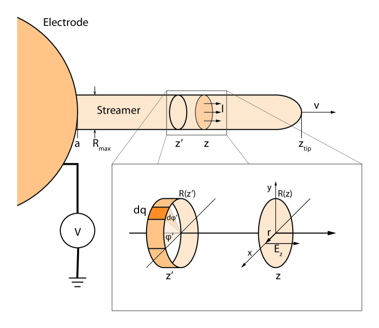
Figure 1: Schematic picture of our streamer model. We simulate a streamer that emerges from spherical electrode at a prescribed electrostatic potential $V$. The electrode has a radius $a$ and is centered at the origin. The streamer advances with velocity $v$ in the $z$-direction and its tip is located at the time-dependent position $z_{\text{tip}}$. Far to the left of the tip, the streamer channel assymptotocally approaches a maximum radius $R_{\text{max}}$. The inset shows the geometry the of electrostatic interaction whereby a charge element $\operatorname{d\!}q$ at $z^{\prime}$ contributes to the electric field at $z$ and thus to the electric current $I$ at that point.

Figure 1 shows a schematic view of our model. Although our approach can be generalized to other contexts, we focus on streamers in air at atmospheric pressure. We model the streamer as an axially symmetrical filament that grows in the $z$ direction due to the electric field created by a spherical electrode to which it is connected. At a given time $t$ the streamer spans the distance from the electrode boundary $a$ to the location of the streamer tip $z_{\text{tip}}$ and propagates at a velocity

$$v=\dfrac{\operatorname{d\!}{}z_{\text{tip}}}{\operatorname{d\!}{t}}.$$ (1)

The streamer shape is defined by its radius $R(z)$ in the range $a<z<z_{\text{tip}}$. In the simplest case we prescribe $R(z)$ to have a smooth shape around $z_{\text{tip}}$ and asymptotically approach a prescribed function $R^{\star}(z)$ far from the tip. A simple expression with these properties is

$$R(z)=R^{\star}(z)\left(1-e^{(z-z_{\text{tip}})/R^{\star}(z)}\right)^{1/2}.$$ (2)

At the streamer tip this shape yields a radius of curvature $R^{\star}(z_{\text{tip}})/2$ so $R^{\star}(z)$ encapsulates the evolution of the streamer radius. As mentioned in ref. [16], finding a physically motivated evolution for the streamer radius remains an unsolved problem of streamer physics. Here we will mostly impose a constant $R^{\star}(z)=R_{\text{max}}$, with the exception of section 4 where, to properly compare with a microscopic simulation, we impose that the radius grows at a constant rate in space, $R^{\star}(z)=R_{0}+Kz$, where $K$ is obtained from the microscopic simulation.

Our key assumption is that the streamer is so thin that we can consider that charge transport in the transversal direction occurs instantaneously. In that case all the electric charge accumulates at the streamer’s boundaries. This behaviour is observed in all microscopic streamer simulations (e.g. refs. [17, 18, 19, 20, 21, 22]). Under this assumption the full electrodynamic state of the streamer can be described by a linear charge density $\lambda$ that satisfies

$$\dfrac{\partial{}\lambda}{\partial{t}}=-\dfrac{\partial{}I}{\partial{z}},$$ (3)

where $I$ is the electric current flowing through the streamer cross section. As we discuss below, the current $I$ must include not only the volume current flowing through the streamer body but also a surface current located at the streamer boundary. We call these two components, respectively, channel current, $I_{C}$, and surface current, $I_{S}$.

2.1.1 The channel current.

This current is related to the electric current density $\mathbf{j}$ by an integral over the channel’s cross-section:

$$I_{C}=\int_{0}^{R(z)}j_{z}\,2\pi r\operatorname{d\!}r.$$ (4)

The current density $\mathbf{j}$ results from drift and diffusion of all charged species $s$ within the streamer:

$$\mathbf{j}=\sum_{s}\left(|q_{s}|\mu_{s}n_{s}\mathbf{E}-\nabla\cdot D_{s}n_{s}\right),$$ (5)

where $\mathbf{E}$ is the local electric field and $q_{s}$, $\mu_{s}$, $n_{s}$ and $D_{s}$ are respectively the charge, mobility, density and diffusion coefficient of species $s$.

To obtain a model that can be simulated efficiently and is expected to scale to multi-streamer simulations, we introduced a number of simplications. First, we neglect diffusion Also, as the inner electric field within a streamer does not exhibit too large a variability, almost always ranging from $3\text{\,}\mathrm{k}\mathrm{V}\mathrm{/}\mathrm{c}\mathrm{m}$ to $30\text{\,}\mathrm{k}\mathrm{V}\mathrm{/}\mathrm{c}\mathrm{m}$, we approximate the mobility of all species $\mu_{s}$ to be independent of the electric field. This assumption turns (3) into a linear differential equation, heavily simplifying its solution. A final simplification that we take for the sake of computing efficiency is that the species densities $n_{s}$ are uniform across the channel and can be taken out of the integral (4). Below we show that this yields a closed-form expression for one integral in a multi-dimensional integral expression, saving us one numerical integration.

With these simplifications (4) reads

$$I_{C}(z)=\sigma(z)\int_{0}^{R(z)}E_{z}(z,r)\,2\pi r\operatorname{d\!}r,$$ (6)

where

$$\sigma(z)=\sum_{s}q_{s}\mu_{s}n_{s}(z)$$ (7)

is the channel conductivity.

We calculate the electric field in (6) by decomposing it as $E_{z}=E_{0z}+E_{1z}$, where $E_{0}$ is the background field and $E_{1}$ is the self-consistent field created by the charges in the channel. The linearity of (6) translates this decomposition into a current $I_{C0}$ driven by the external field and a current $I_{C1}$ due to interactions between channel elements.

For the moment, we leave aside the current driven by the external field, $I_{C0}$, which we more conveniently discuss in section 2.1.3, after we have also discussed the surface current in 2.1.2.

Focusing on the channel current $I_{C1}$, which depends on the self-consistent field $E_{1}$, we consider the geometry in the inset of figure 1, where we are interested in the electric field at longitudinal coordinate $z$ and at distance $r$ away from the axis. To calculate this, we integrate the contributions of all charge elements $\operatorname{d\!}q$ at longitudinal coordinates $z^{\prime}$. The charge in $\operatorname{d\!}q$ is

$$\operatorname{d\!}q=\frac{1}{2\pi}\lambda\operatorname{d\!}\varphi^{\prime}\operatorname{d\!}z^{\prime},$$ (8)

where $\varphi^{\prime}$ is the azimuthal angle of the charge element. Let us first focus on electrostatic interactions in free space (i.e. in the absence of any electrode): the presence of an electrode is discussed in the following section. In free space the contribution of $\operatorname{d\!}q$ at $z^{\prime}$ to $E_{1z}$ at $z$ reads

$$\operatorname{d\!}E_{1z}=\frac{(z-z^{\prime})\operatorname{d\!}q}{4\pi\varepsilon_{0}\left[(r-R(z^{\prime})\cos\varphi^{\prime})^{2}+R(z^{\prime})^{2}\sin^{2}\varphi^{\prime}+(z-z^{\prime})^{2}\right]^{3/2}}.$$ (9)

In order to simplify our notation, it is convenient to introduce $x(z^{\prime},\varphi^{\prime})=R(z^{\prime})\cos\varphi^{\prime}$, $\rho(z^{\prime},\varphi^{\prime})=\left(R(z^{\prime})^{2}\sin^{2}\varphi^{\prime}+(z-z^{\prime})^{2}\right)^{1/2}$. For brevity we leave the dependence on $z^{\prime}$ and $\varphi^{\prime}$ implicit and write simply $x$ and $\rho$. With this notation and combining (8) and (9) into (6) we obtain

$$I_{C1}(z)=\frac{\sigma(z)}{4\pi\varepsilon_{0}}\int_{0}^{R(z)}\operatorname{d\!}r\int_{z_{b}}^{z_{\text{tip}}}\operatorname{d\!}z^{\prime}\int_{0}^{2\pi}\operatorname{d\!}\varphi^{\prime}\frac{(z-z^{\prime})\lambda(z^{\prime})r}{\left[(r-x)^{2}+\rho^{2}\right]^{3/2}}.$$ (10)

As we mentioned above, one of the three integrals in (10) can be solved analytically into a closed-form expression. For this we make use of the indefinite integral

$$\int\frac{r\operatorname{d\!}r}{\left[(r-x)^{2}+\rho^{2}\right]^{3/2}}=\frac{x(r-x)-\rho^{2}}{\rho^{2}\sqrt{\rho^{2}+(r-x)^{2}}}+C$$ (11)

and rewrite (10) as

$$I_{C1}(z)=\left.\frac{\sigma(z)}{4\pi\varepsilon_{0}}\int_{z_{b}}^{z_{\text{tip}}}\operatorname{d\!}z^{\prime}(z-z^{\prime})\lambda(z^{\prime})\int_{0}^{2\pi}\operatorname{d\!}\varphi^{\prime}\frac{x(r-x)-\rho^{2}}{\rho^{2}\sqrt{\rho^{2}+(r-x)^{2}}}\right|_{r=0}^{r=R(z)}.$$ (12)

Thus, defining a kernel

$$G_{C}(z,z^{\prime})=(z-z^{\prime})\int_{0}^{2\pi}\operatorname{d\!}\varphi^{\prime}\left.\frac{x(r-x)-\rho^{2}}{\rho^{2}\sqrt{\rho^{2}+(r-x)^{2}}}\right|_{r=0}^{r=R(z)},$$ (13)

we write (12) as

$$I_{C1}(z)=\frac{\sigma(z)}{4\pi\varepsilon_{0}}\int_{z_{b}}^{z_{\text{tip}}}\operatorname{d\!}z^{\prime}G_{C}(z,z^{\prime})\lambda(z^{\prime}).$$ (14)

Some comments about this electrodyamic model are in order:

1. The integrand in (12) diverges as $z^{\prime}\to z$ and $\varphi^{\prime}\to 0$. This of course stems from the divergence of the electric field around a point charge. However, one can prove that this divergence is integrable and the expressions (12) and (14) are well defined. Here we are calculating the field close to a surface with a smooth charge density, which is finite and well defined.

2. Microscopical simulations of streamers show that the electric field inside the streamer channel is transversally quite homogeneous. One is therefore tempted to skip the integrals in $r$ and $\varphi^{\prime}$ and take the electric field at the central axis as a good approximation. This approach, called ring method was employed e.g. by ref. [24] and is equivalent to replacing $G_{C}(z,z^{\prime})$ in (14) by

   $$G_{R}(z,z^{\prime})=\frac{\pi R(z)^{2}(z-z^{\prime})}{\left[R(z^{\prime})^{2}+(z-z^{\prime})^{2}\right]^{3/2}}.$$ (15)

   However, as mentioned in ref. [1], this approximation often leads to unrealistic oscillations in the presence of strong longitudinal inhomogeneities such as the streamer head itself. A comparison between $G_{C}(z,z^{\prime})$ and $G_{R}(z,z^{\prime})$, as shown in figure 2a, hints at an explanation. In the figure, where we have set $R(z)=1$ so that $G_{C}$ and $G_{R}$ become functions only of $z^{\prime}-z$, we see that the kernel $G_{R}$ vanishes as $z^{\prime}\to z$, which means that it neglects interactions between closely spaced rings in the streamer channel. As pictured in figure 2b, these interactions are dominated by the electric field away from the central axis; only when $z^{\prime}-z\gg R$ can we take (figure 2c) the electric field in the axis as representative of the full cross-sectional interaction.

   Our kernel $G_{C}$, defined by (13), is discontinuous and correctly accounts for interactions between neighboring points. This is necesary to dynamically remove unphysical oscillations with wavelengths of the order of the streamer radius $R$.

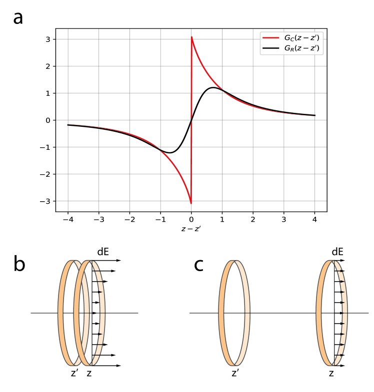
Figure 2: (a) Interaction kernels $G_{C}$ and $G_{R}$ defined by (13) and (15) in the text, plotted here for $R(z)=1$. (b) The short-range interaction in the streamer channel is dominated by electric fields and conduction currents off-axis; the ring kernel $G_{R}$ underestimates this interaction. (c) When the two annular sections are far appart the interaction field is transversally homogeneous and both kernels $G_{C}$ and $G_{R}$ give similar results.

2.1.2 The surface current.

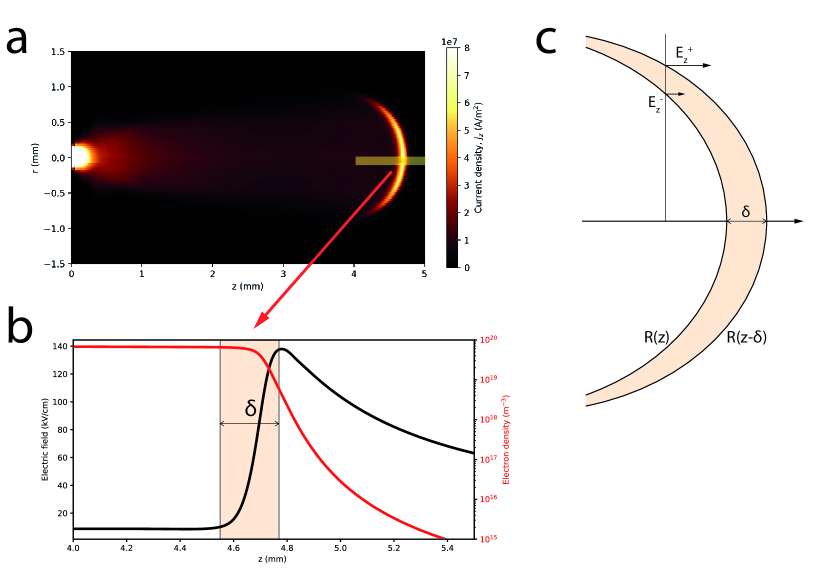
Figure 3: (a) A microscopic streamer simulation shows that close to the streamer tip there is a layer of electric current concentrated in a thin layer at the boundary. Details for this microscopic simulation are provided in section 4. (b) Profiles of the electric field and electron density on the central axis in the microscopic simulation. The approximate width of the current sheet ($\delta$) is indicated by the shaded region. (c) Scheme for the integration scheme of the current sheet used in our macroscopic model.

Besides the channel current described above, a streamer also contains a sheet of current around its head. This current, which we name here surface current, is apparent in figure 3a, where we show the electric current density obtained in a microscopic streamer simulation. The surface current is the main responsible of moving the space charge layer forward and it results from the continuous growth of the streamer channel. Figure 3b provides a microscopical interpretation of the suface current: the electric field is not fully screened close to the streamer head but rather penetrates a width $\delta$. Within this distance the electron density is already much higher that in the background so the penetration of the electric field results in a significant current.

To incorporate the surface current in our one-dimensional model we need first to estimate the width $\delta$ and then, in order to integrate across the channel, introduce reasonable assumptions about the electric field and electron density within the layer.

To estimate $\delta$ we note that the penetration of the field is a consequence of the finite conductivity of the channel combined with the streamer velocity. If we assume that within the streamer the field follows a dielectric relaxation with a characteristic time $\tau=\epsilon_{0}/\sigma(z_{\text{tip}})$, the width of the current layer is $\delta=\xi v\tau$, where $v$ is the streamer velocity and $\xi$ is a parameter of order unity that corrects for the curvature of the streamer head and the fact that the conductivity is not constant along the layer’s width. In our microscopic tests we found $\xi\approx 4$.

Figure 3c illustrates the transversal integration of the surface current at a given $z$. We approximate the channel conductivity ($\sigma$) and the $z$-component of the electric field ($E_{z}$) as linear functions between the inner and outer radius of the layer, respectively $R^{-}$ and $R^{+}$:

$$E_{z}(r)=E_{z}^{-}-\frac{(E_{z}^{-}-E_{z}^{+})(r-R^{-})}{R^{+}-R^{-}},$$ (16)

$$\sigma(r)=\sigma^{-}\frac{R^{+}-r}{R^{+}-R^{-}},$$ (17)

where $E^{-}$ and $E^{+}$ are the inner and outer values of the $z$-component of the electric field and where $\sigma^{-}$ is the inner conductivity, the outer conductivity being neglected.

We can apply (16) and (17) to integrate the electric current density $j_{z}=\sigma E_{z}$ across the channel width:

$$I_{S}=2\pi\int_{R^{-}}^{R^{+}}E_{z}(r)\sigma(r)r\,\operatorname{d\!}r=\frac{\pi}{6}\sigma^{-}(R^{+}-R^{-})\left[E^{+}(R^{+}-R^{-})+E^{-}(3R^{-}+R^{+})\right].$$ (18)

We incorporate (18) into our model by setting $R^{-}=R(z)$, $R^{+}=R(z-\delta)$, $\sigma^{-}=\sigma(z)$ and using (9) evaluated at $r=R(z)-\epsilon$ for $E^{-}$ and $r=R(z)+\epsilon$ for $E^{+}$, where $\epsilon$ is a small length that captures the discontinuity in the electric field at both sides of the thin charged layer . We take $\epsilon=$10\text{\,}\mathrm{\SIUnitSymbolMicro}\mathrm{m}$$.

Finally, we cast expression (18) into the same form as (14) by noting that (18) is linear in $E^{+}$ and $E^{-}$. We find

$$I_{S}(z)=\frac{\sigma(z)}{4\pi\varepsilon_{0}}\int_{z_{b}}^{z_{\text{tip}}}\operatorname{d\!}z^{\prime}G_{S}(z,z^{\prime})\lambda(z^{\prime}).$$ (19)

where

$$G_{S}(z,z^{\prime})=\frac{\pi}{6}(R^{+}-R^{-})\left[U^{+}(z,z^{\prime})(R^{+}-R^{-})+U^{-}(z,z^{\prime})(3R^{-}+R^{+})\right],$$ (20)

$$U^{\pm}(z,z^{\prime})=(z-z^{\prime})\int_{0}^{2\pi}\operatorname{d\!}\varphi^{\prime}\frac{1}{2\pi\left[(R(z)\pm\epsilon-x)^{2}+\rho^{2}\right]^{3/2}}.$$ (21)

Combining expressions (14) and (19) we calculate the total self-consistent current from a single kernel $G(z,z^{\prime})=G_{C}(z,z^{\prime})+G_{S}(z,z^{\prime})$:

$$I_{C1}+I_{S}=\frac{\sigma(z)}{4\pi\varepsilon_{0}}\int_{z_{b}}^{z_{\text{tip}}}\operatorname{d\!}z^{\prime}G(z,z^{\prime})\lambda(z^{\prime}).$$ (22)

2.1.3 Background field and inclusion of an electrode.

In most experiments, streamers start from an enhanced electric field around a high-voltage, pointed electrode. To reproduce this setup we consider here that the streamer emerges from a spherical electrode at an electrostatic potential $V$ (see figure 1) that is centered at the origin and has a radius $a$. In our model, we account for this electrode in two places: (a) in the background electric field $E_{0}$ introduced earlier and (b) in a modification of the kernel in (22) to include the effect of mirror charges required to satisfy the boundary conditions imposed by the electrode.

For the first point (a), the component of the total current due to the background field is what we called $I_{C0}$ in section 2.1.1. It can be calculated by integrating the $z$-component of the electric field created by the electrode, which yields

$$I_{C0}(z)=2\pi\sigma(z)aV\left(1-\frac{z}{\left(R(z)^{2}+z^{2}\right)^{1/2}}\right).$$ (23)

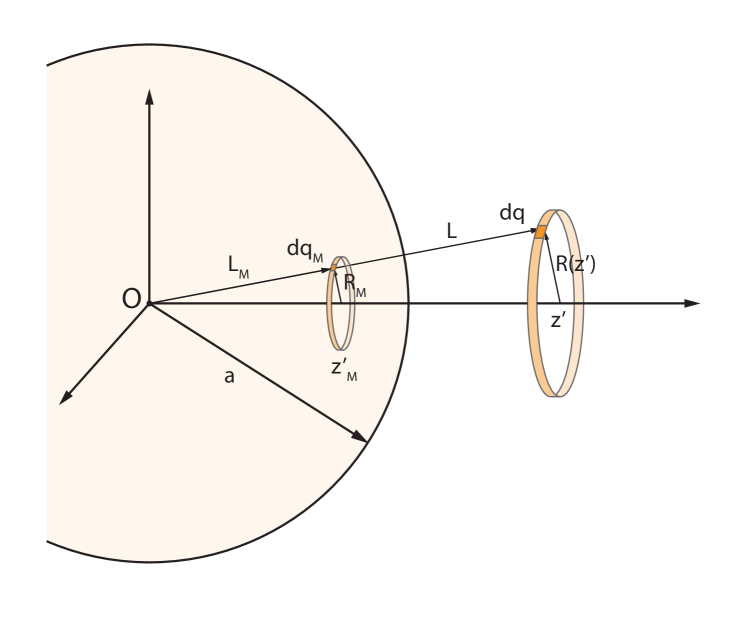
Figure 4: Computation of mirror charges required to satisfy the boundary conditions of an electrode of radius $a$. Here we consider a charge element $\operatorname{d\!}q$ at $z^{\prime}$, where the channel radius is $R(z^{\prime})$. The boundary condition imposed by the presence of a spherical electrode located at the origin are satisfied by including a mirror charge $\operatorname{d\!}q_{M}$ as described in the text.

Turning now to (b), in order to calculate the effect of mirror charges we consider the geometry shown in figure 4, where a charge element $\operatorname{d\!}q$ sits at axial coordinate $z^{\prime}$ and radius $R(z^{\prime})$. The boundary condition imposed by the presence of the electrode is satisfied if we include a mirror charge $\operatorname{d\!}q_{M}$ located on the line that joins the electrode’s center and $\operatorname{d\!}q$ and at a distance $L_{M}$. Following e.g. ref. [25] we find that $\operatorname{d\!}q_{M}=-\kappa\operatorname{d\!}q$, $L_{M}=\kappa^{2}L$, where $L=\left(z^{\prime 2}+R(z^{\prime})^{2}\right)^{1/2}$ and $\kappa=a/L$. The $z$-coordinate of $\operatorname{d\!}q_{M}$ is thus $z^{\prime}_{M}=\kappa^{2}z^{\prime}$. Therefore we include the effect of the electrode if we update the kernel function $G$ in (22) as

$$\bar{G}(z,z^{\prime})=G(z,z^{\prime};R(z^{\prime}))-\kappa G(z,\kappa^{2}z^{\prime};\kappa^{2}R(z^{\prime})),$$ (24)

where we made the dependence on $R(z^{\prime})$ explicit. Henceforth we calculate the self consistent current using $\bar{G}$ instead of $G$ in equation (22).

2.2 Chemical processes and mobilities

In general, many chemical reactions between active species operate within the streamer channel. These reactions influence the channel conductivity and must therefore be coupled to the electrodynamic evolution described in the previous section. Here we considered a chemical model composed of 17 species coupled through 78 reactions detailed in the supplementary material. The chemical model focuses on the evolution of electron density and ionic species following references [26, 27, 28] and includes the effect of water vapor as modeled by Gallimberti [29]. Note that this chemical model is designed to investigate changes in the conductivity for longer timescales than those considered in this work and thus many of the included reaction play a negligible role. Nevertheless we opted for keeping them as a reference.

The chemical model determines the evolution of the density of each species $s$ as

$$\dfrac{\partial{}n_{s}}{\partial{t}}=C_{s}=\sum_{r\in\text{reactions}}A_{sr}k_{r}n_{\mathcal{I}(r,1)}n_{\mathcal{I}(r,2)}\dots,$$ (25)

where $C_{s}$ is the net creation of species $s$, $A_{sr}$ is the net number of molecules of species $s$ created each time that reaction $r$ takes place, $k_{r}$ is the rate coefficient of reaction $r$ and $\mathcal{I}(r,1),\mathcal{I}(r,2),\dots$ are the indices of the input species of reaction $r$. Here the rate coefficient $k_{r}$ is, in general, a function of the local electric field. Since the transversal variation of the electric field is dynamically suppresed by the kernel described in the previous section, here it is justified to calculate the rate coefficients from the electric field at the streamer axis. Thus $k_{r}$ depends on

$$E_{\text{axis}}(z)=\frac{1}{4\pi\varepsilon_{0}}\int_{z_{b}}^{z_{\text{tip}}}\operatorname{d\!}z^{\prime}\bar{G}_{R}(z,z^{\prime})\lambda(z^{\prime}),$$ (26)

where $\bar{G}_{R}(z,z^{\prime})$ is the kernel function obtained from (15) by adding the effect of mirror charges as in (24).

As the streamer propagates (see next section), it changes the composition of the gas ahead of its tip through photo-ionization and the enhancement of the electric field. Our model does not include the dynamics ahead of the streamer tip so the effect of these processes is modeleled by imposing densities $n_{s}^{0}$ for each species $s$ at the streamer tip $z_{\text{tip}}$. We consider that the pre-streamer dynamics elevate the electron density to a prescribed value $n_{e}^{0}$; to ensure quasi-neutrality this density is balanced by concentrations of O2+ and N2+ that follow the relative densities of O2 and N2 in air. The densities of all other species are set to zero at $z_{\text{tip}}$.

All charged species contribute to the channel conductivity, which we calculate with (7). We take the electron mobility as $\mu_{e}=$380\text{\,}\mathrm{c}\mathrm{m}^{2}\mathrm{/}\mathrm{V}\mathrm{/}\mathrm{m}$$ [30]. For O-, O2- and O3- we use values from ref. [31] fetched from the LxCat database [32] selecting the approximate mobilities for a reduced electric field of $100\text{\,}\mathrm{T}\mathrm{d}$. This gives us

$$\mu =$4.5\text{\,}\mathrm{c}\mathrm{m}^{2}\mathrm{/}\mathrm{V}\mathrm{/}\mathrm{m}$,$$

$$\mu_{\cee{O2-}} =$2.7\text{\,}\mathrm{c}\mathrm{m}^{2}\mathrm{/}\mathrm{V}\mathrm{/}\mathrm{m}$,$$

$$\mu_{\cee{O3-}} =$2.8\text{\,}\mathrm{c}\mathrm{m}^{2}\mathrm{/}\mathrm{V}\mathrm{/}\mathrm{m}$.$$ (27)

Within our model’s accuracy, all other ions, including water cluster ions [33], can be assumed to have roughly the same mobility, which we take as

$$\mu_{\text{ion}}=$2\text{\,}\mathrm{c}\mathrm{m}^{2}\mathrm{/}\mathrm{V}\mathrm{/}\mathrm{m}$.$$ (28)

2.3 Streamer propagation

At the same time that charge is transported and chemical reactions are operating within the streamer channel, the streamer tip advances. It is generally accepted that the speed of this advance, as defined in (1), depends on the streamer’s radius and the electric field at its tip, $E_{\text{tip}}$. This is,

$$\dfrac{\operatorname{d\!}{}z_{\text{tip}}}{\operatorname{d\!}{t}}=v(E_{\text{tip}},R_{\text{max}}).$$ (29)

Here $E_{\text{tip}}$ can be evaluated from (26) as $E_{\text{tip}}=E_{\text{axis}}(z_{\text{tip}}^{+})$, where $z_{\text{tip}}^{+}$ means that, since the field is discontinuous at $z_{\text{tip}}$, we take the value immediately outside the streamer.

Naidis [34] investigated the relation between streamer radius, peak electric field and velocity. He considered the active area ahead of the streamer where the electric field is above the breakdown threshold $E_{p}$. By assuming that the multiplication factor $M$ of the electron density within this area (or rather, its logarithm) is roughly the same for all streamers, Naidis derived the following expression for the streamer velocity $v$:

$$\gamma R_{\text{max}}E_{\text{tip}}\int_{E_{p}}^{E_{\text{tip}}}\frac{\operatorname{d\!}E\,\nu(E)}{E^{2}(v\pm\mu_{e}E)}=\log M+\log\left(\frac{v\pm\mu_{e}E_{\text{tip}}}{v\pm\mu_{e}E_{p}}\right),$$ (30)

where $\gamma$ is a factor of order unity that relates the spatial decay of the electric field to the streamer radius (we assume $\gamma=1/2$), $\nu(E)$ is the field-dependent temporal growth rate of electrons and $\mu_{e}$ is their mobility. As proposed by Naidis, we take $\log M=8$.

The streamer velocity in our model is obtained by solving for $v$ in (30), given $R_{\text{max}}$ and $E_{\text{tip}}$. Nevertheless, in section 5 below, we investigate the effect of the velocity on a streamer’s properties by manually tuning the velocity for a given peak field and radius. With that purpose, we multiply the velocity $v$ resulting from (30) by a factor $\beta$.

3 Numerical implementation

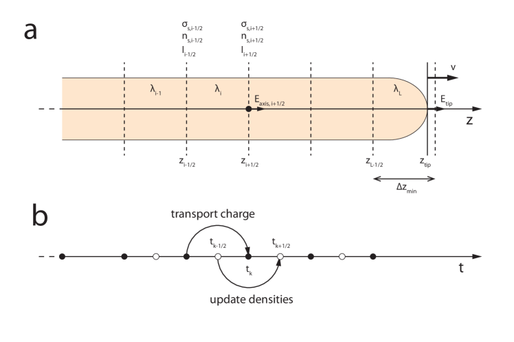
Figure 5: Spatial (a) and temporal (b) discretization schemes for solving our model. As described in the text, we implemented a finite volumes method where the streamer lenght is divided into $L$ cells, with average charge densities defined for each cell. At the cell boundaries we evaluate electric currents, species densities and conductivities. The time integration uses a leapfrog scheme that alternates between solving charge transport and updating densities and conductivities.

Figure 5 sketches the spatial and temporal discretizations that we implemented for the model described above. At a given time the streamer length is divided into cells $\mathcal{C}_{1},\mathcal{C}_{2},\dots\mathcal{C}_{L}$ with boundaries defined as $\mathcal{C}_{i}=(z_{i-1/2},z_{i+1/2})\dots\mathcal{C}_{L}=(z_{L-1/2},z_{\text{tip}})$. Note that the right boundary of the rightmost cell is $z_{\text{tip}}$ and that this boundary moves as the streamer advances. The rest of the cell boundaries are fixed within a time step but, as described below, the mesh structure is updated at certain times during the simulation.

To each cell we assign an average charge density $\lambda_{i}$ whereas the density of species $s$, $n_{s,i\pm 1/2}$, and the channel conductivity, $\sigma_{i\pm 1/2}$, are defined at the cell boundaries $z_{i\pm 1/2}$. We integrate in time using a leapfrog method, whereby we alternate between a step that advances the streamer head and solves (3) for charge tansport from time $t_{j-1}$ to $t_{j}$ and a step that solves the chemical system (25) from time $t_{j-1/2}$ to $t_{j+1/2}$. Let us describe each of these types of steps.

3.1 Charge transport and streamer progression

In the first kind of step, we integrate the transport of charge and advance the streamer tip from $t_{j-1}$ to $t_{j}$ assuming fixed particle densities and channel conductivity. To simulate the transport of charge through the streamer channel we implement a first-order accurate spatial discretization of (3). As the length of the rightmost cell of the streamer ($z_{\text{tip}}-z_{L-1/2}$), changes as the tip advances, our approach is more clearly formulated in terms of the total charge in a cell, $q_{i}=\lambda_{i}(z_{i+1/2}-z_{i-1/2})$. In these terms, the spatially discrete form of (3) reads

$$\dfrac{\operatorname{d\!}{}q_{i}}{\operatorname{d\!}{t}}=I_{i-1/2}-I_{i+1/2}.$$ (31)

In a charge-transport timestep, we integrate (31) calculating $I_{i\pm 1/2}$ from equations (22) and (23). For the self-consistent current we compute numerically the integrals involved in (22) using a Gauss-Legendre quadrature for $z^{\prime}$ within each cell and for the azimuthal angle $\varphi^{\prime}$. In our first-order accurate scheme we assume a constant linear charge density inside each cell, which leads to a linear system

$$I_{i+1/2}=\sum_{k=1}^{L}a_{ik}(t)q_{k}+b_{i}(t),$$ (32)

where the first term results from self-interaction ($I_{C1}+I_{S}$) and the second term from the background field ($I_{C0}$). Even though we fix conductivities $a_{ik}$ and $b_{i}$ change during a timestep due to the advancing streamer tip. Defining the matrix $\mathbf{W}(t)$ with elements $W_{ij}(t)=a_{i-1\,k}(t)-a_{ik}(t)$ and the vector $V(t)$ with components $V_{i}(t)=b_{i-1}(t)-b_{i}(t)$, (31) has the matrix form

$$\dfrac{\operatorname{d\!}{}q}{\operatorname{d\!}{t}}=\mathbf{W}(t)q+V(t).$$ (33)

This equation is coupled with equation (29), which determines the advance of $z_{\text{tip}}$. As this advance is generally smooth and not too far from uniform translation, an explicit Euler integration is accurate enough. Since the tip velocity depends on the peak electric field $E_{\text{tip}}$, we integrate (26) at $z=z_{\text{tip}}^{+}$ also by means of a Gauss-Legendre quadrature.

With this approach, given the status of the streamer at time $t_{j-1}$ we calculate $z_{\text{tip}}(t_{j})$ and thus $\mathbf{W}(t_{j})$ and $V(t_{j})$. We then integrate (33) in time with a semi-implicit Crank-Nicolson scheme, which yields the following linear system to obtain the charge at time $t_{j+1}$:

$$\left[\mathbf{1}-\frac{\Delta t}{2}\mathbf{W}(t_{j+1})\right]\mathbf{q}(t_{j+1})=\left[\mathbf{1}+\frac{\Delta t}{2}\mathbf{W}(t_{j})\right]\mathbf{q}(t_{j})+\frac{\Delta t}{2}\left[V(t_{j})+V(t_{j+1})\right].$$ (34)

3.2 Update of the species densities

Alternating with the step that we just described, we perform steps where, for given values of $\lambda_{i}$ and $z_{\text{tip}}$ at time $t_{j}$, we update the species densities and the channel conductivity from time $t_{j-1/2}$ to $t_{j+1/2}$. We integrate (26) with a Gauss-Legendre quadrature in each spatial cell to obtain $E_{\text{axis}}$ at points $z_{i\pm 1/2}$. From this we compute all chemical reaction rates $k_{r}$ in equation (25). Note that within this kind of timestep the temporal evolution of chemical species at a given point $z_{i\pm 1/2}$ is decoupled from all other points and can be solved independently. Here we also apply a Crank-Nicolson scheme but in this case this method leads to a nonlinear equation which we solve using the Newton-Raphson method.

3.3 Adaptation of the spatial mesh

So far we have described the update of streamer variables within a fixed spatial mesh (with the exception of the right boundary at $z_{\text{tip}}$). However, this scheme presents two problems:

1. The rightmost spatial cell, bounded by $z_{\text{tip}}$, grows disproportionally long. To prevent this, whenever the length of this cell exceeds a length $\Delta z$ we split it at $z_{L-1/2}+\Delta z$ and increase the total number of cells, $L$. We split the total charge in the cell assuming a constant charge density and we interpolate linearly the values of the species densities at the newly created cell boundary.

2. Generally we need a better resolution close to the streamer tip but it is wasteful to use similar cell sizes along the full length of the streamer. To improve the efficiency of the code without sacrificing too much accuracy we employ an adaptative mesh. Every $n_{\text{coarsen}}=10$ time steps we update our mesh by merging cells where an estimate of the logarithmic slope of the absolute value of the charge density is below a given threshold $\epsilon_{\text{coarsen}}=$5\text{\times}{10}^{-2}$$.

3.4 Implementation

Our simulations are dominated by the computation of electrostatic interactions. As we calculate all pairs of interactions between cells, it takes $O(L^{2})$ computations to find the time derivative of the charge density. Furthermore, each of these $O(L^{2})$ computations involves a two-dimensional integral (in $z^{\prime}$ and in $\varphi^{\prime}$). It is thus clear that computational efficiency was a prime concern for us.

Fortunately most of these calculations are independent from each other and therefore our problem is easily parallelizable. We developed two versions of our code: one runs in standard multicore processors and is parallelized using OpenMP and another is implemented using the Compute Unified Device Architecture (CUDA) and runs in General-Purpose Graphics Processing Units (GPGPUs). As the latter version benefits from massive parallelism it runs between 1.5 and 14 times faster than the OpenMP version, depending on the resolution.

In all simulations reported here we used time-steps $\Delta t=$2\text{\times}{10}^{-12}\text{\,}\mathrm{s}$$ and smallest spatial mesh size $\Delta z=$100\text{\,}\mathrm{\SIUnitSymbolMicro}\mathrm{m}$$.

4 Comparison with microscopic simulations

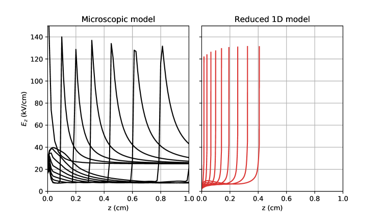
Figure 6: Comparison beween a microscopic streamer model (left) and the 1D model presented in this work (right). Both models are applied to a positive streamer propagating to the right under conditions as similar as possible given the differences between the two approaches. For each of the models we show the evolution of the axial electric field. All curves are plotted at regular intervals of $1\text{\,}\mathrm{n}\mathrm{s}$.

In this section we test the model described above and its implementation against a microscopic streamer code. For this purpose we use the existing ARCoS code, which has been previously applied to problems of streamer dynamics both at atmospheric pressure [35, 36] and in the context of high altitude atmospheric discharges (sprites) [37, 22, 38, 39]. The code is based on an adaptive-refinement scheme [19] and is capable of working with slightly non-axisymmetric streamers and inhomogeneous backgrounds (for a review see ref. [16]). The microscopic model implements a field-dependent electron mobility and includes electron impact ionization of N2 and O2 molecules as well as dissociative attachment to O2. Swarm parameters are solved offline using Bolsig+ [40] with the cross-sections from ref. [41] fetched from the LxCat database [32].

For our comparison we selected the propagation of a positive streamer at atmospheric pressure initiated from a needle mock-up as described in ref. [36] with a needle “lenght” of $2\text{\,}\mathrm{m}\mathrm{m}$ and a “radius” of $0.2\text{\,}\mathrm{m}\mathrm{m}$. We apply a potential difference of $50\text{\,}\mathrm{k}\mathrm{V}$ between this needle and a planar electrode located $2\text{\,}\mathrm{c}\mathrm{m}$ away from the tip. We start the streamer placing a neutral, spherical gaussian seed with an $e$-folding length of $0.15\text{\,}\mathrm{m}\mathrm{m}$ and a total of $4.6\text{\times}{10}^{9}$ free electrons.

Turning now to the parameters of the macroscopic, 1D model presented in this work, we simulate the protrusion-plane geometry of the microscopic model by starting from an existing $2\text{\,}\mathrm{m}\mathrm{m}$-long ionized channel attached to a conducting plane, which we simulate by using a large electrode radius in the geometry described in figure 1. To this configuration we apply an external uniform background electric field of $25\text{\,}\mathrm{k}\mathrm{V}\mathrm{/}\mathrm{c}\mathrm{m}$, which coincides with the average electric field in the microscopic simulation.

A major problem for this comparison is that in the microscopic model the streamer expands significantly. As mentioned above, lacking a self-consistent evolution of streamer radius is the main limitation of our 1D model. Nevertheless we can check if all other features of the model are consistent with the microscopic simulation by externally imposing a fixed dependence of the tip radius with respect to the streamer length. This was the motivation of introducing $R^{\star}(z)$ in (2). From the microscopic model and the configuration described above we found $R^{\star}(z)\approx R_{0}+Kz$ with $K=0.1$ and $R_{0}=$0.5\text{\,}\mathrm{m}\mathrm{m}$$.

The results of the comparison are plotted in figure 6, where we show the evolution of the axial electric field and the linear charge density. The figure shows that the 1D model underestimates the streamer velocity by about a factor 2. On the other hand, the peak electric field is very similar in both simulations.

For a given peak electric field and streamer radius the expression (30) provides an unequivocal value for the streamer velocity. Therefore we attribute the speed difference between the two models to (a) inaccuracies in how we model the radius evolution in the 1D model, in particular during the early stages of evolution and to (b) inaccuracies in expression (30), which are likely due to the strongly nonlinear nature of streamers and to the imprecise definition of radius in an actual or microscopically modelled streamer.

5 Results

As we mentioned in the introduction, one of the advantages of a simplified model such as the one we have introduced here is that we can manually adjust parameters that in microscopic simulations are emergent properties of the dynamics. This helps us to reason about the relationships between different streamer features.

In this section we take one set of reference parameters and investigate how the streamer dynamics are affected by changes in the most relevant of these parameters. The reference parameters are listed in table 1. With these parameters we run simulations for both positive and negative streamers, the only difference between the two being the signs in the velocity expression (30). Then we also run simulations where we altered one of the reference parameters. We show the outcome of these simulations for positive and negative streamers in figures 7 and 8.

Parameter	Description	Reference value
$a$	Radius of the electrode	$5\text{\,}\mathrm{m}\mathrm{m}$
$n_{e}^{0}$	Electron density at the streamer tip	$4\text{\times}{10}^{19}\text{\,}\mathrm{m}^{-3}$
$V$	Voltage of the electrode	$50\text{\,}\mathrm{k}\mathrm{V}$
$R_{\text{max}}$	Largest streamer radius	$1\text{\,}\mathrm{m}\mathrm{m}$
$\beta$	Extra factor to manually change the streamer velocity	1

Table 1: Main parameters for a streamer simulation in our 1D model and the values that we take as a reference to investigate their role.

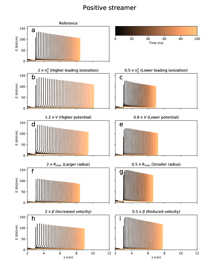
Figure 7: Effect of the most relevant parameters on the evolution of positive streamers. The uppermost plot shows the evolution of a streamer with the parameters of table 1; in each subsequent row we have altered one of these parameters. This change is denoted by, for example, $2\times\beta$, which indicates that in the corresponding simulation we increased $\beta$ by a factor 2. For each configuration we show snapshots of the axial electric field at intervals of $1\text{\,}\mathrm{n}\mathrm{s}$. Each snapshot is colored according to its time, as indexed in the colorbar at the top and right.

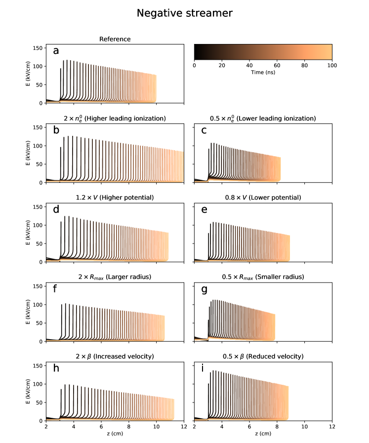
Figure 8: Effect of the most relevant parameters on the evolution of negative streamers. See the main text and the caption of figure 7 for a more complete description.

5.1 Differences between positive and negative streamers

The results in figures 7 and 8 show that our model is not yet predictive enough to explain some features commonly observed in streamer experiments and simulations. However, an examination of these features sheds some light on streamer physics and on the missing features of this model.

The first such feature that stands out is that in our case negative streamers propagate faster than positive streamers, something opposite to what is observed. This issue is discussed e.g. in ref. [36], where the higher velocity of positive streamers is attributed to a higher peak electric field, which in turns results from a sharper gradient of the electron density close to the head. Negative streamers, where electrons diverge from the head, have a more diffuse electron density and thus lower electric field and slower propagation.

Microscopic simulations show that the difference in propagation direction of electrons relative to the streamer translates into a higher electron density in the interior of positive streamers. Therefore to properly model differences between positive and negative streamers we have to not only change the signs in (30) but also our parameter $n_{e}^{0}$, which describes the multiplication of electrons ahead of the streamer.

5.2 Boundary electron density

As shown in figures 7 and 8, a change in $n_{e}^{0}$, which stands for the electron density at the streamer tip, has a significant effect on the properties of both positive and negative streamers. A higher leading ionization produces a stronger field enhancement and faster streamer propagation.

To simplify our discussion we assumed identical reference values of $n_{e}^{0}$ for positive and negative streamers but microscopic models clearly show that ionization is significantly stronger in positive streamers. An example can be found e.g. in ref. [42], where the difference is close to a factor 10. From this we conclude that although our model does not by itself explain the different velocities of streamers of opposite polarities, it can account for this difference by an appropriate selection of the parameter $n_{e}^{0}$.

5.3 Electrode potential

The effect of a change in the potential applied to the electrode is easier to explain. A higher potential leads to higher electric fields and faster propagation both in positive and negative streamers. The effect is stronger in positive streamers but this may be a consequence of our particular set of parameters.

5.4 Streamer radius

Focusing now on the effect of streamer radius, we see that in general a larger radius leads to a lower electric field but faster propagation. This is consistent with the observations of ref. [43], which were reproduced numerically in ref. [36]. The reason for this behaviour is that a larger radius implies a slower decay of the electric field ahead of the streamer, which greatly favours the multiplication of electrons and thus the further advance of the streamer. This is accounted for in the velocity expression (30) derived by Naidis, which, for a fixed peak electric field, predicts a higher velocity for a larger streamer radius.

But note that for a positive streamer, the velocity is almost unchanged between the reference simulation and the simulation with twice the streamer radius. In this case, the speed increase due to widening is compensated by the decrease due to a lower peak electric field. Here we also run into another limitation of our model: as a streamer evolves, its radius and peak electric field are interrelated. This means that in general in a real streamer a larger radius does not neccesarily imply a lower electric field. The experimental relationship between radius and velocity, which is better defined than in our simulations, may be explained if the peak field does not decrease substantially for wider streamers. This again underlines what we consider the main missing element in the model: a self-consistent evolution of streamer radius.

5.5 Velocity

As mentioned above, we multiplied the velocity resulting from expression (30) by a factor $\beta$ to investigate the role of streamer velocity. Unsurprinsingly, a larger $\beta$ leads to faster propagation.

However, in figures 7 and 8 we also see that artificially slowed-down streamers have a higher electric field at their tips. This illustrates the competing dynamics that take place in a streamer: the electrostatic relaxation of the streamer body strives to transport charge towards the tip but the ongoing propagation acts against this accumulation of charge. When we slow down the propagation we allow more charge to reach the streamer head where it creates a higher enhanced field. A quickly propagating streamer partly avoids this accumulation and therefore has a lower peak electric field.

6 Conclussions

The work presented here is a further step towards the objective of realistic and predictive simulations of complete discharge coronas. Although so far limited to single streamers, the model that we described includes a more accurate charge transport than the model of ref. [1]. Nevertheless, the discussion in the preceding section highlights some of the tradeoffs that we considered when designing our scheme:

1. The model includes parameters that have to be manually tuned in order to reproduce experimental observations. As we discussed above, to explain the differences between positive and negative streamers, we have to assume different values of $n_{e}^{0}$. Our model therefore has less predictive power than a microscopical simulation. We consider this an unavoidable price to pay for a macroscopic model. Similar limitations occur in almost all branches of Physics. For example, electromagnetic macroscopic models require material properties, such as electric permittivity, that must be obtained from microscopic calculations or directly from measurements.

2. A more troublesome limitation is the lack of a self-consistent evolution of the streamer radius. We have mentioned this issue at several places in this work and, as we discussed in section 4, an evolving streamer radius is neccesary to account for the streamer dynamics observed in microscopic simulations. We believe that this outstanding topic of streamer physics deserves to be the subject of future work.

Even with those limitations, the model that we presented can be extended to more realistic models of corona discharges that incorporate the strongly inhomogeneous field and electron density in the corona interior. In principle our scheme can be generalized to many interacting streamers with arbitrary shapes. To achive that, however, further numerical optimizations are required.

The final objective of this type of approach to streamer modeling is to couple it with the progression of a leader in order to understand how sections of the streamer corona are heated and join the leader channel. We hope that this article contributes to bring this objective somewhat closer.

Acknowledgments.- This work was supported by the European Research Council (ERC) under the European Union H2020 programme/ERC grant agreement 681257 and by the Spanish Ministry of Science and Innovation, MINECO under projects FIS2014-61774-EXP and ESP2015-69909-C5-2-R.

References

- [1] Luque A and Ebert U 2014 New Journal of Physics 16 013039 (Preprint 1307.2378)
- [2] Lozanskiĭ É D 1975 Soviet Physics Uspekhi 18 893
- [3] Kao C Y, Brau F, Ebert U, Schaefer L and Tanveer S 2010 Phys. D 239 1542–1559 ISSN 0167-2789
- [4] Arrayás M, Fontelos M A and Jiménez C 2010 Phys. Rev. E 81 035401 (Preprint 0910.3617)
- [5] Ebert U, Brau F, Derks G, Hundsdorfer W, Kao C Y, Li C, Luque A, Meulenbroek B, Nijdam S, Ratushnaya V, Schäfer L and Tanveer S 2011 Nonlinearity 24 1
- [6] Meulenbroek B, Rocco A and Ebert U 2004 Phys. Rev. E 69 067402 (Preprint physics/0305112)
- [7] Meulenbroek B, Ebert U and Schäfer L 2005 Phys. Rev. Lett. 95 195004 (Preprint nlin/0507019)
- [8] Arrayás M, Fontelos M A and Kindelán U 2012 Phys. Rev. E 86 066407 (Preprint 1203.6790)
- [9] Brau F, Luque A, Meulenbroek B, Ebert U and Schäfer L 2008 Phys. Rev. E 77 026219 (Preprint 0707.1402)
- [10] Brau F, Luque A, Davidovitch B and Ebert U 2009 Phys. Rev. E 79 066211 (Preprint 0901.1916)
- [11] Brau F, Davidovitch B and Ebert U 2008 Phys. Rev. E 78 056212
- [12] Arrayás M and Fontelos M A 2011 Phys. Rev. E 84 026404 (Preprint 1103.0404)
- [13] Niemeyer L, Pietronero L and Wiesmann H J 1984 Phys. Rev. Lett. 52 1033
- [14] Pasko V P, Inan U S and Bell T F 2000 Geophys. Res. Lett. 27 497
- [15] Akyuz M, Larsson A, Cooray V and Strandberg G 2003 J. Electrost. 59 115 – 141 ISSN 0304-3886
- [16] Luque A and Ebert U 2012 J. Comput. Phys. 231 904
- [17] Dhali S K and Williams P F 1985 Phys. Rev. A 31 1219
- [18] Pancheshnyi S V and Starikovskii A Y 2003 J. Phys. D 36 2683
- [19] Montijn C, Hundsdorfer W and Ebert U 2006 J. Comput. Phys. 219 801 (Preprint physics/0603070)
- [20] Luque A, Ebert U, Montijn C and Hundsdorfer W 2007 Appl. Phys. Lett. 90 081501 (Preprint physics/0609247)
- [21] Babaeva N Y and Kushner M J 2009 Plasma Sour. Sci. Technol. 18 035009
- [22] Luque A and Ebert U 2010 Geophys. Res. Lett. 37 L06806
- [23] Dujko S, Ebert U, White R D and Petrović Z L 2011 Japanese Journal of Applied Physics 50 08JC01
- [24] Aleksandrov N L and Bazelyan E M 1996 J. Phys. D 29 740
- [25] Jackson J 1975 Classical electrodynamics (New York, USA: John Wiley and sons) ISBN 9780471431329
- [26] Kossyi I A, Kostinsky A Y, Matveyev A A and Silakov V P 1992 Plasma Sour. Sci. Technol. 1 207
- [27] Aleksandrov N L and Bazelyan E M 1999 Plasma Sour. Sci. Technol. 8 285
- [28] Pancheshnyi S 2013 J. Phys. D 46 155201
- [29] Gallimberti I 1979 Journal de Physique 40 193
- [30] Dhali S K and Williams P F 1987 J. Appl. Phys. 62 4696
- [31] Viehland L A and Mason E A 1995 At. Data Nucl. Data Tables 60 37
- [32] Pancheshnyi S, Biagi S, Bordage M C, Hagelaar G J M, Morgan W L, Phelps A V and Pitchford L C 2012 Chem. Phys. 398 148
- [33] Wissdorf W, Seifert L, Derpmann V, Klee S, Vautz W and Benter T 2013 Journal of The American Society for Mass Spectrometry 24 632
- [34] Naidis G V 2009 Phys. Rev. E 79 057401
- [35] Luque A, Ebert U and Hundsdorfer W 2008 Phys. Rev. Lett. 101 075005 (Preprint 0712.2774)
- [36] Luque A, Ratushnaya V and Ebert U 2008 J. Phys. D 41 234005 (Preprint 0804.3539)
- [37] Luque A and Ebert U 2009 Nature Geoscience 2 757
- [38] Luque A and Gordillo-Vázquez F J 2011 Geophys. Res. Lett. 38 L04808
- [39] Luque A, Stenbaek-Nielsen H C, McHarg M G and Haaland R K 2016 J. Geophys. Res. (Space Phys) 121
- [40] Hagelaar G J M and Pitchford L C 2005 Plasma Sour. Sci. Technol. 14 722
- [41] Phelps A V and Pitchford L C 1985 Phys. Rev. A 31 2932
- [42] Ihaddadene M A and Celestin S 2015 Geophys. Res. Lett. 42 5644
- [43] Briels T M P, Kos J, Winands G J J, van Veldhuizen E M and Ebert U 2008 J. Phys. D 41 234004 (Preprint 0805.1376)